José Eduardo Boffino de Almeida Monteiro(1), Letícia da Costa Azevedo(2), Eduardo Delgado Assad(2) and Paulo Cesar Sentelhas(3)
(1)Embrapa Uva e Vinho, Caixa Postal 130, CEP 95700‑000 Bento Gonçalves, RS, Brazil. E‑mail: [email protected] (2)Embrapa Informática Agropecuária, Caixa Postal 6041, CEP 13083‑886 Campinas, SP, Brazil. E‑mail: [email protected], [email protected] (3)Universidade de São Paulo, Escola Superior de Agronomia Luiz de Queiroz, Departamento de Engenharia de Biossistemas, Caixa Postal 9, CEP 13418‑900 Piracicaba, SP, Brazil. E‑mail: [email protected]
Abstract – The objective of this work was to evaluate an estimation system for rice yield in Brazil, based on simple agrometeorological models and on the technological level of production systems. This estimation system incorporates the conceptual basis proposed by Doorenbos & Kassam for potential and attainable yields with empirical adjusts for maximum yield and crop sensitivity to water deficit, considering five categories of rice yield. Rice yield was estimated from 2000/2001 to 2007/2008, and compared to IBGE yield data. Regression analyses between model estimates and data from IBGE surveys resulted in significant coefficients of determination, with less dispersion in the South than in the North and Northeast regions of the country. Index of model efficiency (E1') ranged from 0.01 in the lower yield classes to 0.45 in higher ones, and mean absolute error ranged from 58 to 250 kg ha‑1, respectively.
Index terms: crop simulation model, crop yield forecast, model efficiency, water deficit.
Estimativa da produtividade de arroz baseada em condições meteorológicas
e no nível tecnológico dos sistemas de produção no Brasil
Resumo – O objetivo deste trabalho foi avaliar um sistema de estimativa de produtividade da cultura do arroz no Brasil, com base em modelos agrometeorológicos simples e no nível tecnológico dos sistemas produtivos. Este sistema de estimativa incorpora as bases conceituais propostas por Doorenbos & Kassam para produtividades potenciais e alcançáveis com ajustes empíricos para produtividade máxima e sensibilidade da cultura à deficiência hídrica, considerando-se cinco classes de produtividade de arroz. A produtividade de arroz foi estimada de 2000/2001 a 2007/2008 e comparada aos dados do IBGE. Análises de regressão entre as estimativas do modelo e dados do IBGE resultaram em coeficientes de determinação significativos, com menor dispersão na região Sul do que nas regiões Norte e Nordeste do país. O índice de eficiência do modelo (E1') variou de 0,01, nas classes de menor produtividade, a 0,45 nas classes de maior produtividade, e o erro médio absoluto variou de 58 a 250 kg ha‑1, respectivamente.
Termos para indexação: modelo de simulação de cultura, previsão de safra, eficiência do modelo, deficiência hídrica.
Introduction
Crop yield forecasting and the knowledge of yield distribution are extremely important for governmental planning. This information is essential for public policy formulation, logistic distribution, food security, and for price formation at national and international markets
(Figueiredo, 2005). Yield forecasting applications can be conducted either prior to crop planting or during the growing season. The main objective is to predict yield, since this information can be used at farm‑level for marketing decisions or at government level for policy
issues and food security decisions (Hoogenboom,
2000).
Information on Brazilian total production, cropped area and yield can be obtained from crop surveys conducted by Companhia Nacional de Abastecimento
(the national supply company, Conab) and Instituto Brasileiro de Geografia e Estatística (Brazilian Institute
of Geography and Statistics, IBGE). These surveys are done for each municipality through interviews with local farmers, agronomists and technicians of cooperatives,
agricultural offices and technical assistance agencies.
process for surveys and field data consolidation, which
undermines the use of this information during the growing season, either for public policy measures or for crop management by farmers and cooperatives.
Agrometeorological monitoring systems (AMS)
provide, in near real time, information on meteorological conditions in the production regions. This system, when associated to crop yield simulation models, allows to quantify the impacts of meteorological conditions on agricultural yield – also in near real time –, in different phases of crop development.
Rice is cultivated and consumed in all continents
and has a strategic status (Heinemann et al., 2009) in Brazil and in many other countries. However, it is
very sensitive to weather conditions, with high‑water
requirement per unit of produced mass. Water deficit,
even if moderate, can cause high‑yield losses,
especially when occurring during flowering and early grain filling (Heinemann & Stone, 2009). Therefore,
upland rice crops are considered under high climate
risk (Silva & Assad, 2001)
Many models have been developed for crop
yield estimation considering different parameters and complexity levels, most of them are based on
agrometeorological variables (Doorenbos & Kassam, 1979; Assad et al., 2007; Heinemann & Stone, 2009).
There is a group of simulation models for rice yield estimation and forecasting, among them is Infocrop
(Aggarwal et al., 2006), Warm (Confalonieri et al., 2009) and Oryza (Bouman et al., 2006). In Brazil, some
of these models have been parameterized, like Oryza/
Apsim for upland (Lorençoni et al., 2010) and irrigated
rice, which is based in temperature and solar radiation
(Klering et al., 2008). However, despite all those
advances in crop modeling, a challenge still needs to be addressed in Brazil. This challenge relies on integrating a reasonable yield model with the large amount of data provided annually by Conab and IBGE for the whole country. To accomplish this task, two major issues have to be overcome: the lack of information about crop, soil, and production systems for all the production regions; and the inaccuracy of crop surveys, which are done by sampling and not always produce exact results for all the municipalities. An additional constraint is the fact that the available statistics show only the total production per municipality, regardless of whether it comes from irrigated or rainfed rice. For this reason, to successfully estimate rice yield in all production
areas of Brazil, it is crucial that the estimation system somehow consider the different types of crop systems
and their sensitivity to water deficit.
The objective of this work was to evaluate an estimation system for rice yield in Brazil, based on simple agrometeorological models and on the technological level of production systems.
Materials and Methods
The crop yield simulation model developed in the present study follows the theoretical basis proposed
by Doorenbos & Kassan (1979), which establishes
relationships between relative yield losses and
relative water deficiency along the crop phases. It
was composed by two modules: one that estimates crop potential yield or maximum yield; and other that estimates the decrement of potential yield as a function
of water deficit.
The proposed model was calibrated with basis on rice yield data derived from production and harvested area series surveyed by IBGE, for the growing seasons from 2000/2001 to 2007/2008. From the total of
5,561 municipalities, only 3,840 with data for at least
four crop seasons during the evaluated period were
considered. Municipalities were classified into five
categories, according to the average yield in the last four seasons. Intervals of each yield class included areas of upland rice and irrigated rice, and were set as follows: class 1, from 0 to 2,000 kg ha‑1; class 2, from 2,001 to 4,000 kg ha‑1; class 3, from 4,001 to
6,000 kg ha‑1; class 4, from 6,001 to 8,000 kg ha‑1; and class 5, from 8,001 to 10,000 kg ha‑1. Each yield class was analyzed independently, in order to produce
specific parameterization for each of them in modules
of both maximum and actual yields.
Normal sowing periods were identified for each state, according to Conab’s annual surveys (Companhia
Nacional de Abastecimento, 2009). In order to represent the distribution of planted areas of a state across time,
a frequency distribution of planted area (FDPA) was
adjusted to the sowing period, i.e. from mid‑October to mid‑December, in the state of Goiás, with higher concentration in November. FDPA was set to match start date, end date, and date of maximum planting of the whole sowing period. A proportion of planted area in each day was determined, within planting period,
Maximum yield, named as technological maximum yield (TYm), was estimated from a statistical
adjustment based on data series of observed actual yield. Observed yields were assumed as those which actually occurred in each municipality, which are surveyed and
published by IBGE every year (Instituto Brasileiro de Geografia e Estatística, 2010). The first step consisted in adjusting a first degree linear equation (Y = ax + b) to the observed yield data (Ya) against time (year). The
straight line generated by the equation indicates the
observed yield trend over years (Ya'). Yield deviations
that may happen over and under the line are caused by variation in productivity factors, including weather conditions, water availability and crop management. The second step consisted in determining a correction factor that, when multiplied by the observed yield
trend (Ya'), would elevate values to the yield level
without water restriction. This correction factor was
named coefficient of technological maximum yield (Δp). Thus, technological maximum yield (TYm)
was calculated for each year “n” as a function of the
adjusted actual yield multiplied by Δp: TYm = Ya' × Δp. In this sense, Δp was adjusted through a detrended
regression, and consisted in one of the parameters calibrated in this model, according to the method shown ahead.
Values of crop coefficient (kc) and yield response factor (ky) – presented by Heinemann et al. (2009)
for initial vegetative development, late vegetative
development, flowering, and maturation phases of rice – were adapted to the daily scale. Crop coefficient (kc) values, in the present work, were 0.4, 0.9, 1.3,
and 1.0, respectively, whereas yield response factor
(ky) were 0.2, 0.6, 1.25, and 0.4. Daily weather
data were used from 1,053 weather stations, spread throughout the Brazilian states, to estimate potential evapotranspiration. These stations are owned by governmental and private institutions and integrate the
Embrapa’s Agrometeorological Monitoring System (Agritempo). Actual crop evapotranspiration (ETa) was
determined by sequential water balance, computing daily changes in soil water content, according to Thornthwaite´s method. Due to the impossibility of precisely inferring the water holding capacity most suited for soils of different municipalities, an effective depth of the root system of 35 cm was considered for upland rice, as well as the water holding capacity of 1 mm cm‑1 (Araújo & Assad, 2001).
Actual yield (Ya) was estimated from the relationship between relative water deficit [1 - (ETa/ETc)] and
relative crop yield loss, weighted by the yield
response factor to water deficit (ky), for each
phenological phase, resulting in the following
model, presented in Doorenbos & Kassam (1979), Ya/Ym = 1 - ky[1 - (ETa/ETc)], in which: Ym
is the maximum yield, ETa is the actual crop evapotranspiration, and ETc is the maximum crop evapotranspiration. One of the changes in this model, if compared to the one cited above, is that yield calculation is updated daily, whenever the system receives new weather data, at the end of each day, similarly to the
system developed for soybean by Assad et al. (2007) in
Brazil. Another difference is the introduced empirical
parameter, called adjusted yield response factor (ky*),
bellow explained, which results in higher or lower
response to water deficit, according to technological specificities related to different production systems,
in each yield class. The third and last difference is
the use of the technological maximum yield (TYm). With all these changes, the final model results in: Ya/TYm = 1 - ky* × ky[1 - (ETa/ETc)]. In this
equation, TYm is used as the initial reference to begin the calculation process in each season. Once Ya of
the first day is calculated, it will be used as the new
reference in replacement to TYm in the second day, and so on.
Parameterization process consisted in adjusting the
maximum yield coefficient (Δp) and the adjusted yield response factor (ky*), in order to maximize correlation
between estimated and observed actual yields, and
also to minimize mean absolute error (MAE) between them. In this process, ky* starts with value 1.0 and
is subsequently increased or decreased according to
the gain or loss in the correlation and in the MAE
between estimated and observed yields. References used for evaluating model estimations were the independent yield values, surveyed and published by
IBGE (Instituto Brasileiro de Geografia e Estatística,
2010). These data came from 143 municipalities with complete yield data series from 2001 to 2008, distributed in four yield classes, with weather stations
located in the same municipality. The fifth yield class,
balance. When data were missing, the crop season was disregarded. From the total of municipalities, 71 were used for model parameterization and 72 for model performance evaluation.
Estimated Ya values (P) were compared to those from IBGE (O) by regression analysis and also by evaluating absolute and relative errors. The significance of the coefficient of determination (R2) was determined by T
test at 5% and 1% of probability. Model accuracy was evaluated according to the Legates’ modified index of model efficiency (E1') (Legates & McCabe Junior, 1999), as given in the following equation:
in which: E1' is the ratio of the mean error to the variance in the observed data, subtracted from the unity; and O and P stands for observed and predicted Ya values,
respectively. Thus, a zero value for the coefficient of efficiency indicates that the observed mean is as good
a predictor as the model, negative values indicate that the observed mean is a better predictor than the model, and positive values indicate better predictions than the observed mean.
Results and Discussion
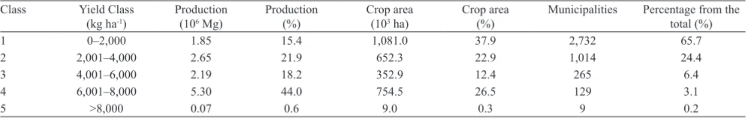
About 63% of the Brazilian rice production was
concentrated in 403 high‑yielding municipalities,
where flood irrigated systems are typical (Table 1).
Although the remaining 37% came from upland
rainfed rice, with lower yield, its fields were spread over 3,746 municipalities, which gives an idea of the
widespread cultivation of this crop in the country. The average yield of upland rice in Brazil is around 1,800 kg ha‑1, much lower than those observed for
flooded rice, which is about 6,110 kg ha‑1 (Instituto Rio Grandense do Arroz, 2008). Therefore, the production in municipalities of yield classes 1 and 2 is likely to be
from upland rice, while production in municipalities of classes 3 and 4 is likely to be predominantly from lowland irrigated crops. Upland rice naturally shows
lower maximum yield than flood–irrigated rice, which shows lower yields even without water deficits. Thus,
it is expected that lower the yield of a municipality, the higher is the proportion of rainfed crops. At this point, it is convenient to emphasize that this model is suited to estimate yield variability of rainfed crops. For irrigated rice, it is limited to the determination of yield trends, besides being a manner to distinguish irrigated from rainfed rice. This large distinction between yields of irrigated and rainfed rice allowed to minimize the effect of it in the estimations. Classifying municipalities by yield classes, with independent
calibration of ky* for each one, allowed to identify the degree of susceptibility to water deficits for each of them (Table 2).
The ky* and Δp calibration process was performed
in order to obtain the higher correlation and the smaller
absolute error possible. After calibration, ky* tended to zero with higher rice yields. A small ky* value indicates lower crop susceptibility to local water deficit. The Δp values reflected the average loss for each class during
the studied period, i.e. 30% in class 1 and 5% in class 4.
Coefficients of determination between estimated
and observed yields were high, even when the effect
of water deficiency was lower, and the inter-annual variations were smaller, as in class 3 and 4. However,
E1' was very low in classes of low productivity. In class 1, despite estimated yields represented well the
variations in IBGE series (R2 = 0.76), E
1' was very sensible to systematical error. For yield class 1, an error of 250 kg ha‑1 represents a high error of 25% relatively to the average yield, while the same absolute error represents a relative error of 3.8% in yield class 4.
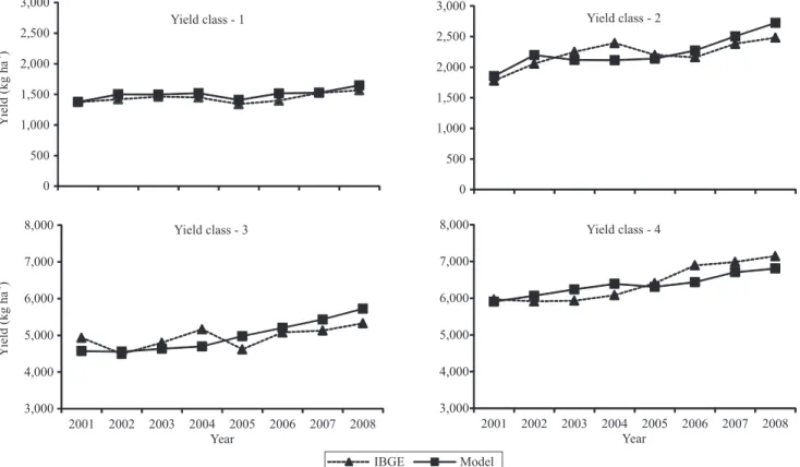
In general, yield model estimations were comparable to IBGE data trend over the years
(Figure 1). Some differences were observed in the
yield class 2 in 2004, and in the class 3, in 2004 and
Table 1. Rice production and number of producing municipalities per yield class, in 2008.
Class Yield Class
(kg ha‑1)
Production (106 Mg)
Production
(%) Crop area (103 ha)
Crop area
(%) Municipalities Percentage from the total (%)
1 0–2,000 1.85 15.4 1,081.0 37.9 2,732 65.7
2 2,001–4,000 2.65 21.9 652.3 22.9 1,014 24.4
3 4,001–6,000 2.19 18.2 352.9 12.4 265 6.4
4 6,001–8,000 5.30 44.0 754.5 26.5 129 3.1
2005. Classes 2 and 3 also showed the highest mean relative errors, possibly for being located in regions
where both systems (rainfed and irrigated) are used.
Different proportions of each crop system in a same municipality may result in over‑ or underestimation
of yield. Moreover, differences in water availability
and in crop management can also result in missing estimations of yield. This occurs because models are parameterized per yield class considering the data
set of the country as a whole, as there are no specific
parameterization per region.
Since systematic errors can be corrected through recalibration, the most important is quantifying the
inter-annual variability. Therefore, the coefficient of determination (R2) is a useful indicator. More attention should be given to cases where estimated yield shows one trend, and observed yield shows an opposite one. In these cases, the sources of error can be related to eventual changes in agricultural practices and management, which include used genotypes, soil management, fertilization, diseases and pests outbreaks etc. These are factors not computed by this model, due the impossibility of systematically survey them in the wide areas to be considered. Therefore, unpredictable variations may occur and degrade the model performance estimated by R2, MAE, MRE, and E1'.
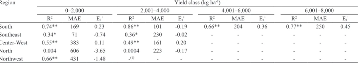
Lower R2 and E
1' were observed for regional‑scale
evaluations in most cases (Table 3). The lower model
performance in these evaluations shows that the parameterization with national data sets is not readily
available to be extrapolated to more specific areas.
Table 2. Technological maximum yield coefficient (Δp),
adjusted yield response factor to water deficit (ky*), mean absolute error (MAE), mean relative error (MRE), coefficient of determination (R2), and index of model efficiency (E
1’) between estimated and observed yields.
Class Yield class (kg ha‑1)
Δp ky* MAE
(kg ha‑1) MRE
(%) R
2 E
1’
1 0–2,000 1.30 2.4 58 4.1 0.76** 0.01
2 2,001–4,000 1.20 1.6 141 6.4 0.59** 0.12
3 4,001–6,000 1.11 0.6 204 4.3 0.66** 0.36
4 6,001–8,000 1.05 0.1 250 3.8 0.77** 0.45
5 >8,000 ‑(1) ‑ ‑ ‑ ‑ ‑
(1)Data not available.**Significant at 1% probability.
A potential limitation in this case might be the uneven distribution of municipalities in each region, since
yield class frequencies vary for each region. However,
South region had a better model performance than that of national data. In that region, the model simulated the occurrence of yield losses in 2005,
in classes 1 and 2 (Figure 2), due to an abnormally
intense drought in that year, mainly in the state of Rio Grande do Sul. Observed and estimated yields in class 4, however, were not reduced in 2005, due to the evident predominance of irrigated rice crops in that class. But, even in these classes, extreme droughts may affect water reservoirs and limit water availability for irrigation, which is a situation that could not be estimated. With these extreme events, observed yields should be reduced, while estimated yields would remain in the main trend. Data from the municipality of Pelotas in 2005 is a possible example
(Figure 3). Similar results were reported in Assad et al. (2007), when soybean showed high-yield losses
in 2005 in this region.
Yield estimations were made individually for each year and municipality, and for each year and yield class
(Figure 4). A clear difference was observed between the lower yield (0 to 2,000 and 2,000 to 4,000 kg ha‑1),
and the higher yield classes (4,000 to 6,000 and 6,000
to 8,000 kg ha‑1). Municipalities grouped into the classes 1 and 2 had average yields of 1,440 kg ha‑1 and 2,200 kg ha‑1, respectively. In contrast, municipalities of class 3 and 4 had average yields of nearly 5,000 kg ha‑1
and 6,300 kg ha‑1.
An important aspect to be addressed is the water availability in each phenological stage of the crop. The detailed approach, which weights the areas according to each sowing date, throughout the entire sowing period, is an attempt to reduce the main source of error regarding water availability. As the planting season may extend for up to 3.5 months, this may result in very different water conditions in areas planted at the beginning of the season or at the end of it. Due to the shallow root system of rice, even the nonirrigated crops explore small water reservoir
Table 3. Coefficient of determination (R2), mean absolute error (MAE), and index of model efficiency (E
1') between estimated and observed rice yield, per yield classes.
Region Yield class (kg ha‑1)
0–2,000 2,001–4,000 4,001–6,000 6,001–8,000
R2 MAE E
1' R2 MAE E1' R2 MAE E1' R2 MAE E1'
South 0.74** 169 0.23 0.86** 101 ‑0.19 0.66** 204 0.36 0.77** 250 0.45
Southeast 0.34* 71 ‑0.74 0.36* 230 ‑0.02 ‑ ‑ ‑ ‑ ‑ ‑
Center‑West 0.55** 383 0.11 0.49** 161 0.20 ‑ ‑ ‑ ‑ ‑ ‑
North 0.004 606 -3.65 0.0004 223 ‑0.17 ‑ ‑ ‑ ‑ ‑ ‑
Northwest 0.66** 431 ‑1.48 ‑(1) ‑ ‑ ‑ ‑ ‑ ‑ ‑ ‑
(1)Data not available.*and**Significant at 5 and 1% probability.
Figure 2. Observed and estimated rice yield in the Southern region of Brazil, for the growing seasons from 2001 to 2008,
in the soil, being hard to determine precisely the water holding capacity for each site or yield class. Therefore, small inaccuracies in estimating actual daily evapotranspiration, accumulated in a given
period (e.g. 10 days), should not exceed the water deficit accumulated in 2 or 3 days of water restriction,
in order to not compromise yield estimations.
Moreover, within a sowing period of more than three months, crops may reach critical stages (e.g.
flowering) under water conditions very different from
those observed in areas planted sooner or later. Given the gradual depletion of water in soil, the number of days of water stress becomes a more important factor in estimating yield than minor inaccuracies in the water balance calculation.
Despite the water factor, the use of technological maximum yield concept, with correction of yield trends over time, is important to improve accuracy and
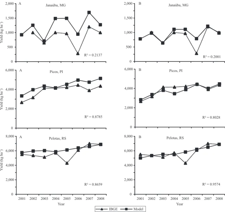
Figure 3. Rice yield variation estimated by the model, and observed rice yield (Instituto Brasileiro de Geografia e Estatística,
precision of estimates in both low and high yield classes. This reference yield represents the actual portion of the theoretical potential yield that can be achieved, depending on the available technology for inputs and crop management techniques. Similarly, adjusted yield
series were used by Fernandes et al. (2010) in order to
minimize the effects of technological advances in rice yields while comparing them to drought indices.
In the regional evaluation, greater systematic errors
were found, especially on yield class 1 (Table 3).
Therefore, better results should be possible using a narrower yield range interval for classes of lower averages. Probably, a better approach to parameterize this yield model is to consider the data source in the smallest, possible spatial scale, which means municipality data. This could result in better correlations
between model and observed data, smaller MRE, and
better E1'. By applying this idea to the examples of the
municipalities Janaúba, MG, Picos, PI, and Pelotas, RS (Figure 3), the municipal parameterization reduced the
mean relative error respectively from 45 to 13%, 13 to 7%, and 11 to 8%, increasing E1' accordingly.
Regarding the yield that will initiate calculations, another reference of maximum yield is clearly necessary for better representing the diversity of conditions of rice production in Brazil. The concept of
technological maximum yield suggested here (TYm)
is adequate for Ya ranging from 500 to 8,000 kg ha‑1.
More detailed methods that use crop specific factors, such as Oryza models (Bouman et al., 2006), would hardly find enough information to perform estimations
for large regions, with different genotypes, soil, and production systems. In this sense, the concept of technological level summarizes all productivity factors besides water in a given production system. These factors are more related to technological resources used for crop production than to the agroecological potential of the region.
IBGE data also allowed to detect other production factors which may have higher or lesser importance at municipality context, depending on the year. Those factors could not be accounted by this model without including new sub‑models and more detailed information about production systems. An example of year to year variations is seen for the municipality
Janaúba, MG (Figure 3 B), in which a 500 kg ha‑1 error was determined between model estimation and
observed data, in 2006. However, mean absolute error
was 53 kg ha‑1 in the average of the other six analyzed years. In the case of upland rice yield, for example, IBGE data shows Brazilian municipalities with average rice yield higher than 3,000 kg ha‑1, while showing others with less than 500 kg ha‑1 (Instituto Brasileiro de
Geografia e Estatística, 2010). Startlingly, this variation
may occur within the same agroecological zone, with similar soil, climate, and theoretical maximum yield. This fact reveals the diversity of technological levels and crop management practices used across the country.
Figure 4. Relationship between observed (Instituto Brasileiro
Conclusions
1. The proposed model consistently represents the
relationships between rainfed rice yield and water deficit,
throughout the crop cycle, in all Brazilian regions.
2. Model parameterization according to rice yield
classes is essential to differentiate the technological level effect, both to calibrate the sensitivity to water
deficit and to define the technological maximum yield.
3. Combined calibration of the technological
maximum yield coefficient (Δp) and of the corrected yield response factor to water deficit (ky*) allows to isolate the effect of water deficit on the potential yield,
for each yield class.
References
AGGARWAL, P.K.; KALRA, N.; CHANDER, S.; PATHAK, H. InfoCrop: a dynamic simulation model for the assessment
of crop yields, losses due to pests, and environmental impact of
agro-ecosystems in tropical environments. I. Model description.
Agricultural Systems, v.89, p.1-25, 2006. DOI: 10.1016/j.
agsy.2005.08.001.
ARAÚJO, A.G.; ASSAD, M.L. Zoneamento de risco climático
por cultura a partir de levantamento de solos de baixa intensidade.
Revista Brasileira de Ciência do Solo, v.25, p.103‑111, 2001.
ASSAD, E.D.; MARIN, F.R.; EVANGELISTA, S.R.; PILAU, F.G.; FARIAS, J.R.B.; PINTO, H.S.; JULLO JÚNIOR, J.
Sistema de previsão da safra de soja para o Brasil. Pesquisa
Agropecuária Brasileira, v.42, p.615-625, 2007. DOI: 10.1590/
S0100‑204X2007000500002.
BOUMAN, B.A.M.; VAN LAAR, H.H. Description and evaluation of the rice growth model ORYZA2000 under nitrogen-limited
conditions. Agricultural Systems, v.87, p.249-273, 2006. DOI:
10.1016/j.agsy.2004.09.011.
COMPANHIA NACIONAL DE ABASTECIMENTO.
Acompanhamento da safra brasileira de grãos 2008/2009 ‑
décimo segundo levantamento ‑ setembro 2009. Brasília: Conab,
2009. 41p.
CONFALONIERI, R.; ACUTIS M.; BELLOCCHI G.; DONATELLI M. Multi-metric evaluation of the models WARM,
CropSyst, and WOFOST for rice. Ecological Modelling,v.220,
p.1395-1410, 2009. DOI: 10.1016/j.ecolmodel.2009.02.017.
DOORENBOS J.; KASSAM A.H. Yield response to water.
Rome: FAO, 1979. 201p. (FAO. Irrigation and drainage paper, 33). FERNANDES, D.S.; HEINEMANN, A.B.; PAZ, R.L.F.; AMORIM, A.O. Desempenho de índices quantitativos de seca
na estimativa da produtividade de arroz de terras altas. Pesquisa
Agropecuária Brasileira, v.45, p.771‑779, 2010. DOI: 10.1590/
S0100‑204X2010000800001.
FIGUEIREDO, D.C. Projeto GeoSafras ‑ aperfeiçoamento do sistema de previsão de safras da Conab. Revista de Política
Agrícola, v.14, p.110‑120, 2005.
HEINEMANN, A.B.; STONE, L.F. Efeito da deficiência hídrica no
desenvolvimento e rendimento de quatro cultivares de arroz de terras altas. Pesquisa Agropecuária Tropical, v.39, p.134‑139, 2009.
HEINEMANN, A.B.; STONE, L.F.; SILVA, S.C. da. Arroz. In:
MONTEIRO, J.E.B.A. (Ed.). Agrometeorologia dos cultivos:
o fator meteorológico na produção agrícola. Brasília: Instituto
Nacional de Meteorologia, 2009. p.63-79.
HOOGENBOOM, G. Contribution of agrometeorology to the
simulation of crop production and its applications. Agricultural
and Forest Meteorology, v.103, p.137-157, 2000. DOI: 10.1016/
S0168-1923(00)00108-8.
INSTITUTO BRASILEIRO DE GEOGRAFIA E ESTATÍSTICA.
Banco de dados agregados: Sistema IBGE de Recuperação
Automática – SIDRA. 2010. Available at: <http://www.sidra.ibge.
gov.br>. Accessed on: 26 June 2010.
INSTITUTO RIO GRANDENSE DO ARROZ. IRGA [home
page]. 2008. Available at: <http://www.irga.rs.gov.br>. Accessed
on: 20 Dec. 2008.
KLERING, E.V.; FONTANA, D.C.; BERLATO, M.A.; CARGNELUTTI FILHO, A. Modelagem agrometeorológica do
rendimento de arroz irrigado no Rio Grande do Sul. Pesquisa
Agropecuária Brasileira, v.43, p.549‑558, 2008. DOI: 10.1590/
S0100‑204X2008000500001.
LEGATES, D.R.; MCCABE JUNIOR, G.J. Evaluating the use of “goodness-of-fit” measures in hydrologic and hydroclimatic model
validation. Water Resources Research, v.35, p.233‑241, 1999. DOI: 10.1029/1998WR900018.
LORENÇONI, R.; DOURADO NETO, D.; HEINEMANN, A.B. Calibração e avaliação do modelo ORYZA-APSIM para o arroz
de terras altas no Brasil. Revista Ciência Agronômica, v.41,
p.605-613, 2010. DOI: 10.1590/S1806-66902010000400013. SILVA, S.C. da; ASSAD, E.D. Zoneamento de riscos climáticos para o arroz de sequeiro nos estados de Goiás, Mato Grosso,
Mato Grosso do Sul, Minas Gerais, Tocantins e Bahia. Revista
Brasileira de Agrometeorologia, v.9, p.536-543, 2001.