Behavioral Impedance Domain: Implementing the Constraint
Management Module
Hernane Borges de Barros Pereira
Universidade Estadual de Feira de Santana, Feira de Santana, Brasil [email protected]
Lluís Pérez Vidal
Universitat Politècnica de Catalunya, Barcelona, España [email protected]
Sergi Laborda Villar
Universitat Politècnica de Catalunya, Barcelona, España [email protected]
Durval Lordelo Nogueira
Universitat do Estado da Bahia, Salvador, Brasil [email protected]
Abstract
In the field of constraint management, a study on the theoretical contextualization, taxonomy and mathematical model of the pedestrian’s behavioral impedance has been developed in order to improve the decision-making process during route planning. The goal of this paper is to present a constraint management module, which can be used in geographic information systems for transportation as a topological analysis tool for route planning from a pedestrian’s perspective.
Palavras chave: behavioral impedance domain, constraint management, geographic information systems for transportation, BIRPA algorithm
1 Introduction
An interesting research area in geographic information systems for transportation is constraint management in route planning algorithms from the pedestrian’s perspective. In this context, a study on the behavioral impedance domain has been carried out in order to ascetain how the decision-making process in a pedestrian’s route selection is performed.
Within this framework, some definitions, such as geographic information systems for transportation, constraint management and behavioral impedance domain, are important to contextualize the research object.
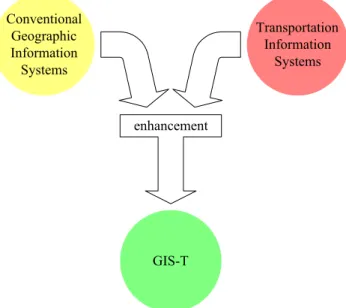
Geographic information systems for transportation (GIS-T) are the result of the integration of transportation information systems and conventional geographic information systems [Thill 2000] (Figure 1). According to [Vonderohe et al. 1993, p. 2], “GIS is much more than a tool to be applied case by case to a narrow set of specialized problems. Because of the inherent geographic nature of almost all transportation data, GIS concepts can and should serve as bases for the coherent organization of information structures and systems across the entire range of
transportation applications. GIS provides a framework for moving from stand-alone isolated databases and applications to truly integrated information systems”.
Conventional Geographic Information Systems Transportation Information Systems GIS-T enhancement
Figure 1 - GIS-T as the result of the union of and enhanced TIS and an enhanced GIS. Source: [Vonderohe et al. 1993]
Within the GIS and GIS-T functional context, [Vonderohe et al. 1993] presented six general categories of functions for data manipulation and spatial analysis: measurement, proximity analysis, raster processing, surface model generation and analysis, network analysis, and polygon overlay. Regarding constraint management in route planning and selection, this research is basically placed in the network analysis category, which is composed of two analysis functions: dynamic segmentation and network overlay. According to [Pereira et al. 2002a], constraint management becomes more complex when route planning takes into account an integrated public transportation network (i.e. a multimodal network).
In order to implement the proposed constraint management module, a study on the pedestrian’s behavioral impedance has been developed, which is composed of the analytical and mathematical approaches [Pereira et al. 2001, p. 279]. According to the authors, “the term behavioral impedance (BI) is used to refer to the constraints universe related to route planning techniques”.
There have been few studies where the constraint domain for a pedestrian in an urban transportation system was clearly stated. In this context, [Ahern 2001] presented a study on decision-making process where the Theory of Planned Behavior plays an important role. [Shriver 1997] argued that the pedestrian environment aspects constrain or facilitate a pedestrian trip. The author also commented on the limited analysis of travel distance and critical aspects of pedestrian behavior in research on walking.
More studies need to be carried out to ascertain the BI domain in transportation network systems from the pedestrian’s perspective, which is an open approach yet. The goal of this paper is to present the BI constraint management module from the pedestrian’s perspective within the urban public transportation context. The BI constraint management module has been implemented in Visual C++ 6.0 and a commercial GIS (i.e. Geomedia 4.0) has been used to support the map objects.
The structure of the paper is as follows. Section 2 reviews the behavioral impedance domain, which is composed of a meta-model, a taxonomy and a cost function mathematical model.
Section 3 present a complete description of the BI constraint management module, in which the BIRPA algorithm (i.e. behavioral impedance route planning algorithm) is included. Section 4 surveys the performance results and some considerations on BI constraint management module. Section 5 provides the conclusions and points out future research activities.
2 Behavioral Impedance Domain: A Brief Review
In a transportation network, behavioral impedance (BI) means a specific resistance imposed to the user on a part or whole transportation system. Thus, several objective (e.g. hard acclivities) and subjective (e.g. confort) criteria will play an important role in the transportation system. The BI domain has been developed using a meta-model as a starting point, which has allowed to establish the proposed taxonomy elements. Thus, the meta-model has allowed not only the classification and decomposition of the taxonomy elements, but also the identification of several constraints related to the BI domain [Pereira et al. 2001].
2.1 Meta-model
Taking into account that a meta-model represents the primary knowledge source that supports the identification of the appropriate constraints and dependency relations in a specific problem [Raghunathan 1992], [Pereira et al. 2001] have presented the BI meta-model structure (Figure 2). This meta-model is composed of analytical and mathematical approaches. The analytical approach of the meta-model is used to define the tree of the BI taxonomy. On the other hand, the mathematical approach is used to specify the constraint values that will be applied to the cost function mathematical model implemented in the BI constraint management module.
Entity State Condition Constraint An alytica l A pp roa ch Mat hema tic al Ap pr oa ch contains holds entails
Figure 2 - Meta-model of the Behavioral Impedance Domain. Source: [Pereira et al. 2001]. The meta-model has also been organized as a hierarchy composed of four levels: Entity, State, Condition and Constraint. The analytical approach has the Entity, State and Conditions levels (i.e. three first levels). The Mathematical approach deal with the Constraints (i.e. fourth level).
2.2 Reviewed taxonomy
The revised taxonomy presented in the Figure 3 consists of (1) some complex structural rules based on behavioral constraints of pedestrians; (2) a correspondence between the representation order from the meta-model's elements and the order observed in the real occurrences; (3) a taxonomy scheme that avoids arbitrary elements; and (4) some validation criteria based on research findings from the specialized literature and the results of a questionnaire submitted to a sample of people at the Technical University of Catalonia.
Behavioral Impedance Domain Environment
Topographic Weather
Permanent Temporary Sun Rain SnowHailFog Cataclysm
Socio-politico-economic Safety Policy Traffic flow Reliability Fare system Security Dangerous zones Strategic Operational Free Subsidiary Network Incidental Infra-structure Accidental Intentional Accessibility
Not programed Not programed Programed Simulated Real Change Facility Possibility Connectivity Schedule User Personal Professional
Comfort Emergency Schedule
Urgent Not urgent
Availability Emergency Urgent Not urgent Disability
Physical Psychological
Temporal (Day)
Work day Peak hour Off-peak
(Period)
Among-peak
Weekend /Holiday
(Period) Atypical day(Period) Peak hour Off-peak
Among-peak
Peak hour Off-peak
Among-peak
Headway Reliability system
Figure 3 - Taxonomy of behavioral impedance domain. Source: [Pereira et al. 2002a].
Using the BI domain analytical approach as a starting point, the cost function mathematical model has been developed [Pereira et al. 2002b]. The BI formulation consists of adding a BI weight (for each candidate to best path using the BI weights of each link) to the usual cost measure (i.e. time or distance, or both). Assuming a directly graph (i.e. transportation network)
[
,]
G= N A , it defines J as the set of all path identifiers of G. The total cost function is:
(
) (
)
1(
)
Total j j BI j
C Path =C Path ⋅ + C Path (1)
where: C Path
(
j)
is an usual cost measure function such as time or distance;(
)
BI j
C Path is the BI cost function that takes into account the transportation system’s and user’s data.
Assuming po as the origin point and pd as the destination point, J'⊂J is the set of possible path identifiers between po and pd, dmin and dmax are respectively the minimum and maximum travel distances in
J
', andmin
t and tmax are respectively the minimum and maximum travel times in
J
', the following equation represents the general formula to select the optimum path taking into account the BI domain:(
)
*
Total j
j J
Path Min C Path
∈
subject to:
(
)
(
)
(
)
'min BI j Total j max BI j ;
d ⋅C Path ≤C Path ≤d ⋅C Path ∀ ∈ j J
(
)
(
)
(
)
'min BI j Total j max BI j ;
t ⋅C Path ≤C Path ≤t ⋅C Path ∀ ∈ j J
More details about de BI mathematical formulation can be found in [Pereira et al. 2002b]. The authors also comment on the BI domain validation from the statistical analysis results, which are based on the partial least squares (PLS) approach.
3. BI Constraint Management Module
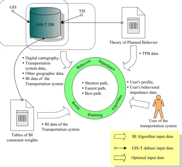
Using the cost function mathematical model presented above, the constraint management module architecture (Figure 4) is designed to be attached to the owner applications that work with geographic data as well as GIS-T.
text textGIS-T DB TIS GIS User of the transportation system y Digital cartography, y Transportation system data,
y Other geographic data, y BI data of the
Transportation system y User's profile,
y User's behavioral impedance data. Theory of Planned Behavior y TPB data Ro ute Behav ior Impe dance Planning Alg orith m y Shortest path, y Fastest path, y Best path. Tables of BI constraint weights y BI data of the Transportation system
Optional input data BI Algorithm input data GIS-T dabase input data
Figure 4 – BI Constraint management module architecture
The constraint management module architecture is composed of a main engine characterized by the behavioral impedance route planning algorithm (BIRPA). BIRPA algorithm has two primary data providers (i.e. GIS-T database and users of the transportation system) and two secondary data providers (i.e. weight table of the BI constraints and data from the theory of planned behavior).
3.1 Data of the GIS-T database
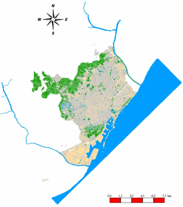
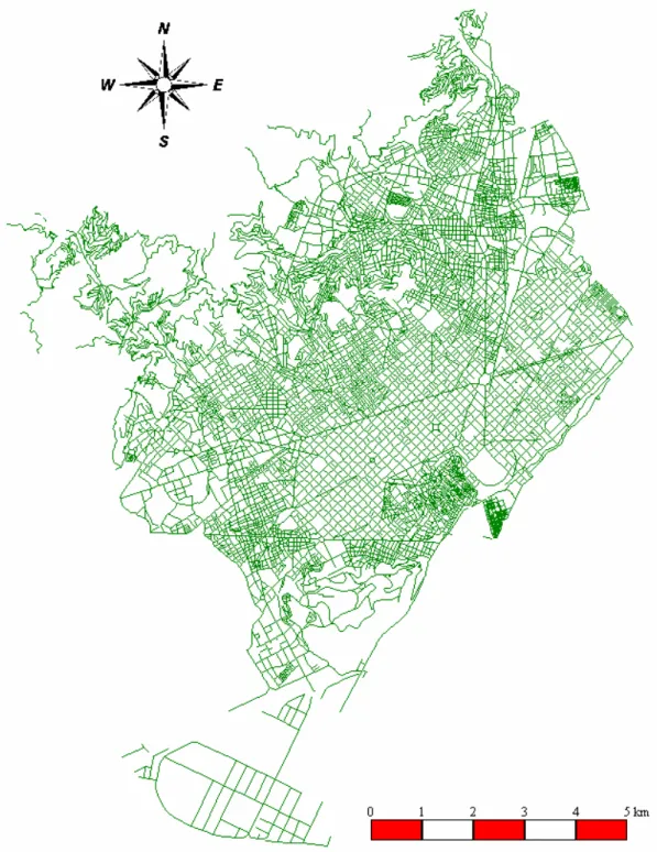
In this study, the Barcelona transportation system is used in order to implement the BIRPA. The digital cartography of Barcelona was facilitated by its Town Council through the Computer Municipal Institute (Instituto Minicipal de Informática - IMI). The GIS-T database is composed of (1) graphical files (i.e. those that allow visualize geographical characteristics, urban equipment and some cadastral data) and (2) alphanumeric files (i.e. those that contain all descriptive information on the graphical files content) . Figure 5 presents the digital cartography of Barcelona and Figure 6 shows the graph used by BIRPA algorithm, which represents the path layer of Barcelona.
Figure 5 – Digital cartography of Barcelona city. Source: Town Council of Barcelona and Computer Municipal Institute
Figure 6 – Path layer graph of Barcelona city. Source: Town Council of Barcelona and Computer Municipal Institute
3.2 Data of the user of the transportation system
This kind of datum refers to the user’s profile and the BI information determined by user. On the one hand, the user’s profile consists of a set of pattern information about the personal characteristics of each user (e.g. user’s disability or his/her usual travel motive). Moreover,
these informations can be saved by the owner applications or GIS-T for them reuse later. On the other hand, the BI informations are easily assigned by the users during the path selection process. In this way, the user can change them until the best path according to his/her needs is found (e.g. to fit the weather condition data or the change quantity that the user is ready to do). The data defined by the user is saved in the user’s profile tables (UPT), which are shown in Figure 7.
Field Type Characteristics --- GROUP CHAR(20) PRIMARY KEY
ID_PERSON AUTONUMERIC PRIMARY KEY, FOREING KEY BIEW01 NUMERIC(1,4) VALUE IN [0,1]
. . .
. . .
. . .
BIEW08 NUMERIC(1,4) VALUE IN [0,1] BITW09 NUMERIC(1,4) VALUE IN [0,1]
. . .
. . .
. . .
BITW17 NUMERIC(1,4) VALUE IN [0,1] BINW18 NUMERIC(1,4) VALUE IN [0,1]
. . .
. . .
. . .
BINW23 NUMERIC(1,4) VALUE IN [0,1] BIUW24 NUMERIC(1,4) VALUE IN [0,1]
. . .
. . .
. . .
BIUW29 NUMERIC(1,4) VALUE IN [0,1] BISPEW30 NUMERIC(1,4) VALUE IN [0,1]
. . .
. . .
. . .
BISPEW36 NUMERIC(1,4) VALUE IN [0,1]
a) User’s BI conditions table
Field Type Characteristics --- ID_PERSON AUTONUMERIC PRIMARY KEY
RG_PERSON CHAR(15) F_NAME CHAR(20) M_NAME CHAR(20) L_NAME CHAR(20) BIRTHDAY DATE F_REGISTER DATE L_UPDATE DATE
QT_CHANGE NUMERIC(3,0) VALUE IN [1,n]
b) User’s personal data table Figure 7 - User’s profile tables
The UPT tables are linked by the ID_PERSON attribute. The first row of the UPT table is defined as basic user’s profile (BUP) because the algorithm BIRPA uses a user’s profile to load the data structure in RAM memory. This procedure allows to reduce the path computation because the data load is performed during the start up process of the application (see Section 3.5).
3.3 Data of the theory of planned behavior
The study of the BI domain entails a behavioral analysis of the people’s intentions throughout the route selection process within a multimodal public transportation system. Such requirement
must be based on a theoretical foundation. In this way, the theory of planned behavior (TPB) is the more adequate theoretical foundation with respect to the BI domain. TPB is also used to define possible user’s behavioral profiles.
The TPB is based on the theory of reasoned action, which is addressed to the conception of intention during the performance of a determined behavior allowing the prediction and explanation of a goal-directed behavior [Ajzen 1985]. Thus, the TPB takes into account the actual and perceived control of the behavior that is being studied.
The TPB is a theory focused on the study of human behavior from behavioral, normative and control beliefs. In this way, the TPB enables to predict and explain the goal-directed human behavior. The TPB, thus, consists of a schema that traces the causal links from beliefs to behavior through three factors: attitudes (A), subjective norms (SN) and perceived behavioral control (PBC) (Figure 8). These factors lead to the formation of the individual’s intention, which is one of the central factors of the TPB to perform a given behavior [Ajzen 1991, 2001]. According to [Armitage and Conner 1999, p. 35], the “intention is regarded as the motivation necessary to engage in a particular behaviour: the more one intends to engage in a behaviour, the more likely should be its performance”.
Attitude toward the behavior Subjective norm Perceived behavioral control Intention Behavior
Figure 8 - Theory of Planned Behavior. Source: [Ajzen 1991]
Figure 8 not only depicts the TPB theoretical construction but also the relationships among theirs components. Equation 3 mathematically represents the TPB:
[
1 2 3]
~
B I∝ w A w SN w PBC+ + (3)
where B represents the behavior of interest, I is the person’s intention to perform behavior B and
w1, w2 and w3 are weights empirically determined that point out the relative importance of A, SN and PBC, respectively [Ajzen 1985, 1991].
Within this context, the data obtained from the TPB analysis are used to define (1) the user’s profiles in order to support the user of the transportation system during the work with constraint management module, and (2) the weights used in the selection of transportation mode. In addition, the data obtained from TPB analysis can be used to establish new strategy policies.
3.4 Data of the BI weight table
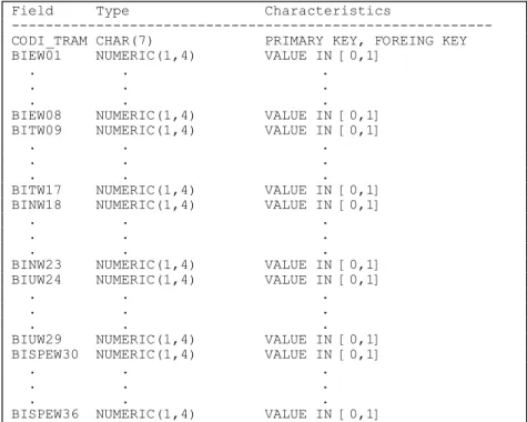
transportation system. Regarding this research’s context, the users are pedestrian. In order to obtain relevant BI values, it is recommended applying questionnaires to each sector of the study area, in which the transportation system is placed. Figure 9 shows the BI weight table added to GIS-T database.
Field Type Characteristics
--- CODI_TRAM CHAR(7) PRIMARY KEY, FOREING KEY BIEW01 NUMERIC(1,4) VALUE IN [0,1]
. . .
. . .
. . .
BIEW08 NUMERIC(1,4) VALUE IN [0,1] BITW09 NUMERIC(1,4) VALUE IN [0,1]
. . .
. . .
. . .
BITW17 NUMERIC(1,4) VALUE IN [0,1] BINW18 NUMERIC(1,4) VALUE IN [0,1]
. . .
. . .
. . .
BINW23 NUMERIC(1,4) VALUE IN [0,1] BIUW24 NUMERIC(1,4) VALUE IN [0,1]
. . .
. . .
. . .
BIUW29 NUMERIC(1,4) VALUE IN [0,1] BISPEW30 NUMERIC(1,4) VALUE IN [0,1]
. . .
. . .
. . .
BISPEW36 NUMERIC(1,4) VALUE IN [0,1]
Figure 9 - BI weight table structure
BI weight table is composed of thirty-seven attributes. The first one is the link code that allows the deduction of the relation with the links table and guarantee the referential integrity. The other attributes represent the BI conditions, in which the constraint coefficients are assigned.
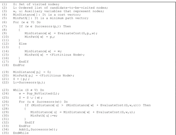
3.5 BIRPA Algorithm
Using the structure of the BI constraint management module presented above as a starting point, the behavioral impedance route planning algorithm (BIRPA) is implemented. The BIRPA algorithm is a modified version of Dijkstra’s algorithm [Dijkstra 1959].
The data structure and algorithm have been defined and optimized in order to obtain a fast computation time during the route selection process. Regarding the data magnitude (i.e. a digraph with approximately 9000 nodes and 27000 arcs, which represents the path layer of Barcelona), the digraph should be loaded in RAM memory to avoid some problems such as timeout (i.e. when the BIRPA algorithm is working on WEB) or unaceptable response times. The use of the RAM memory by the BIRPA algorithm (Barcelona digital cartography and auxiliary access structures) is less than 14 MBytes.
3.5.1 Data structure and algorithm
As commented, the main requirement is the path computation time. In this way, the proposed data structure (Figure 9) implies an expensive building process (i.e. loading time and resources). However, this building process is only performed once during the system’s start up implying a reduction in the path computation time for each route.
The data structure uses adjacency lists to represent the digraph and is defined as follows. First, there is a head that contains N (where N is configurable) grouped node lists (GNL). The nodes are ordered from smaller one to bigger one within each list and among them. The lists’ length is identical, except the last one, which length can be smaller.
Each list is composed of three elements: the number of nodes of the list, the last GNL node identifier and a pointer to the corresponding first GNL node. This structure allows a quick data loading and fast path computation. For instance, to find node “8999”, the algorithm would be forced to iterate in a single structure 8999 times. On the other hand, the use of GNL lists decreases the number of iterations (i.e. the number of verifications) performed until a specific GNL node is found.
The proposed solution performes (1) a dichotomic search in the GNL lists in order to identify the GNL sub-list where specific GNL node is placed and (2) a sequential search into the found GNL sub-list. In this way, the decrease of the search time is guaranteed increasing the data-loading and path-computation performance.
Each origin node has a ordered list of arcs from smaller to bigger real distance or relative travel time. Each arc is linked to its destination (or target) node through a pointer of memory.
Node Node Node Node Arc Arc Arc 1 2 3 1: Node information 2: Pointer to the arcs list
3: Successor
1 2 3 Arc
1: Arc information 2: Pointer to the arc successor
3: Pointer to the target node Grouped node list (GNL) 1 2 3 GNL 1: Number of nodes 2: Last GNL ID 3: Pointer to the each first GNL element
Node
Node Node Node
Node Node
...
... ...
Figure 9 - Data structure used in BIRPA algorithm
Despite of the fact that the whole digital cartography loading takes six minutes, some improvements have been made to increase the BIRPA algorithm performance in terms of data load speed and path computation time.
Considering G the digraph that represents the path layer, V the set of nodes and A the set of arcs, where G=( , )V A , the origin and destination points of a selected route are defined as po and
d
p respectively. In this way, BIRPA algorithm is defined as follows:
Step 1: For ∀ ∈w V, verify if w pertains to the origin node successors po. If yes, it assigns the calculated cost to the w-position of the cost vector, and assigns the po node to the w-position of the minimum path vector, where ∀ ∃V f V: ←→ . If not, assigns
∞value to the w-position of the cost vector and a fictitious node to the w-position of the minimum path vector. In addition, some variables are initialized.
Step 2: Considering S V≠ , while all nodes have not been visited, the next node to visit (v) is obtained from the candidate-to-be-visited list (L). Next, the obtained node is added to the visited node list (S).
Step 2.1: For the successors of the obtained node (v), verify if the cost of the path through the v is less than the current cost to visit the node u (i.e. one of the v successors). If yes, it assigns the current cost of the path through the u to the
u-position of the cost vector. If not, it maintains the current cost.
Step 2.2: Add in order the u successors to the L list, which path goes through v.
Step 3: Verify if po = pd. If yes, there is no path. If not, go through the minimum path vector from pd until po, obtaining all the nodes that are part of the selected path.
(1) S: Set of visited nodes;
(2) L: Ordered list of candidate-to-be-visited nodes; (3) w, u: Auxiliary variables that represent nodes; (4) MinDistance[]: It is a cost vector;
(5) MinPath[]: It is a minimum path vector; (6) For (w ∈ V) Do (7) If (w ∈ Succesors(po)) Then (8) { (9) MinDistance[w] = EvaluateCost(G,po,w); (10) MinPath[w] = po; (11) } (12) Else (13) { (14) MinDistance[w] = ∞;
(15) MinPath[w] = <Fictitious Node>; (16) }
(17) EndIf (18) EndFor
(19) MinDistance[po] = 0;
(20) MinPath[po] = <Fictitious Node>;
(21) S = {po}; (22) L:=Succesors(po); (23) While (S ≠ V) Do (24) w = Pop_NoVisited(L); (25) S = S ∪ {w}; (26) For (u ∈ Succesors(w)) Do
(27) If (MinDistance[u] > (MinDistance[w] + EvaluateCost(G,w,u))) Then (28) {
(29) MinDistance[u] = MinDistance[w] + EvaluateCost(G,w,u); (30) MinPath[u]:=w; (31) } (32) EndIf (33) EndFor (34) Add(L,Succesors(w)); (35) EndWhile
Figure 10 - BIRPA algorithm
Once the BIRPA algorithm is executed, the path is saved within the data structure placed in RAM memory (i.e. a minimum path vector). The path can be easily recovered by the recovery function shown in Figure 11 (Step 3 commented above).
(1) If po == pd Then (2) { (3) Write(po); (4) } (5) Else (6) { (7) While (po ≠ pd) (8) Write(pd); (9) pd = MinPath[pd]; (10) EndWhile (11) } (12) Write(pd);
Figure 11 – Recovery function of BIRPA algorithm
4 Performance Results and Some Considerations
Basic version of Dijkstra’s algorithm, in which there are a data structure and a not-optimal algorithm, can produce a high temporal cost. BI proposal is developed to run in on-line systems. Within this context, temporal costs are studied in order to improve and opmitize BIRPA algorithm.
The main temporal cost criteria analized are (1) quantity of iterations to visit all nodes, (2) determination of the next node to visit and (3) access to the node successors. The first cost criteria is unavoidable due to unreliable results. The second one is partially avoidable depending on how the digraph is composed (e.g. the average number of connections among nodes). Finally, the third one is avoidable using a well-defined data structure.
The asymptotic time complexity of the BIRPA algorithm is O n
( )
2 and is equivalent to Dijkstra’s algorithm complexity. To determine this computational cost, three BI algorithm versions have been designed. The computation cost of the BI algorithm is the same for all versions.• Version 1 – Non-optimized data structure and algorithm: In this case, there are neither complexity data structure nor a data pre-process. The algorithm is not optimized and the temporal costs presented above are not solved. The computation time of the minimum path is of the order of some minutes.
• Version 2 – Optimized data structure and non-optimized algorithm: In this case, there is a complex data structure and data pre-process. The algorithm is not optimized and the temporal cost taking into account third criterion is solved. The computation time of the minimum path is 11 seconds for any path.
• Version 3 – Optimized data structure and algorithm: In this case, there is a complex data structure and a data pre-process. Moreover, the algorithm is optimized by a structure of identifiers, which point out the next node to visit. The second criterion of the temporal cost is solved. The computation time of the minimum path is 0.076 seconds for any path. Therefore, the decrease of computation time from minutes (version 1) to seconds (version 2) justifies the data pre-process. In addition, the use of auxiliary structures is justified due to the decrease of computation time from seconds (version 2) to hundredths of a second (version 3).
5 Concluding remarks
In this paper, a review of the behavioral impedance domain has been presented. The BI domain is initially proposed by [Pereira et al. 2001] and validated in [Pereira et al. 2002a, 2002b]. The constraint management module has also been presented, which is based on the BI domain. The
module’s goal is the possible attachment to owner applications that manipulate geographic information or GIS-T in order to offer to the pedestrian better alternatives of trip.
Future activities of research will consist of simulating the BI path calculus for different user’s profiles (e.g. cyclists) and improving the calculus time of BIRPA as stand alone applications, for instance as WEB applications.
Acknowledgements
This research has been partially supported by the CICYT under the project TIC2001-2099-C03-01.
Referências
Ahern, A. A., “Modal choices and new urban public transport”, Traffic Engineering & Control, 42, 4 (2001), pp. 108-114.
Ajzen, I., “From intentions to actions: A theory of planned behavior”, In J. Kuhl & J. Beckman (Eds.), Action-control: From cognition to behavior, pp. 11-39, Heidelberg: Springer, 1985.
Ajzen, I., “The theory of planned behavior”, Organizational Behavior and Human Decision
Processes, 50 (1991), pp. 179-211.
Ajzen, I., “Constructing a TpB Questionnaire: Conceptual and Methodological Considerations”, December (2001), pp. 1-14.
* http://www-unix.oit.umass.edu/~aizen/pdf/tpb.measurement.pdf
Armitage, C. J. and Conner, M., “The theory of planned behavior: Assessment of predictive validity and ‘perceived control’”, British Journal of Social Psychology, 38 (1999), pp. 35-54.
Dijkstra, E. W., “A Note on Two Problems in Connexion with Graphs”. Numerische
Mathematik, 1 (1959), pp. 269-271.
Pereira, H. B. B., Nogueira, D. L. and Pérez, Ll. V., “Behavioral impedance for route planning techniques from the pedestrian’s perspective: Theoretical contextualization and taxonomy”, Anais do XV ANPET – Congresso de Pesquisa e Ensino em Transportes,
ANPET, Campinas, Relatórios de Teses e Dissertações em Andamento – Comunicações
Técnicas, 2001, pp. 277-283.
Pereira, H. B. B., Nogueira, D. L. and Pérez, Ll. V., “Considerations on Constraint Management for Pedestrian’s Route Selection in Geographic Information System for Transportation”,
Anais do III CONGRESO INTERNACIONAL GEOMATICA 2002, La Habana, Fevereiro,
2002a.
Pereira, H. B. B., Pérez, Ll. V., Nogueira, D. L. and Bohórquez, M. M. “Domínio da impedância comportamental: desenvolvendo a abordagem matemática”, Submitted to the
XVI ANPET – Congresso de Pesquisa e Ensino em Transportes, ANPET, Natal, 2002b.
Raghunathan, S., “A Planning Aid: An Intelligent Modeling System for Planning Problems Based on Constraint Satisfaction”, IEEE Transactions on Knowledge and Data
Engineering, 4, 4 (1992), pp. 317-335.
Shriver, K., “Influence of Environmental Design on Pedestrian Travel Behavior in Four Austin Neighborhoods”, Transportation Research Record, 1578 (1997), pp. 64-75.
Thill, J. C., “Geographic information systems for transportation in perspective”, Transportation
Research, Part C, 8, 1-6 (2000), pp. 3-12.
Vonderohe, A. P., Travis, L., Smith, R. L. and Tsai, V., Adaptation of Geographic Information
System for Transportation, Transportation Research Board, NCHRP Report 359. National
![Figure 2 - Meta-model of the Behavioral Impedance Domain. Source: [Pereira et al. 2001]](https://thumb-eu.123doks.com/thumbv2/123dok_br/17031842.766813/3.918.361.562.585.893/figure-meta-model-behavioral-impedance-domain-source-pereira.webp)
![Figure 3 - Taxonomy of behavioral impedance domain. Source: [Pereira et al. 2002a].](https://thumb-eu.123doks.com/thumbv2/123dok_br/17031842.766813/4.918.166.751.279.611/figure-taxonomy-behavioral-impedance-domain-source-pereira-et.webp)
![Figure 8 - Theory of Planned Behavior. Source: [Ajzen 1991]](https://thumb-eu.123doks.com/thumbv2/123dok_br/17031842.766813/9.918.317.626.441.721/figure-theory-planned-behavior-source-ajzen.webp)