Causal characterization of functional connectivity through the spread of electrically induced oscillations in the epileptic human brain

(1)

Miguel Fernandes Duarte

Licenciado em Ciências de Engenharia Biomédica

Causal characterization of functional

connectivity through the spread of

electrically induced oscillations in the

epileptic human brain

Dissertação para a obtenção do Grau de Mestre em

Engenharia Biomédica

Orientador: Antoni Valéro-Cabré, MD PhD,

Institut du Cérveau et de la Moèlle Épinière

Co-orientador: Julià L. Amengual, PhD,

Institut du Cérveau et de la Moèlle Épinière

Co-orientador: Carla Quintão, PhD,

Faculdade de Ciências e Tecnologias da Universidade Nova de Lisboa

Júri:

Presidente: José Luís Ferreira, PhD,

Arguente: Ricardo Vigário, PhD,

Vogal: Carla Quintão, PhD,

(2)

(3)

Miguel Fernandes Duarte

Licenciado em Ciências de Engenharia Biomédica

Causal characterization of functional

connectivity through the spread of

electrically induced oscillations in the

epileptic human brain

Dissertação para a obtenção do Grau de Mestre em

Engenharia Biomédica

Orientador: Antoni Valéro-Cabré, MD PhD, Institut du Cérveau et de la Moèlle Épinière

Co-orientador: Julià L. Amengual, PhD, Institut du Cérveau et de la Moèlle Épinière

Co-orientador: Carla Quintão, PhD,

(4)

(5)

Causal characterization of functional connectivity through the spread of electrically in-duced oscillations in the epileptic human brain

(6)

(7)

Acknowledgements

This thesis would not be complete without the help of so many. To those at the Institut du Cérveau et de la Moélle Épinière (ICM) and speciﬁcally at the FrontLab, thank you for making me feel at ease and at home on the ﬁve months I spent there. In what regards the people of the ICM, I have to especially pay compliments to both my supervisors, Antoni Valéro-Cabré and Julià Améngual (whose baby made his work even tougher), who made everything in their reach to make this project as best as it could have been. I have also to thank the people from Université Paris Descartes and from the Bioengineering and Inovation in Neurosciences track at the Master in Biomedical Engineering in Paris, that taught me a lot during my stay.

To my friends at the Maison du Portugal, in Paris, whose help was essential in this period I was abroad, particularly from those that did eat a lot of Ramen. It’s food for thought. Without them, living in Paris would have been less beautiful, less fun, more sad.

To my good friends I made while studying at FCT-UNL (Alheiras, you know who I’m talking to), I can’t thank you enough for these whole ﬁve years we have all been through while completing this Master. Those years can’t be taken back and will always stay in my mind.

To my parents, my brother and my grandmother, whose preocupation and pledge for eﬀort made me want to ﬁnish this Master in the best possible manner.

(8)

(9)

Abstract

Little is known about the rules governing the spread of local entrainment within synchronized networks distributed across the brain. The assessment of the causal influences impacting in-formation flow between two brain regions have mainly relied on confirmatory model-driven ap-proaches (such as dynamic causal modeling and structural equation modeling) and exploratory data driven approaches (such as Granger Causality analysis). However, stimulation-driven ap-proaches offer a unique opportunity to impact ongoing brain activity and describe the causal consequences of such manipulations, performed on a specific node of a complex cerebral network. In this project, we characterize causal functional interactions between brain regions by assess-ing how frequency-tuned electrical currents delivered intracranially in awaken epileptic patients enhance inter-regional synchrony between pairs of areas.

To achieve this goal, we worked with an existing iEEG database from 18 medication-resistant epilepsy patients undergoing Intracortical Stimulation Mapping Procedures (ISMP) performed to causally identify and localize the epileptogenic foci, prior to neurosurgical removal. Patients are implanted with series of multi-electrodes in well-known brain regions under MRI guidance. Intracranial EEG contacts allow continuous recordings and the delivery through pairs of adjacent contacts of biphasic pulses of rhythmic Direct Electric Stimulations (DES) at a 50Hz frequency coupled to electrophysiological recordings.

Measuring signiﬁcant increases in gamma power ( 50Hz) observed during the stimulation period (vs. prior the stimulation), and signiﬁcant increases of Phase-Locking Value (PLV) be-tween signals recorded in the electrically stimulated regions and activity evoked in the rest of implanted regions during stimulation (vs. prior simulation), we characterize the spread of os-cillatory entrainment from the stimulated region to the remaining regions, thus establishing a network of functional connectivity in the brain. By comparing this network with the one shown during resting-state, we assess how entrainment to frequency-tuned electrical currents delivered intracranially is predicted by the resting-state functional connectivity network.

(10)

(11)

Resumo

Pouco é conhecido acerca das regras que governam a propagação de arrastamento (entrainment)

local em redes sincronizadas distribuídas ao longo do cérebro. A avaliação das influencias cau-sais que influenciam o fluxo de informação entre duas regiões cerebrais tem maioritariamente dependido em abordagens confirmatórias usando modelos (como dynamical causal modeling e structural equation modeling) ou através de abordagens de exploração de dados (como análises da

causalidade de Granger). No entanto, as abordagens através de estimulação oferecem a oportu-nidade única de inﬂuenciar a actividade cerebral em andamento e de descrever as consequências causais dessas manipulações, feitas em nós especíﬁcos de uma complexa rede cerebral.

Neste projecto, caracterizamos as interacções funcionais causais entre regiões cerebrais, avaliando como a sincronia inter-regional entre pares de regiões cerebrais é modiﬁcada quando sujeitas a correntes eléctricas de 50Hz, administradas intracranianamente em pacientes epilép-ticos acordados.

Utilizámos uma já existente base-de-dados de iEEG adquirida em 18 pacientes epilépti-cos resistentes à medicação, quando estes foram submetidos a estimulações intracorticais para, causalmente, identiﬁcar e localizar o foco epileptogénico, de modo a ser retirado. Para tal, os pacientes são implantados com séries de multi-eléctrodos em regiões cerebrais identiﬁcadas e determinadas clinicamente.

Os contactos do EEG intracranial permitem a gravação contínua e a libertação, através de pares de contactos adjacentes, de rítmicos pulsos bifásicos de Estimulação Eléctrica Directa (EED), a uma frequência de 50Hz.

Medindo aumentos signiﬁcativos de potência gama ( 50Hz) observadas durante o período de estimulação (vs. antes da estimulação), e aumentos signiﬁcativos de Phase-Locking Value,

caracterizamos a propagação do arrastamento oscilatório da região estimulada para as restantes. Assim, estabelecemos uma rede de conectividade cerebral no cérebro. Ao comparar esta rede com a manifestada durante o estado de repouso, avaliamos de que forma o arrastamento a correntes eléctricas de 50Hz libertadas intracranialmente é previsto pela rede de conectividade funcional em estado de repouso.

(12)

(13)

List of Figures

Page

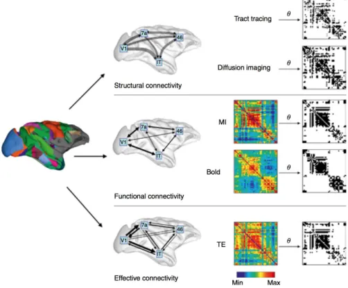
1.1 Structural, functional, and effective brain connectivity. The image on the left displays a rendering of the parcelated macaque cortical surface, the middle col-umn of plots shows schematic diagrams of structural connectivity (white matter pathways structurally linking brain regions), functional connectivity (statistical relations among brain regions), and effective connectivity (directed influences be-tween brain regions). Plots on the right show weighted (in colour) and thresholded binary (black/white) matrices of structural, functional, and effective connectivity patterns[1]_{. . . .} ₄

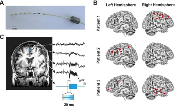
1.2 Example of multielectrode implantations and intracranial stimulation procedures. (A) Image of an 8-contact intracranial multielectrode employed for stimulation and iEEG recordings. (B) Diagram of the implantation sites showing the loca-tion of every individual multielectrode in the brain of three single patients. (C) Detailed caption of a single multielectrode implanted in the frontal lobe of one of these patients, displayed on a T1 MRI scan (coronal view) recorded following implantation. Blue dots represent pairs of electrode contacts delivering 5 seconds long 50 Hz electrical bursts (blue iEEG trace). White dots signal the location of remaining contacts within the same electrode, recording brain iEEG activity concurrently with electrical stimulation patterns[2]_{. . . .} ₈

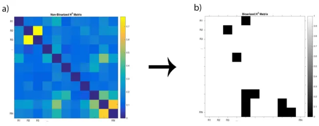
2.1 Regions comprising the AAL Atlas . . . 14 2.2 (a) example of a weighted adjacency matrix for h2 values, in which every

pair-wise edge has a value from 0 to 1. The diagonal of the matrix is set to 0, and represents the pair-wise edge between the pairs of the same region; (b) example of the adjacency matrix from the same dataset shown in (a) after thresholding and binarization, where the only values left are the ones that represent a meaningful connection (and are all set to 1) and every other value is 0. . . 16 2.3 Method applied to determine mean S-PLV representative for the pre-stimulation

(16)

Thesis LIST OF FIGURES

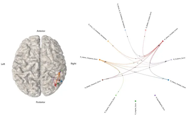
3.1 High Intensity Stimulation iEEG-based connectome, from patient reference 1998

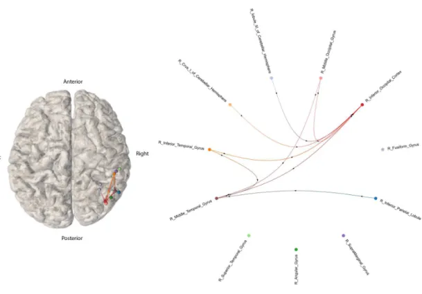
(n=1) displayed on a normalized brain volume or as a graph, estimated with S-PLVs. (Left panel) 3D connectome is represented in a normalized brain template, with each node corresponding to an implanted AAL region. The geometrical loca-tion of each node is placed on the average MNI localoca-tion of the contacts that were localized as located in the same AAL region. (Right panel) Connectome repre-sented as a circular graph with all nodes located equidistantly (importantly, nei-ther node location or edge length inform about the distance between two nodes). Nodes correspond to each implanted AAL region. In both graphs, arrows added to each edge represent the estimated direction of the signal spread from the elec-trically stimulated region to a second one. . . 22 3.2 Low Intensity Stimulation iEEG-based connectome, from patient reference 1998

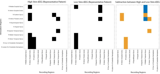
(n=1) based on S-PLVs. On the left side, a 3D connectome is represented in a default intact brain template in normalized space, with each node corresponding to an implanted AAL regions. The geometrical MNI node location represents the average x, y and z coordinates of the contacts hosted on the same AAL region. On the right side, the connectome is represented via a circular graph. Nodes correspond to each implanted AAL region. On both graphs, arrows in the edges represent the estimated direction of the signal spread (see caption from prior ﬁgure for further explanations or details) . . . 23 3.3 Comparison of adjacency matrices for patient ref. 1998 (n=1) based on S-PLVs. In

(a, left, in black) and (b, center, in black), edges are represented in black, whereas matrix (c, right) displays the edges present either only during high intensity stim-iEEG (orange cells) or exclusively during low intensity stim-stim-iEEG (blue cells). . . 24 3.4 Circular connectome with equidistally represented nodes, associated to prior

ad-jacency matrices based on S-PLVs for patient ref. 1998 (n=1), showing the edges present either only during high intensity stimulation iEEG datasets (in orange) or only during low intensity stimulation (in blue). . . 24 3.5 High Intensity Stimulation-iEEG Connectome Adjacency Matrix for the complete

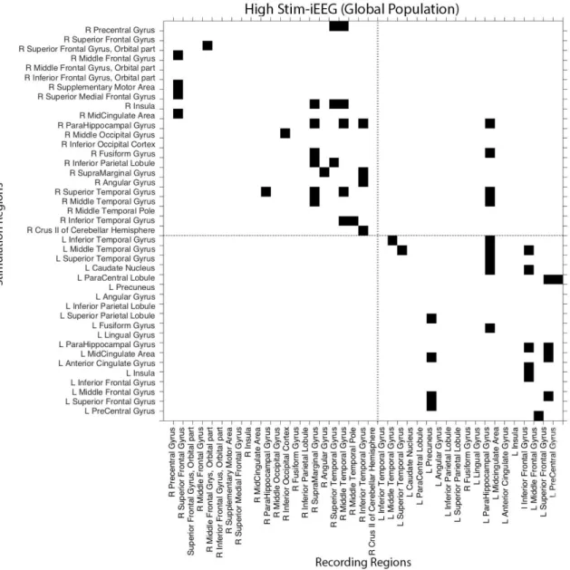
population of patients (n=18) based on S-PLVs. The horizontal and vertical dotted lines divide the brain regions belonging to the left or the right hemisphere. Black cells represent a pair-wise connection that fulﬁlled criterion for gamma (50 Hz) S-PLV increases during stimulation. . . 25 3.6 High Intensity Stimulation iEEG Connectomefor the entire population of subjects

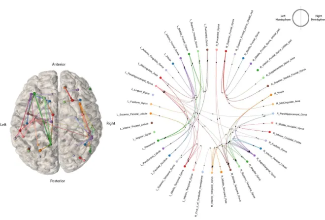
(n=18) analysed in our study based on S-PLV values. (Left panel) 3D connec-tome is represented in a default normalized brain template, in which each node corresponds to an implanted AAL region. Geometrical node location represents the average position of contacts belonging to the same AAL region. (Right panel) this population based connectome is represented in a circular graph with nodes placed equidistant to each other. Importantly, neither node location nor edge length inform about the distance between two nodes in the real anatomical space. Nodes signal the average MNI x, y, z coordinates of each implanted AAL regions across participants for a given AAL area. For both graphs, arrows present on the edges signal the estimated direction of activity spreads from a leading/driving site (the one receiving gamma stimulation bursts) towards ‘follower’ sites. . . 26 3.7 Low Intensity Stimulation iEEG-based Connectome Adjacency Matrix, integrating

data for the entire population of patients (n=18) based on S-PLVs. The horizontal and vertical dotted line divide brain regions of the left and the right hemisphere. Each black square represent a pair-wise connection. . . 27

(17)

3.8 Low Intensity Stimulation iEEG-based connectome, integrating data from the

en-tire population of patients (n=18). (Left panel), 3D connectome represented in a normalized MRI brain template, in which each node corresponds to an implanted AAL region. Node location represents the average x, y, z MNI coordinate position of the contacts belonging to the same AAL region. (Right panel), connectome represented with a circular graph, with standard equidistant nodes (hence non-informative on real intermodal length). Nodes correspond to implanted AAL region hosting at least a multielectrode contact. For both graphs, arrows dis-played on the edges represent the estimated direction of the iEEG signal spread driven by the stimulated region onto other brain regions. . . 28 3.9 Global connectome of the whole population of studied patients (n=18) showing

edges present only during high intensity stimulation-iEEG (in orange). . . 29 3.10 Global connectome integrating data from the entire population of patients

in-cluded in our study (n=18) displaying the edges present only during low intensity stimulation (in blue). . . 29 3.11 Resting state iEEG-based connectome for patient ref. 1998 (n=1). (Left panel)

3D rendering of the connectome, based for h2_xy, represented on a default and normalized MRI brain template, in which each nodes corresponds to the location of at least a contact implanted on an AAL region. Nodes are located on the average of x, y, z MNI coordinates of the diﬀerent contacts that are hosted in the same AAL region. (Right panel), h2_xy iEEG based resting state connectome represented on a circular graph in which nodes are depicted equidistantly. In both version of the graph (right and left), arrows depicted on the edges represent the estimated direction of the spread of the signal according to the value taken by the h2

xy. . . 30 3.12 Resting-State iEEG-based connectome matrix, for the entire population of

im-planted patients (n=18), according to the h2_xy measure. The horizontal and ver-tical dotted lines divide brain regions from the left and right hemispheres. Cells in black represent pair-wise connections. . . 31 3.13 Resting-State iEEG-based connectome, for the entire population of implanted

pa-tients (n=18), according to theh2

xy measure. (Left panel) 3D connectomic model represented in a normalized MRI brain template, in which each node corresponds to an implanted AAL regions hosting at least a recording contact. Node location signals the average x, y, z spatial coordinates of contacts hosted by the same AAL region. (Right panel), the connectome is represented on a circular graph made of equidistantly placed nodes, corresponding to each implanted AAL region. In both graphs, arrows displayed on each edge represent the estimated direction of signal ﬂow according to the values revealed by the h2

xy measure. . . 32 3.14 Resting-State iEEG-based connectome calculated with the S-PLV, for the entire

(18)

3.15 Resting-State iEEG-based connectome, for the entire population of patients dataset

(n=18) based on S-PLV measures. (Left panel), 3D connectome represented in a normalized MRI brain template, in which each node corresponds to contacts of an implanted AAL region. The location of each node is estimated as the average x, y, z coordinates of any contacts hosted in the same AAL region. (Right panel), connectome represented in a circular graph with equidistantly positioned nodes, corresponding to each implanted AAL region. In both graphs (Left and Right panels), arrows displayed on each edge represent the direction of the activity or the signal spread. . . 34 3.16 Connectome representation showing edges between nodes present only in the

Resting-State iEEG-based connectome using the S-PLV measures (in orange). . . 35

3.17 Connectome showing the edges present only during theResting-State iEEG-based connectome compiled on the basis of theh2

xy measure (in blue). . . 35 3.18 Connectome depictions showing the signiﬁcant edges or intermodal links present

only during gamma 50 Hz electrical stimulation (in orange) for the whole popu-lation of implanted patients studied in this work (n=18). . . 36 3.19 Connectome depictions showing the edges or links present only during resting

state interactions measured with iEEG (in blue). . . 37 3.20 Histogram of Node Degree values comparing data from the stimulation

iEEG-based connectome and the resting state iEEG-iEEG-based connectome. (Panel A, top left) shows node degree for both connectomes, with the higher bars indicating higher node degree for the node. (Panel B, top right) displays node degree dis-tribution data, from the lowest to highest node degree levels. (Panel C, bottom row) shows the diﬀerence in node degree between the two types of connectomes (Stim-iEEG and RS-iEEG), in descending order. Positive values signal brain ar-eas for which the node degree is higher on stimulation iEEG-based connectome than on the resting state iEEG-based connectome, whereas negative values signal the opposite. . . 38

(19)

List of Tables

Page

4.1 Summary table with demographic data (gender and age) of the patients (n=18) included in our analyses, the number of implanted multielectrodes, the total num-ber of contacts and the name of the cerebral regions covered by the implantations on each patient. F: Female; M: Male. . . 49 4.2 Summary table with demographic data (gender and age) of the patients (n=18)

(20)

(21)

Chapter 1

Introduction and State of the Art

The human brain remains the object of a long set of unanswered questions inquiring on how this organ operates and behaves. For more than a century, inﬂuenced by the notion of neural systems conceived as highly specialized local systems (each underlying speciﬁc cognitive operations), brain research focused in the study of local systems and interactions. Nonetheless, relatively recent work strongly suggests that the human brain integrates sets of local networks that build up onto more complex highly interconnected global systems, making “the one more than just the sum of its parts”.

Indeed, considering the brain as a modularly organized highly integrated system, brain con-nectivity has risen to become a highly inﬂuent topic, instrumental for the advancement of brain sciences and the treatment of its diseases and conditions.

One of the main emerging properties of neural systems and their connectivity is the ability to produce rhythmic patterns of activity. In continuity with the local vs. widespread conception of neural systems mentioned above, correlational evidence in humans suggests that high-level cognitive function strongly relays on coherent fluctuations of oscillatory patterns along widely synchronized brain networks. In these settings, neural rhythms are generated by the synchro-nized activation of local and/or widespread networks of neuronal populations, which have proven key to generate the coding mechanisms allowing flexible and efficient inter-regional communica-tion, subtending cognition and ultimately leading to human behaviour.

Unfortunately, the relation between local and widespread structural and functional networks with behaviour has been often addressed through correlational measures, such as resting state or task activated Electroencephalography (EEG), Magnetoencephalography (MEG) or functional Magnetic Resonance Imaging (fMRI) which are prone to epiphenomena, i.e., they often incur in the risk to consider as causally related, tasks- or state-irrelevant patterns of activity generated in speciﬁc brain locations (or across networks) as causally related to a given function, when they only happen to coincide in time and space.

(22)

Thesis CHAPTER 1. INTRODUCTION AND STATE OF THE ART

the potential inﬂuence of a brain condition such as epilepsy on normal cerebral excitability and coding dynamics, and biases in brain sampled regions, often focalized in temporal regions, in-tracranial stimulation perturbation approaches have the potential to overcome the above-stated focality limitations and uncertainties, if one can cumulate data from a suﬃciently large cohort of cases. Hence, we aim to compile and compare qualitatively functional connectivity patterns of the human brain on the basis of intracranial direct brain recordings at resting-state or during the delivery of 50 Hz direct intracranial stimulation.

1.1 Connectivity and Causality

Connectivity deals with the way in which activity patterns recorded in pairs of regions or sites are temporally related and how they interact dynamically over space and time. The conjunction of pair-wise connectivity interactions between all possible combinations of sampled sites can be combined to define a connectome. In the human brain, sites correspond to the different discreet brain regions from which recording can be focally measured. Three different subtypes of brain connectivity have been thus far defined (see Figure 1.1): Structural connectivity, Functional connectivity and Effective connectivity[3, 4].

Figure 1.1: Structural, functional, and effective brain connectivity. The image on the left displays a rendering of the parcelated macaque cortical surface, the middle column of plots shows schematic

diagrams of structural connectivity (white matter pathways structurally linking brain regions), functional connectivity (statistical relations among brain regions), and effective connectivity (directed influences between brain regions). Plots on the right show weighted (in colour) and thresholded binary

(black/white) matrices of structural, functional, and effective connectivity patterns[1]_.

Structural connectivity refers to the plan of physical anatomical white matter connections

linking different brain regions. White matter pathways and, their microstructural properties, can be quantified with magnetic resonance imaging (MRI), by using so-called diffusion weighted imaging (DWI) sequences. DWI datasets are analysed with diffusion tensor imaging (DTI), and

(23)

allow the characterization of the so-called structural connectome, integrated by nodes (speciﬁc brain regions acting as hubs) and links (white matter connections). DTI methods are insensitive to the directionality and do not inform in any way or manner about the level of functionality subtended by hard-wired anatomical projections. Therefore, they do not allow the extraction or inference of any meaningful functional information, neither do they uncover the features of the information ﬂow and coding patterns running across them.

Functional connectivity refers to the statistical dependencies between neural activities in

different brain regions regardless of their anatomical connectivity patterns. It can be character-ized from either spontaneous and/or during task-driven brain activity. It is typically measured with functional magnetic resonance imaging (fMRI), a technique that considers the dynamics of increases and decreases in blood oxygen level-dependent (BOLD) signals from vessels sup-plying blood essentially to brain gray matter areas. These methods allow the characterization of different types of functional extended brain systems (such as, for example, the Default Mode Network and its different subsets) based on the mutual correlation of activity across different brain regions. A limitation of fMRI neuroimaging approaches, however, is the low temporal res-olution at which we can measure these activations (in the order of 1 to several seconds), which is far slower than the time-scale at which a majority of neural mechanisms tend to occur (in the order of milliseconds).

Importantly, functional networks of interactions maintain a tight relationship with structural connectivity patterns, i.e., the structural connectome predicts the functional connectome. How-ever, such relationship is not always straightforward. Indeed, functional interactions between two brain regions are not always subtended by direct structural white matter pathways linking those regions, but associated to indirect multi-synaptic long-range projections between the two sites.

Functional connectivity maps provide a set of ‘mere’ statistical relationships between activ-ity patterns subtended by different brain regions, which are not necessarily causal. Indeed, a question that cannot be addressed with these procedures is to what extent the activity of two brain regions is crucial for information to flow into a network, other than being merely related statistically? What is the causal meaning of the statistical relationship? This question brings us to the concept ofeffective connectivity, which refers to the influence that neural systems hosted

in a given brain region exerts over a second one, either at microscopic (synaptic activity) or macroscopic (regional excitability or activity levels of cortical/subcortical sites) levels. There-fore, the concept of effective connectivity provides information on directionality. This critical measure allows, for example, to show that the effect that a brain area “A“ exerts over another brain area “B“ might not be necessarily the same that area “B” exerts onto area “A”. In a strict physical sense, causality relies on the identification of a cause and an effect, or, in other words, an event that originates (cause) a given response or a given consequence (effect) in general in a dose dependent (direct or inverse linear or non-linear) manner.

In a deterministic sense, the concept of causality can be either conceived in terms of temporal precedence and/or of physical inﬂuence. The temporal precedence-based deﬁnition of causality

between two regions establishes that the activation of one of these regions must be preceded by the activation of another region. Nonetheless a more reliable manner to explore causality with regards to the influence of a brain region into another cerebral site consists on perturbing the activity pattern of a given site and observe whether such intervention influences the activity of a second site with whom we suspect subtends a causal interaction. The fundamental differ-ence between these two definitions characterizes the different approaches employed to analyse causality. The temporal definition is the basis for the so-called Granger causality (see further explanations in the methods section of this dissertation). In contrast, the physical definition

stated above is related to the notions of intervention and control[5]_{, in which this work has been}

(24)

1.2 EEG as a measure of connectivity

Functional and effective connectivity have been mainly studied using neuroimaging methods based on MRI recordings, as stated before. Despite being characterized as provided with an outstanding spatial resolution (in the order of several mm depending on voxel size and the influence of MRI field strength), the temporal resolution of the MRI BOLD signal, which mimics the activity of the different brain areas, is too slow (few seconds, depending on brain area and the tasks performed) to reflect the real dynamics associated with neuronal activation and signalling mechanisms, operating at the millisecond level.

A method that can overcome this limitation is electroencephalography (EEG). Using this technique, it is possible to record the electrical activity emerging from synchronous activations of neuronal population. There are different approaches to record EEG activity from the brain. The most common consists in recording EEG activity from the scalp (scalp EEG). This tech-nique is performed through an electrode cap placed on the subject’s head surface. It is a quite standardized and mainstream method in experimental and clinical applications. Nonetheless, the quality of the signal is limited given its sensitivity to be contaminated by non-biological elec-trical activity present in the environment, and to field distortion in sources of biological activity generated by layers of non-cerebral tissues (such as arachnoid mater, dura matter, skull bone and other subcutaneous layers, as well as the cerebrospinal fluid). placed between the signal source and the scalp EEG electrode[6]_.

During the last decade, additional technological approaches have been developed to over-come these limitations and record more spatially accurate patterns of brain activity. One of these methods is subdural electrocorticography (ECoG), a technique that involves the place-ment through a rather large craniotomy of two-dimensional grids of electrodes, which lay like a blanket, in direct in contact with the pial surface of speciﬁc cortical regions[7]_{. To note that,}

in humans, this technique, due to a high risk of infections, only allows recording either during neurosurgical operations, or for very brief periods of time before having to be extracted.

Another method is stereoelectroencephalography (sEEG) or intracranial EEG (iEEG), which consists on the placement of multi-contact electrode leads penetrating the brain[8]_{. Intracranial}

EEG enables the recording of local ﬁeld potentials (LFP), i.e. compound potential product of the temporal and spatial summation of action potentials from clusters of neurons located in the vicinity of the contact. This approach is often used as a pre-surgical removal intervention in medication-resistant epilepsy patients, and allows for longer monitoring periods (1-2 weeks) than ECoG.

Independently of the specific method used to record EEG activity, measuring electrical activ-ity in the brain allows to explore the underlying frequencies of brain oscillations present within the recorded signal. Local or widespread events of tonic or sustained oscillatory activity and synchrony, operating at specific frequency bands and cerebral sites have been found to encode for different cognitive processes such as attention, motor planning and memory, among others.

1.3 Entrainment of Brain Oscillations

A detailed and accurate comprehension of oscillatory phenomena is paramount for the funda-mental and the clinical neurosciences. This is because neural oscillations and phase and/or frequency speciﬁc synchronization of cerebral sites within a network, can encode speciﬁc cog-nitive processes and behaviours, and be modulated through neural oscillatory entrainment, a procedure that consists in the progressive synchronization in time of an oscillation to an ex-ternal source of energy such as electrical or magnetic stimulation[9]_{. Entrainment generated by}

a single stimulation source may operate locally, although entrained activity might also travel

(25)

throughout extended networks and hence modulate brain connectivity across large networks. In a scientiﬁcally or medically relevant diagnostic/therapeutic domains, these procedures could be used to impact coding mechanisms tied to normal/abnormal cognitive operations in which the targeted systems are involved and drive behavioural improvements For this reason, the de-velopment of non-invasive brain stimulation strategies (either focally via Transcranial Magnetic Stimulation, TMS; or widespread with Transcranial Alternating Current Stimulation, tACS) and their abilities to modulate patterns of local and inter-regional brain rhythmic activity by oscillatory entrainment, keeps spurring major attention and holds the promise to contribute to cognitive rehabilitation[10, 11] _{of functions such as perception, memory and attention, To better}

assess their impact, non-invasive stimulation techniques are generally combined with scalp EEG. Via the spread of entrainment across diﬀerent nodes and brain regions, the network propagation of EEG signals, induced at a known frequency, have shown a potential to contribute to a causal exploration of connectivity via synchronization across diﬀerent brain regions, a notion that lies at the core of the master project we conducted.

However, as indicated above, the use of non-invasive stimulation and recording methods, relies in uncertain measures, as their impact and mechanism of action and the anatomical sources remain unclear or difficult to predict. These limitations cast doubt upon the ability of rhythmic electrically/magnetic patterns to generate currents able to entrain frequency-specific oscillatory patterns on circumscribed cortical regions that can influence cognitive or behavioural activities.

Some of the limitations on studying the mechanisms underlying oscillatory entrainment are overcome in the current study by analysing data obtained with invasive stimulation methods known as Electrical Brain Stimulation (EBS) techniques. Deep Brain Stimulation (DBS), in which electrical pulses are delivered, via a neurostimulator implanted in the patients’ brain, on highly circumscribed brain regions, and is used therapeutically in neurological and psychiatric disorders, such as Parkinson, severe depression, obsessive compulsive syndrome and epilepsy[12]_.

Although highly invasive, in contrast to TMS and tACS, DBS is a very focal stimulation tech-nique, which can target directly a speciﬁc neural region or circuit, and modulate neurological or psychiatric symptoms in a way that is scalable, while the whole procedure is reversible by simply removing any implanted hardware.

In this context, a clinical approach and settings that could indirectly facilitate a more precise exploration of neural entrainment in awake humans through electrical brain stimulation, is the one provided by pre-surgical mapping of medication-resistant implanted human epilepsy patients (see Figure 1.2)[13, 14]_{. These clinical populations have their brain activity monitored to localize}

their epileptogenic foci (i.e., brain regions triggering epileptic seizures) to be eventually removed surgically thereafter. This is carried out through the implantation of arrays of intracerebral electrodes, improving through the use of causal or perturbation-based approaches, the local-ization of the seizing brain sources, hence helping to identify and limit the area considered for ulterior surgical removal, as to limit the potential cognitive collateral damage derived from such intervention. Interestingly, the multi-electrode arrays used for recordings can also be employed in clinically controlled settings to deliver highly focal patterns of direct electrical stimulation delivered at speciﬁc frequencies and intensities[8, 15]_{. Intracranial stimulation is performed}

(26)

Figure 1.2: Example of multielectrode implantations and intracranial stimulation procedures. (A) Image of an 8-contact intracranial multielectrode employed for stimulation and iEEG recordings. (B) Diagram of the implantation sites showing the location of every individual multielectrode in the brain of three single patients. (C) Detailed caption of a single multielectrode implanted in the frontal lobe of one

of these patients, displayed on a T1 MRI scan (coronal view) recorded following implantation. Blue dots represent pairs of electrode contacts delivering 5 seconds long 50 Hz electrical bursts (blue iEEG trace). White dots signal the location of remaining contacts within the same electrode, recording brain

iEEG activity concurrently with electrical stimulation patterns[2]_.

and their sensitivity to synchronous frequency speciﬁc patterns.

Moreover, the short-lasting (5 to 10 seconds max at 1 Hz or 50 Hz) electrical stimulation bursts applied to local neural assemblies, which are routinely used to survey epileptic and non-epileptic regions, have the ability to entrain physiological oscillatory activity in a frequency which is dictated by the rhythm of the stimulation source[2]_{. Collaterally, this evidence supports}

the use of rhythmic stimulation in elucidating the causal contributions of synchrony to speciﬁc aspects of human cognition, and additionally to further develop the therapeutic manipulation of dysfunctional rhythmic activity subtending the symptoms associated with neuropsychiatric conditions.

Studies using isolated single pulse stimulation[16] _{or pulses extracted from intracranial low}

frequency patterns ( 1 Hz) have been also used to perturb networks. However, in absence of faster oscillation patterns driven by such electrical stimulation, data acquired with these proce-dures and the recording of cortico-cortical or cortico-subcortical evoked potentials (which can prove helpful to identify natural frequencies featured by specific brain locations, to probe direct connectivity or to estimate pathway distances between brain sites) does not grant the possi-bility to compile functional connectivity maps involved in the generation of frequency specific synchrony, deemed essential for information flow, information coding, and processing.

1.4 Research Questions

The general goal of this project is to develop, in a selected cohort of implanted patients, a method and procedure to causally characterize patterns of functional connectivity between brain regions

(27)

(28)

(29)

Chapter 2

Materials and Methods

2.1 Patients

In this study, we performed our analyses on iEEG datasets obtained during individual sessions of direct intracranial stimulation delivered to medication-resistant patients (n=18) admitted to the Epilepsy Unit at the Pitié-Salpêtrière Hospital in Paris (France). Recordings were performed in the context of clinically guided causal mapping sessions aiming to localize and characterize epileptic foci prior to their neurosurgical ablation[13, 14]_{. Our patient cohort (10 female and 8}

male, mean age 24.2 ± 4.3, range 18-29 years old) were implanted in diﬀerent brain regions with intracranial depth electrodes (see Table 1-annex- for full details and demographic information). Implantation sites were exclusively planned and selected by epileptologists based on clinical criteria, not related with the ﬁnal aims of the analyses performed for this dissertation and without any input from scientists.

Patients provided informed consent to any intracranial intervention, iEEG recordings and ul-terior data analyses. All activities included in this project were performed under agreement from the INSERM, which sponsored the study and further approval by an independent ethical com-mittee (CPPRB, Comité Consultatif de Protection des Personnes participant à une Recherche Biomédicale) Île-de-France I (reference number C11-16, 5-04). The Declaration of Helsinki and French and EU’s regulations were respected at all times.

2.2 Multielectrode implantations for intracranial stimulation and

iEEG recordings

For the above mentioned clinically guided causal mapping sessions, intracerebral multi-electrodes provided with 6 to 10 contacts (Adtech, Racione, Wisconsin, USA) were implanted and used concurrently either for stimulation or iEEG recordings (as shown in ﬁgure 1.2 included in the previous chapter). Contacts hosted by the same multielectrode were 2-3 mm long, 1 mm diameter length and spaced 5 mm apart from each other. Multielectrode implantation was guided with a Leksell stereotactic frame (Elekta, Stochkholm, Sweden). Isovoxel high resolution T1 MRI sequences (3T, General electric, Fairﬁeld, Connecticut), performed prior to any intervention, served to plan the procedure, whereas a second T1 MRI and most importantly, a CT scan, carried out following the implantation procedure, was used to verify the site of each multi-electrode contact on each patient’s brain and identify their MNI/Talairach standardized coordinates in normalized brain space.

(30)

Thesis CHAPTER 2. MATERIALS AND METHODS

by recording resting-state iEEG data simultaneously from all multielectrode contacts during three minutes (180 seconds).

After a short rest, the session involving recordings of iEEG activity, coupled to intracranial stimulation, started. Electrical stimulation was delivered in bursts of electrical pulses through a programmable clinical Micromed stimulator. The standardized clinical stimulation protocol consisted of electrical bursts made of 250 biphasic squared pulses (1 ms pulse width). Each pulse was delivered every 20 ms (i.e., at a 50 Hz frequency), giving rise to 5 seconds’ length bursts. Electrical bursts were applied systematically through all pairs of spatially adjacent contacts hosted by the same multielectrode, using increasing intensities, from 0.5 to 8.0 mA, and delivered from the deepest to the most superﬁcial contacts, or eventually vice-versa, upon decision of the epileptologist in charge of the mapping session. Continuous iEEG recording during the delivery of the electric bursts allowed the study of iEEG responses to electrical stimulation. These responses were recorded from multielectrode contacts not directly employed to deliver the stimulation, belonging to the same multielectrode, and by the contacts in the remaining multielectrodes of the implantation scheme. The neurologist in charge of the mapping session selected, on a case-by-case basis, which contact and which intensities were to be employed according to both the electrically evoked iEEG patterns and eventually the clinical responses reported by the patient. Inter-burst intervals were not strictly controlled in duration during the session, but were always kept longer than 45 seconds to avoid carry-over or build up excitability eﬀects with the accrual of serially delivered electrical bursts[15]_.

The stimulation burst delivered during the above-described clinically-guided mapping ses-sions on epileptic patients were tuned to 50 Hz, which happens to be the frequency of the line-noise. 50 Hz stimulation was chosen as, according to empirical clinical observations, it is considered the frequency which is most likely to induce excitatory responses followed by a self-sustained after-discharge, when a seizure-sensitive area is hit by electrical stimulation[17]_,

hence being the optimal stimulation frequency to maximize the chance of causally identifying epileptogenic sites and, at the same time, using the fewest electrical bursts, hence minimizing tissue damage by heat dissipation, and keeping evaluation sessions reasonably short.

Both intracranial iEEG datasets (from now on, RS-iEEG for resting state data, and Stim-iEEG for intracranial stimulation data) were recorded using the same 16 bits Micromed Ampliﬁer system (Micromed, Mogliano Veneto, Italy). Sampling rate was set to 1024 Hz and the signal was band-pass ﬁltered during the acquisition at 0.15-350 Hz. An external electrode located on the scalp FCz position (10/20 EEG system), was used as a recording reference.

2.4 Stimulation iEEG dataset pre-processing

Prior to the automated pre-processing of the iEEG data, recorded signals from each multielec-trode contact were visually inspected to determine whether recordings had been successfully acquired. Contacts whose delivered signals were either contaminated with noise or unlikely re-lated to any biological source were taken oﬀ from the analyses for both RS-iEEG and Stim-iEEG datasets. Excluded signals accounted for 4.8 % of the total number of recordings considered in the study. A pre-processing custom-made script, based on in-house software and coded in Matlab (Mathworks, MA, USA) was developed. Pre-processing steps included procedures for electri-cal artefact removal, iEEG time series segmentation, the re-ferencing of iEEG signal and their diﬀerentiation on the basis of stimulation intensity.

2.4.1 Artifact Removal and Segmentation of iEEG Signals

For the Stim-iEEG dataset, every recorded iEEG stimulation signal contained a patterned arti-fact made of high-amplitude waveforms which lasted for 8 ms after each electrical pulse. This

(31)

artefact was removed by cutting oﬀ 8 ms epochs of iEEG signal following pulse onset, and by interpolating the missing signal using a weighted cubic spline method[18, 19]_.

For each stimulation trial, data were segmented in periods of 15 seconds (5 s prior and 10 s following the onset of the burst, including burst duration).

2.4.2 Referencing of iEEG Signals

The quality of the signal recorded from the reference electrode during iEEG recordings is paramount to avoid contamination that may negatively influence outcomes or alter analyses. Additionally, the close vicinity of the multielectrode contacts explains the similarity of record-ings acquired via spatially adjacent contacts, hence likely exposed to the same source, and, therefore, running into the risk of overestimating connectivity values. In order to get rid of such undesired effects, a Laplacian method consisting in re-referencing the signal recorded by each contact to the signal from neighbouring multielectrode contacts with the calculation of the local field potential (second spatial derivative[20]_{) was applied to both iEEG datasets.}

Since the multielectrodes’ contacts are organized along serial strips, the number of neighbour-ing contacts were either 1 or 2, dependneighbour-ing on the contact’s position within each multielectrode. Contacts located in the superﬁcial or towards the tip of the multielectrode were only adjacent to a single contact (in contrast to the remaining ones, which could all be paired to a second contact). In the latter case, the local ﬁeld potential second spatial derivative was estimated using the following equation:

xn(t) =xn(t)−1₂(xn−1(t) +xn+1(t)) (2.1)

withx(t) being the time-series for contactn. For contacts adjacent to only one other contact, the applied procedure simply consisted in subtracting from its signal the signal of the adjacent contact.

The contacts used to deliver the electrical bursts were not considered for the n series (see equation2.1), as no signal could be recorded by such contacts during the stimulation. The same procedure was applied when the signal of an adjacent contact had to be removed from the analysis due to contamination.

2.4.3 Differentiation according to the intensity of electrical gamma stimula-tion

(32)

2.5 Resting state iEEG dataset pre-processing

We applied the same procedure for removal of contacts with signals either contaminated by noise or recording signal from non-biological sources, as described in the section 2.4. A pre-processing script written using in-house software and coded in Matlab (Mathworks, MA, USA), similar to the one used for the Stim-iEEG dataset (see section 2.4), was employed for data processing. Diﬀerently, however, since no stimulation was delivered during such resting state recordings, pre-processing steps included only procedures for epoching, segmenting and referencing the signal.

2.5.1 Epoching and segmentation of iEEG signals

The Resting-state iEEG dataset was individually segmented in 90 consecutive 2 seconds epochs, which were then averaged, thus obtaining a representative 2 seconds iEEG signal trace from each contact.

2.5.2 Referencing of iEEG signals

The same procedure reported for the Stim-iEEG dataset, based on the use of a Laplacian method, followed by the referencing of the signal (see section 2.4.2), was applied. Nonetheless, there was no need to consider stimulation contacts, as there were none that were aﬀected by this case.

2.6 Anatomical co-localization of contacts

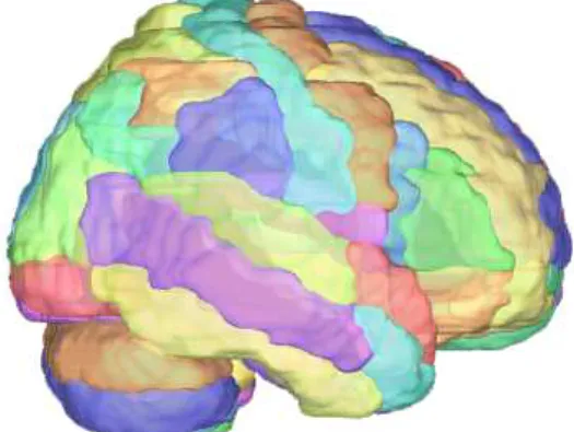
Contacts were grouped in discrete regions according to the Automated Anatomical Labeling (AAL) atlas[21]_{, which is divided as shown in ﬁgure 2.1. The standardized MNI coordinates of}

each multielectrode contact were determined by normalizing each individual MRI volume into MNI space, whereas the AAL atlas region was used to identify in which anatomical parcelation (area, region or site) the contact was placed. In our cohort (across diﬀerent patients, see Table 1, in Annex), multielectrode contacts were present in 62 of the 116 cerebral regions featured in the AAL atlas.

Figure 2.1: Regions comprising the AAL Atlas

Intracranial EEG signals recorded by contacts of the same patient which fell within the boundaries of the same AAL region were averaged across, yielding a single representative time series per region for each patient for each dataset (RS-iEEG and Stim-iEEG).

(33)

2.7 Mathematical methods for analysis

Diﬀerent mathematical approaches, considering the properties of iEEG time series, are available to compute functional and eﬀective brain connectivity maps[22–24]_{, and allow the compilation of}

the so-called adjacency matrixes between region pairs. The iEEG analyses methods employed in this study can be divided in three groups: time-based methods, information-based methods and frequency-based methods.

2.7.1 Time-based

Time-based methods are based on measuring the similarity of two different time-series as a function of a parameter called ‘time-lag’. Roughly speaking, they consist in comparing a given time series with the ‘past’ or the ‘future’ of a second time-series. Since iEEG time-series are non-linear, it is necessary to use specific analytic tools that fulfil and respect this condition. We used the nonlinear correlation coefficient, which is defined as the maximum of the following equation:

h2_xy(τxy) = PN

k=1y(k+τxy)2−PNk=1(y(k+τxy)−f(x(k)))2 PN

k=1y(k+τxy)2

(2.2)

where f is a nonlinear ﬁtting curve that approximates the statistical relationship between the signal x and y.

This measurement can be combined with the direction index[25]_{, which is computed with the}

nonlinear correlation coeﬃcients h2_xy and h2_yx and their time delaysτxy and τyx (as follows): D= 1

2(sgn(∆h

2_{) +}_sgn_(∆_τ₎₎ _(2.3)

To measure similarities on RS-iEEG activity from different regions,h2_xy was pair-wise mea-sured by using equation 2.2, computed using x and y as signals from different regions. These measurements, computed for each patient, allowed us to establish weighted adjacency matrixes for each patient (see fig. 2.2a) modelling the patient-based connectivity between the implanted regions. In order to determine which of these connections were meaningful, we thresholded each adjacency matrices using a density threshold that filtered out the weakest links between regions. The threshold value was based on a recently validated criterion[26] _{that maximizes the ratio}

between the overall efficiency of a network and its wiring cost. This criterion establishes that the average node degree (the number of edges connected to a node) has to be approximately 3, which leads to a total number of edges, m, in the connectome, that scales as m = (3/2)∗n, with nbeing the number of nodes. Following this relation, the weakest edges were filtered out, obtaining a binarized version of the adjacency matrix including only the significantly meaningful edges. Using equation 2.3, the directionality of the information was assessed.

(34)

Figure 2.2: (a) example of a weighted adjacency matrix for h2 values, in which every pair-wise edge has a value from 0 to 1. The diagonal of the matrix is set to 0, and represents the pair-wise edge between the pairs of the same region; (b) example of the adjacency matrix from the same dataset shown

in (a) after thresholding and binarization, where the only values left are the ones that represent a meaningful connection (and are all set to 1) and every other value is 0.

2.7.2 Information-based approaches: mutual information index

Another method to compare two iEEG signals consists in using information-based measures. These are based on the concept of Shannon entropy, which can be deﬁned as the expected value of the information contained in each signal. We deﬁne Shannon entropy as:

IX =X x

px(x)log 1 px(x)

(2.4)

Wherepx is the probability of character number x showing up in a stream of characters of the given "script". If we now consider two random variables X and Y, we can estimate their mutual dependence (mutual information), as the average amount of code necessary to encode the draws of a signal X using another signal Y, using the following equation:

M IXY =X xy

pXY(x, y)log pXY(x, y) px(x)py(y)

(2.5)

Although mutual information does not take into account potential asymmetries between pairs of iEEG time series, the analysis of resting-state data followed the same procedure reported for non-linear correlation coeﬃcient, h2

xy, reported in section 2.7.1. The same type of weighted adjacency matrixes was calculated, and the above-reported procedure to threshold them was employed (see ﬁg. 2.2). Moreover, since mutual information indexes do not permit estimations of directionality, the sense of direction (which node was the driver and which one the follower) in which information ﬂowed remained undetermined from these analyses.

2.7.3 Frequency-based Methods

In order to provide a causal or perturbation-based estimate of the functional strength linking the two brain regions, we also computed functional connectivity measures (and aimed to compile an atlas thereof) during episodic rhythmic entrainment with intracranial 50 Hz short electrical bursts (as compared to prior and following) between the region being stimulated and a sec-ond brain region (see our Stim-iEEG dataset). This type of functional signature was deﬁned

(35)

in our Stim-iEEG dataset as the enhancement of frequency speciﬁc local oscillatory activity, phase-locked (i.e., synchronized in phase) to individual pulses integrating the source of rhyth-mic electrical stimulation[2, 10]_{, during the 50 Hz burst delivery period. The enhancement of}

oscillatory activity was deﬁned by (1) an increase of 50 Hz power during the stimulation pe-riod, and (2) enhanced and sustained phase-coupling between the induced rhythmic activity and the output of the stimulation[10, 27]_{. We extracted time-frequency maps by convoluting each}

reference-free iEEG signal with a complex Morlet wavelet[28, 29]_:

W(t, f0) = (2πσt2)−

1 2e

−t 2

2σ2_t_e2iπf0t (2.6)

in which the relation f0

σf (whereσf =

1

2πσtwas set to 6.7[28]. These measures were computed

on frequencies from 1 to 100 Hz, in 1 Hz steps. As we were interested in measuring increases of power and/or phase coupling, we calculated the percent change compared to baseline [-300 to -100 ms], prior to burst onset in the 45-55 Hz frequency band. However, these measures do not reflect the extent to which electrically induced gamma oscillations are time-locked to the electrical pulses delivered by the intracranial electrical stimulator. The temporal dynamics of the instantaneous phase, between the electrical output delivered by the two stimulation contacts on each electrical burst and the 50 Hz-component of each of the iEEG time series recorded within the stimulating multielectrode, were computed for each time series. Only contacts showing average power increases in the [45-55 Hz] band during the stimulation period 10 times higher than the pre-stimulation onset baseline were considered. A modelled signal emulating the 50 Hz pattern delivered by the electrical stimulator was generated using an in-house script in Matlab (Mathworks, MA, USA). Artificially generated signals had the same length and sampling rate (1024 Hz) as the original data, with the value “+1” (followed by a “-1” to account for its biphasic waveform) taken at the onset of the electrical stimulation, and repeated every 20 ms for the duration of the stimulation epoch, whereas a value of “0” was added everywhere else along the time series. We calculated the instantaneous phase difference by comparing the modelled quadratic waveform emulating the 50 Hz burst delivered by the electrical stimulator with the gamma [45-55 Hz] iEEG components (post-artifact removal) recorded by each multielectrode contacts of the implantation scheme[2]_{. We computed for each pair of the above-described}

time-series (using the Morlet wavelet coeﬃcients of the modelled stimulator output signal and the iEEG recordings for each contact not involved in the stimulation) the phase diﬀerence, and estimated during 50 Hz stimulation the phase-synchrony, between these two signals. To that end, we applied the equation shown below:

e[i(ϕz(f,t)−ϕx(f,t))] = Wx(f, t)W ∗ x(f, t)

|Wx(f, t)||Wz(f, t)|

(2.7)

whereW represents the Morlet coeﬃcient for each frequencyf and timet;xand zare each of the two signals (iEEG and the stimulator) andphix and phiz their instantaneous phase[30].

To measure the consistency over time of the phase diﬀerence between these two signals, the single-trial phase-locking value (S-PLV)[31] _{described by the following equation, was calculated:}

SP LV =|1

δ

Z t+δ/2

t−δ/2

e[i(ϕz(f,τ)−ϕx(f,τ))]_dτ_| (2.8) wheredeltarepresents a time period covering a speciﬁc number of cycles within the frequency of interest. Following recommendations[30, 32]_{, it was used}_delta _{= 200 ms, which corresponded}

(36)

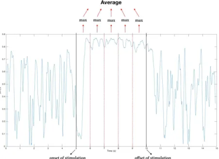
of phase-difference) to 1 (indicating the strongest phase-locking possible). To determine which S-PLV values would account for the two most relevant 5-second-long periods, i.e., baseline of 5 seconds prior to stimulation (pre-stimulation) and 5 seconds during stimulation (stimulation), each of these periods was divided into 5 x 1 second windows. The highest S-PLVs for each 1 second window were singled out and the 5 highest S-PLVs (one for each 1-second window of iEEG activity) were averaged across. The final average of such 5 highest mean S-PLV was taken as a representative estimate of the pre-stimulation and the stimulation 5 second periods. This approach, which is exemplified in fig. 2.3, was used to limit variability in the S-PLVs.

Figure 2.3: Method applied to determine mean S-PLV representative for the pre-stimulation or stimulation periods for Stim-iEEG datasets. Each 5 seconds’ long period (pre-stimulation and stimulation periods) were subdivided into 5 x 1 second periods in the highest S-PLV was singled out.

The highest S-PLV value of each 1 second windows were averaged through, yielding a representative estimate for the whole 5 second period.

Given our interest in measuring increases of S-PLV by comparing iEEG recordings obtained prior and during stimulation, pre-stimulation representative S-PLV estimates calculated as in-dicated above were used as baseline to normalize the representative S-PLVs for the stimulation period. Normalization was performed by subtracting the former from the latter (i.e., S-PLV during stimulation – S-PLV prior to stimulation)[33]

Similarly to what has been described in sections 2.7.1 and 2.7.2, we built an S-PLV connectiv-ity matrix, which included data from every patient of our cohort, for both low and high intensconnectiv-ity Stim-iEEG datasets. Considering data only from stimulation trials in which pairs of adjacent contacts delivering electrical current were both within the boundaries of the same AAL region (hence excluding time series in which this might not have been the case), the representative S-PLVs of diﬀerent patients associated to pairs of time series stimulated on and recorded from the same AAL region were averaged through, in order to end up with a ﬁnal single S-PLV value for each pair-wise edge probed with stimulation representing the cohort of studied patients. This procedure was conducted for every region in which stimulations bursts were delivered (n=42 stimulated/iEEG sampled regions). Since not every AAL region considered in the Stim-iEEG

(37)

dataset were stimulated, note that the number of regions of the stim-iEEG mapping was lower than those present in the RS-iEEG dataset (n=62 iEEG sampled regions).

Using the same thresholding approach and criteria mentioned previously (see sections 2.7.1 and 2.7.2) our weighted S-LPV matrix, of 43 regions, was binarized (1 vs. 0) via S-PLV values, by assigning a value of 1 only to the relevant connection edges and a value of 0 to the remaining ones that did not fulﬁl this condition. Directionality was assessed based on the assumption that information had to necessarily ﬂow from the region where the electrical stimulation was delivered towards any remaining AAL brain region or regions hosting at least a multielectrode contact.

To compile the group RS-iEEG functional connectivity maps comparable (in spite of obvious differences in the number of nodes and edges and the use of stimulation only in the Stim-iEEG dataset) to those obtained during gamma electrical stimulation, S-PLV calculations were also conducted for the RS-iEEG dataset using the same main procedure described for Stim-iEEG maps in the preceding paragraphs. Instantaneous phase differences between the gamma [45-55 Hz] iEEG components at rest were computed. Nonetheless, since, RS-iEEG datasets were recorded at rest in absence of stimulation bursts, we were unable to use the exact same above-mentioned metrics (and in particular to compare functional interactions between the pulses delivered by the stimulation bursts and iEEG activity from AAL regions hosting at least a recording contact). Instead 2-second iEEG signals estimated for all pairs of AAL regions were compared across. As previously done for Stim-iEEG datasets, the consistency over time of the phase difference (S-PLV) between each pair of time-series was again computed using the above-mentioned equation 2.8. In contrast with the procedure applied to Stim-iEEG dataset (for which the average of the 5 highest S-PLV extracted from 5x 1-second windows was taken as the representative S-PLV measures for each 5-second pre- and stimulation periods), for RS-iEEG data we estimated the representative S-PLV as the arithmetic mean of instantaneous SPLV across each complete 2-second-long RS-iEEG signals.

2.8 Brain Map construction

Individual and group functional connectivity maps (functional connectomes), for both resting-state (RS-iEEG) and stimulation – high and low – (STIM-iEEG) datasets, were constructed using NeuroMArVl (Monash University, Melbourne, Australia). This is a browser-based soft-ware to produce graphic renderings of brain connectomes. For such representations, the MNI coordinates attributed to each AAL regions from which data were included in the connectome (hence being a node of the graph) were estimated as the mean between the MNI x, y and z coordinates of the contacts whose iEEG or stimulation modelled signals had been averaged as representative for that region. Beneﬁtting from its ability to provide directionality information (i.e., which node of given interaction is likely to drive/or lead and which one follows), the binary matrices employed to represent functional connectivity maps for RS-iEEG dataset were based on the non-linear correlation coeﬃcient (h2

xy). Additionally, however, S-PLV based RS-iEEG connectivity maps were also computed to facilitate (in spite of the many diﬀerences between the two) a qualitative/quantitative comparison between connectomes compiled on the basis of the RS-iEEG and Stim-iEEG datasets. The functional connectomes based on Stim-iEEG dataset were only constructed using S-PLV datasets.

2.9 Topological properties of the networks

(38)

measure estimates the number of edges connected to a single node within a connectome. For an adjacency matrix A, the degree for a node indexed by I in an undirected network is deﬁned as:

ki = X

j

aij (2.9)

where the sum is calculated across each node within a given connectome.

In the case of a directed network, each node has two degrees, an out-degree and an in-degree. The ﬁrst is the number of outgoing edges emerging from a given node deﬁned as follows:

k_iout=X j

aji (2.10)

and the second is the number of incoming edges onto a node calculated by using the formula below:

k_iin=X j

aij (2.11)

The total degree of a node in a directed network is, then, the sum of its in-degree and out-degree:

ktot_i =kin_i +k_iout (2.12)

2.10 Statistical Analyses

Non-parametric Spearman rank tests were used to estimate the statistical signiﬁcance of the correlations between h2

xy and S-PLV in resting-state data (i); h2xy and S-PLV for both low and high intensity stimulations (ii); h2_xy and 50 Hz pre vs. during stimulation power increases for both low and high intensity electrical gamma (50 Hz) stimulation (iii); S-PLV in resting-state data and S-PLV for both low and high intensity electrical gamma stimulation (iv); S-PLV in resting-state data and Power for both low and high intensity electrical stimulation (v); S-PLV for both low and high intensity stimulation and 50 Hz power pre vs. during stimulation increases for both low and high intensity electrical gamma bursts (vi), S-PLV for low intensity electrical stimulation and SPLV diﬀerence for high intensity electrical stimulations (vii), and pre vs. during stimulation power increases for low intensity and also for high intensity electrical gamma bursts (viii). For all tests, signiﬁcance level was set at p < 0.05.

(39)

Chapter 3

Results

3.1 Stimulation iEEG-based connectome

To facilitate a better understanding of the complex and long series of analysis we performed, our results will ﬁrst be presented on a dataset of a representative patient (n=1, patient reference no. 1998), followed by the results for the whole population of epileptic patients (n=18) analysed for this dissertation.

3.1.1 Example of a single patient connectome

Patient reference number 1998 had multielectrode contacts implanted in the following 11 AAL regions of the right hemisphere and the cerebellum: Supramarginal Gyrus, Angular Gyrus, Inferior Parietal Lobule, Middle Occipital Gyrus, Superior Temporal Gyrus, Fusiform Gyrus, Inferior Temporal Gyrus, Middle Temporal Gyrus, Lobule III of Cerebellar Hemisphere, Crus I of Cerebellar Hemisphere and Inferior Occipital Cortex (number of contacts on each region and additional information are presented at the table annexed). Connections between regions were established pair-wise on the basis of our established criteria for enhanced neural entrainment. We considered regions that showed both increase of S-PLV and 50 Hz power at least 10 times higher than base-line pre-stimulation values (see methods section for details). As we divided electrical stimulation in two diﬀerent groups based on the intensity, two diﬀerent connectivity maps, one for high and one for low stimulation intensity, will be presented.

The High Intensity Stim-iEEG connectome of patient reference 1998 is represented in the