Do hedge fund indices enhance portfolio performance?

Texto

(1)MASTER OF SCIENCE IN FINANCE. MASTERS FINAL WORK DISSERTATION. DO HEDGE FUND INDICES ENHANCE PORTFOLIO PERFORMANCE?. GONÇALO MARIA OLIVEIRA DÁ MESQUITA LIBERAL. NOVEMBER - 2016.

(2) MASTER OF SCIENCE IN FINANCE. MASTERS FINAL WORK DISSERTATION. DO HEDGE FUND INDICES ENHANCE PORTFOLIO PERFORMANCE?. GONÇALO MARIA OLIVEIRA DÁ MESQUITA LIBERAL. SUPERVISOR: PROF. MARIA TERESA MEDEIROS GARCIA. NOVEMBER - 2016.

(3) Abstract Traditional investment portfolios are focused only on two asset classes: Stocks and Bonds. In recent decades institutional portfolios and private investors have, for balanced risk profiles, focused on 60% of global stock usually through the US S&P500 and 40% bonds through the Barclays US Aggregate Bond Index. These portfolios seek a passive exposure to a diversified portfolio on financial markets in order to obtain risk-adjusted returns for long-term investments. The component of bonds tends to lower the volatility of the stocks resulting in lower volatility of these portfolios. Given the current low interest rates and low bond yields, this asset class could increase its volatility, thus contributing to an increased risk of these portfolios. Therefore, it is necessary to increase exposure to other financial instruments in order to diversify these portfolios and reduce systemic risks in financial markets. If so, investors should consider adding alternatives to their traditional investments as a way to potentially reduce their portfolios sensitivity to financial markets. It is therefore necessary to consider investment alternatives, in order to get adjusted returns to risk in setting up investment portfolios. Absolute return funds or hedge funds, may present a valid alternative investment in times of high volatility, and have gained visibility in periods of bear markets compared. 1.

(4) to stock index funds, consequently leading to an increase in demand, i.e., an increase of assets under management for these assets. This study aims to analyze the combination of investable indices of hedge funds in a traditional portfolio of 60% stocks and 40% bonds. It is intended to determine the minimum variance portfolio and Markowitz and the respective weights of hedge fund indices in the reference portfolio and compare their performance considering time windows of two, five and ten years. This is designed to study the effect of integration of investable hedge fund indices and the effect of their inclusion in a diversified portfolio of stocks and bonds. Further on, we will perform the historical analysis of the optimal investment portfolio, taking into account the Markowitz model and minimum variance model and compare the most common performance parameters: Sharpe ratio, Treynor ratio and alpha Jensen with the portfolio benchmark.. Jel Classification: G11, G12 Keywords: Hedge Funds, Absolute Return, Sharpe Ratio, Global Equity-Bond portfolios, Markowitz Portfolio Theory, Minimum-variance Portfolio, Optimal Portfolios, Investable Hedge Fund Index, Performance Evaluation.. 2.

(5) Resumo As carteiras de investimento tradicionais são focadas apenas em duas classes de ativos: Ações e Obrigações. Nas últimas décadas as carteiras institucionais, e de investidores privados, para perfis de risco equilibrados têm colocado o foco em 60% de ações globais, usualmente através do índice americano S&P500, e em 40% de obrigações através do índice Barclays US Aggregate Bond. Estas carteiras procuram de uma forma passiva uma exposição a uma carteira diversificada aos mercados financeiros, com o objetivo de obter retornos ajustados ao risco para períodos de investimento de longo prazo. A componente de obrigações tende a baixar a volatilidade das ações, resultando numa menor volatilidade destas carteiras. Dadas as atuais baixas taxas de juros, e as baixas yields das obrigações, esta classe de ativos poderá aumentar a sua volatilidade contribuindo para um maior risco destas carteiras. Posto isto, poderá fazer sentido aumentar a exposição a outros instrumentos financeiros por forma a diversificar estas carteiras e diminuir os riscos sistemáticos dos mercados financeiros. Torna-se assim necessário considerar alternativas de investimento, com o objetivo de obter retornos ajustados ao risco na constituição de carteiras de investimento. Os fundos de investimento de retorno absoluto, ou hedge funds, podem constituir alternativas de investimento válidas em períodos de alta volatilidade, e têm ganho visibilidade em períodos de bear market face a fundos de índices de ações,. 3.

(6) consequentemente originando um aumento da procura, ou seja, a um aumento dos ativos sobre gestão. O presente trabalho tem como objetivo estudar a combinação de índices investíveis de Hedge Funds numa carteira tradicional de 60% de ações e 40% de obrigações. Pretende-se determinar a carteira de variância mínima e de Markowitz e os respetivos pesos dos índices de hedge funds na carteira de referência e comparar a sua performance considerando janelas temporais de dois, cinco e dez anos. Pretende-se assim apurar o efeito da integração de índices investíveis de hedge funds e o efeito da sua inclusão numa carteira diversificada de ações e obrigações. Será também observada a análise histórica da carteira ótima de investimento, tendo em conta o modelo de Markowitz e o modelo de variância mínima, bem como comparados os parâmetros de performance mais habituais: rácio de Sharpe, rácio de Treynor e alfa de Jensen com a carteira de referência.. Jel Classificação: G11, G12 Palavras-Chave: Fundos de Cobertura de Risco, Fundos de Retorno Absoluto, Rácio de Sharpe, Carteiras globais de ações e obrigações, Teoria da Carteira de Markowitz, Carteira de variância mínima, Carteiras óptimas, Índices de Hedge Funds Investíveis, Avaliação de performance.. 4.

(7) Acknowledgments. I dedicate this dissertation first and foremost to my mother, who was and always will be in my thoughts. I would like to express my sincere gratitude to my supervisor Prof. Teresa Garcia, who provided me with guidance, support and motivation whilst leaving me the freedom to explore the topics I was interested in. I would also like to thank all my teachers who provided me with the knowledge and tools required to complete my master’s dissertation. I would also like to thank my parents for all their support during my entire academic and professional career and especially thank to my girlfriend, Sofia Ferreira, for her support and extra patience over the last two years. Thank you for the sleepless nights and understanding of my absence in several occasions. Last but not least, to all my friends, especially André Ramos and Pedro Neves for all the moral support and encouragement they gave me to conclude my dissertation.. 5.

(8) CONTENTS 1.. Introduction................................................................................................................1 1.1. Introducing hedge funds allocation in a typical global equity-bond. portfolio .........................................................................................................................1 1.2 2.. 3.. Literature review ........................................................................................................4 2.1. Modern Portfolio Theory and the Optimal Portfolio ..........................................4. 2.2. The 60 / 40 stock and bond portfolio allocation ................................................6. 2.3. Hedge funds industry and absolute return strategies ........................................8. Methodology ............................................................................................................14 3.1. The benchmark index: 60/40 portfolio .............................................................14. 3.2. Selecting absolute return index ........................................................................15. 3.3. Determine the hedge fund allocation...............................................................18. 3.4. Measures of performance and basic concepts .................................................18. 3.4.1. Return ........................................................................................................19. 3.4.2. Simple return or Arithmetic Return (AR) ...................................................19. 3.4.3. Standard deviation ....................................................................................20. 3.4.4. Beta ............................................................................................................21. 3.5. 4.. Dissertation objectives .......................................................................................3. Performance measures .....................................................................................22. 3.5.1. Sharpe Ratio ..............................................................................................22. 3.5.2. Treynor Ratio .............................................................................................23. 3.5.3. Jensen’s Alpha ...........................................................................................23. 3.5.4. Information Ratio ......................................................................................24. Data analysis.............................................................................................................25. 6.

(9) 4.1. 4.1.1. The traditional equity-bond portfolio and hedge fund style index ...........25. 4.1.2. The minimum variance portfolio ...............................................................26. 4.1.3. The Markowitz portfolio ............................................................................28. 4.1.4. The efficient frontier and optimal portfolio ..............................................28. 4.2 5.. Assessing optimal absolute return allocation in the selected portfolio ...........25. Data analysis and calculations ..........................................................................29. Conclusions, limitations and further investigation topics .......................................35 5.1. Conclusion .........................................................................................................35. 5.2. Study limitations ...............................................................................................36. 5.3. Topics for further Investigation and recommendations...................................38. 6.. References ................................................................................................................39. 7.. Appendix ..................................................................................................................43. 7.

(10) LIST OF TABLES Table I – Performance and risk of the portfolio 60/40 between 2006 and 2016 .......... 26 Table II – Performance and risk of the hedge fund strategies between 2006 and 2016 ................................................................................................................................ 26 Table III – Risk and performance indicators for the portfolio 60/40 and portfolio A for ten, five and two year periods .................................................................................. 30 Table IV – Risk and performance indicators for the portfolio 60/40 and portfolio B for ten, five and two years period. ................................................................................. 32 Table V – Risk and performance indicators for the portfolio 60/40 and portfolio C for ten, five and two years period........................................................................................ 33. Table A.I - Increasing weight of HF1 - MEBI Maximum Sharpe Ratio Strategy L1 index into the 60/40 portfolio and the effect on volatility, expected return and Sharpe ratio into the overall portfolio ........................................................................................ 43 Table A.II - Increasing weight of HF2 - MEBI Zero Beta Strategy L1 index into the 60/40 Portfolio and the effect on volatility, expected return and Sharpe ratio into the overall Portfolio ........................................................................................................ 46 Table A.III - Increasing weight of HF3 - MEBI Eurekahedge ILS Advisers Index into the 60/40 Portfolio and the effect on volatility, expected return and Sharpe ratio into the overall Portfolio ........................................................................................................ 49. 8.

(11) LIST OF FIGURES Figure 1 – Markowitz efficient frontier. ............................................................................5 Figure 2 – Historical Growth of Assets under Management for the hedge fund industry, 1997 - 2016. ......................................................................................................11 Figure 3 – Historical evolution of Portfolio 60/40, S&P 500 and Barclays US Aggregate Bond, between 01-jan-2006 and 31-jan-2016. ..............................................15 Figure 4 – Venn diagram of the 5 major hedge funds databases, where is represented the percentage of funds covered by each database individually and by all possible combinations of multiple databases. ...........................................................16. Figure A.1 – Effect on Volatility and Average Annual Return of portfolio with increasing weight of HF1 into the traditional 60/40 portfolio during the ten year period...............................................................................................................................44 Figure A.2 – Effect on Volatility and Average Annual Return of portfolio with increasing weight of HF1 into the traditional 60/40 portfolio during the five year period...............................................................................................................................44 Figure A.3 – Sharpe Index of portfolio at different weightings of HF1 into the traditional 60/40 portfolio during the ten year period ...................................................45 Figure A.4 – Efficient Frontier combining HF1 with the traditional 60/40 portfolio during the ten year period ..............................................................................................45 Figure A.5 – Effect on Volatility and Average Annual Return of portfolio with increasing weight of HF2 into the traditional 60/40 portfolio during the ten year period...............................................................................................................................47. 9.

(12) Figure A.6 – Effect on Volatility and Average Annual Return of portfolio with increasing weight of HF2 into the traditional 60/40 portfolio during the five year period...............................................................................................................................47 Figure A.7 – Sharpe Index of portfolio at different weightings of HF2 into the traditional 60/40 portfolio during the ten year period ...................................................48 Figure A.8 – Efficient Frontier combining HF2 with the traditional 60/40 portfolio during the ten year period ..............................................................................................48 Figure A.9 – Effect on Volatility and Average Annual Return of portfolio with increasing weight of HF3 into the traditional 60/40 portfolio during the ten year period...............................................................................................................................50 Figure A.10 – Effect on Volatility and Average Annual Return of portfolio with increasing weight of HF3 into the traditional 60/40 portfolio during the five year period...............................................................................................................................50 Figure A.11 – Sharpe Index of portfolio at different weightings of HF3 into the traditional 60/40 portfolio during the ten year period ...................................................51 Figure A.12 – Efficient Frontier combining HF3 with the traditional 60/40 portfolio during the ten year period ..............................................................................................51 Figure A.13 – Evolution of 100.000 USD of static Portfolio 60/40 vs Portfolio A in 10 years ................................................................................................................................52 Figure A.14 – Evolution of 100.000 USD of static Portfolio 60/40 vs Portfolio B in 10 years ................................................................................................................................53 Figure A.15 – Growth of 100.000 USD of static Portfolio 60/40 vs Portfolio B in 10 years ................................................................................................................................54. 10.

(13) 1. Introduction 1.1 Introducing hedge funds allocation in a typical global equity-bond portfolio For many years, Institutional investors such as public and private pension funds, as well as sovereign funds and insurance companies have focused their asset allocation in typical portfolios composed of 60% equities and 40% bonds. For some private investors and balanced fund managers this is the ideal asset allocation for their longterm investments. With this approach, also known as the 60-40 equity/fixed income portfolio, investors tend to follow a combination of global stocks and global bonds and expect that with only two asset classes a simple and diversified portfolio is formed in order to achieve improved risk-adjusted performance. This approach is used by passive investors for long-term growth. It consists in combining only two Exchange-Traded Funds (ETFs), and by rebalancing it periodically and actively fund managers use this strategy as a benchmark in moderate or balanced mutual funds. These portfolios also have risk benefits, allowing for broader exposure to equities along with lower volatility provided by bonds than all equity portfolios. Bonds also provide diversification benefits with low correlation between bonds and stocks, which when combined in a portfolio results in a risk-adjusted return. This strategy is also to be used in all market conditions.. 1.

(14) Although these portfolios have performed well between the 1980s and 1990s, with the passage to the 21st century and the change in interest rates a series of bear markets and low interest rates have eroded the popularity of these portfolios. Over the last decade, and with the decrease of interest rates and the increasing correlation between stocks and bonds, the performance and popularity of the 60/40 portfolios has deteriorated. Nevertheless, this portfolio allocation continues to play an important role in finance to this day. The prime goal of most investors is to minimize risk whilst maximizing return and expect positive returns in all market conditions. However, this fact is not a reality even in a well-diversified portfolio or a typical equity-fixed income portfolio, albeit an introduction of an asset that is uncorrelated to the market could contribute to that goal. Another asset class that has grown in popularity are hedge funds and absolute return strategies that aim at better risk adjusted performances. The present study aims at introducing hedge fund strategies or absolute return strategies allocation with a simple 60-40 equity-fixed income portfolio, in order to measure their performance on the overall portfolio.. 2.

(15) 1.2 Dissertation objectives This study aims to compare the performance of a passive index portfolio of 60% global equity and 40% global fixed income with the allocation of hedge funds strategies or absolute returns strategies in the main portfolio. The objective is to show that the global performance of a current portfolio can be improved when combined with hedge funds, illustrating that an investable hedge fund index can be an easy way to protect a conservative or balanced portfolio and minimize its volatility, whilst increasing the return and decreasing exposure to the market. It will also be studied the successful and accessible absolute return strategies that have been consistently a risk-adjusted performance in different timeframes. Moreover, one of the main objectives will be to demonstrate that an open hedge fund strategy is accessible to every investor and intends to show that a hedge fund industry can improve a conventional portfolio performance by investing in a Hedge fund index. Finally, another aspect to address is to put in evidence that investing in hedge funds via indexes allows a systematic market exposure to hedge funds and absolute return techniques that could successfully generate risk-adjusted returns with diversification benefits and more transparency and regulation than by directly investing in a hedge fund.. 3.

(16) 2. Literature review 2.1. Modern Portfolio Theory and the Optimal Portfolio. The Modern Portfolio Theory (MPT) was introduced by Harry Markowitz (1952a) with his paper on Portfolio Selection, for which he was later awarded a Nobel Prize in economics. In his paper it was stated the importance of diversification and the effects of covariance of assets in the choice of the optimal portfolio. Before that, the Classic Portfolio Theory (CPT), characterized by managing risk and return only on the analysis of individual securities and by the purchase of good rated companies or underpriced stocks. Portfolio construction was made according to the maximization of the expected value of the assets selection in order to achieve the higher expected overall portfolio return. In practice, investors were only focusing on the return and risk of individual securities. Markowitz (1952a) became a pioneer with MPT, and mathematically proved that diversification among multiple securities and selecting securities with lower covariances worked by reducing portfolio volatility, or risk. According to this new model, investors should select their portfolios based upon the expected return and the variance of return of each asset and determine asset weights, resulting in an overall risk-reward of the portfolio, thus minimizing the risk given a certain rate of return. In other words, the investment strategy should be managed in a risk diversification perspective, meaning that, for each level of risk, there exists a combination of assets. 4.

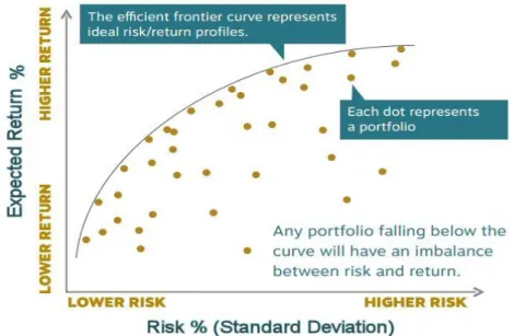
(17) that leads to at least the same return and a lower level of risk, which can be translated as our final objective in the search of the optimal portfolio. This leads to the representation of the efficient frontier, where each level of expected return, has the minimum level of volatility, or for a level of volatility has the higher expected return. This concept was introduced by Markowitz (1952a). The selection of the optimal portfolio should be made along the efficient frontier, and hoping to reach all investors profiles, Edwin & Gruber (2011). Investors always want to maximize the return to a determined level of risk or minimize the risk to a determined level of return and this relation should be represented across the efficient frontier, with a graphical representation curved, rather than linear, because of the benefit of diversification, as represented in Figure 1.. Figure 1 – Markowitz efficient frontier. Source: Diversification in a world of choices (https://www.bpvfunds.com/wpcontent/uploads/2015/02/DX-Bifold_Q4-2014.pdf). 5.

(18) Optimal portfolios that comprise the efficient frontier tend to have a higher degree of diversification than the sub-optimal ones, which are typically less diversified. An inefficient portfolio or sub-optimal portfolio lies below the efficient frontier because it does not provide enough return for the level of risk or does not have a higher level of risk for the defined rate of return, and therefore should not be selected by any rational investor which prefers an efficient portfolio, regardless of the investor profile. Bawa (1976) tested successfully Markowitz model for different investor profiles. The optimal portfolio selection is the efficient portfolio which maximizes the utility function of the investor, (Markowitz, b1952), i.e., with the greater expected utility in the investor perspective.. 2.2 The 60 / 40 stock and bond portfolio allocation The MPT focused on the construction of portfolios with two asset classes: Stocks and Bonds. In the 1950s these asset classes were used to build a well diversified portfolio. Markowitz (1952a) used the classical market-capitalization-weighted portfolio, whereas the 60/40 ratio of stocks and bonds represented the global universe of investable markets, and concluded that this combination provides the maximum return for a given amount of risk. This asset class blend has become the reference of a moderate or balanced portfolio over the last decades. Historically, this portfolio. 6.

(19) allocation has been shown to offer solid returns with a moderate risk profile over the long-term. Bernstein (2002). Implicit to this strategy besides the diversification is the uncorrelation of bonds and stocks. These two asset classes when combined and moving differently can smooth out volatility, resulting in a diversified portfolio that should be less volatile and the losses less severe than in an all equity portfolio. The overall risk and return of the 60/40 portfolio varies greatly and the volatility and risk premium of equities has changed ever since Markowitz presented his theory. The 60/40 portfolio in today’s market has more risk than the same allocation portfolio decades before. The correlation between stocks and bonds is increasing and low interest rates are associated with low bond yields and increasing volatility in bonds, as showed in the two-factor model by Fong and Vasicek (1991). When interest rates rise, bond prices tend to fall, according to Martellini et al. (2003) and the downside protection from bonds allocation will fail in periods with high volatility in stock market, as stated by Schwert (1989). The equity market fall of 40% in 2008 challenged the efficacy of the 60/40 model and proved that this portfolio was not properly diversified. Today’s investors and fund managers desire a smoother ride and better downside protection. For that purpose investors or institutional portfolios search for tools to customize portfolios and improve their performance in terms of risk-adjusted returns, volatility, diversification, correlation and downside protection.. 7.

(20) The 60/40 model is limited to stocks and bonds because those were the only asset classes available to most investors at the time when the MPT gain popularity, but in today’s market investors who want to beat their performance combine other investment vehicles, including currency, commodities, derivatives contracts, absolute return funds, managed futures, real estate, and even collectibles. The scope of this work is to study hedge funds or absolute return indexes allocation in the 60/40 portfolio. 2.3 Hedge funds industry and absolute return strategies The term hedge fund is commonly used to describe an alternative investment with the goal of generating improved risk-adjusted performance or absolute returns. Many hedge funds are not actually hedged and they often take large risks on speculative strategies to make performance returns irrespective of which way the markets are going. According to Anson (2006), the term “hedge fund" was first applied in 1949 by Alfred Jones to his private investment fund, which combined the simultaneous use of long and short equity positions to "hedge" the portfolio's exposure to movements in the market, as stated by Purcell et al. (1999). This strategy is known as Long Short Equity and is the most common used in hedge funds today. McCrary (2005). Nowadays, hedge funds often do not really "hedge" market risk and his definition is not precise. For Ackermann (1999), hedge funds began as investment partnerships that. 8.

(21) could take long and short positions. However, they have evolved into a multifaceted organizational structure that defies simple definition. Hence, the author characterizes hedge funds by a set of features, namely a largely unregulated organizational structure, flexible investment strategies, relatively sophisticated investors, substantial managerial investment, and strong managerial incentives. Hedge funds may therefore yield insight into the impact of regulation, alternative investment practices, and incentive alignment on performance. This vision describes the structural shape of these investment vehicles, leading another author, Jaeger (2003) to state a simple definition, ”A hedge fund is an actively managed investment fund that seeks attractive absolute return. In pursuit of their absolute return objective, hedge funds use a wide variety of investment strategies and tools.” Today, the Hedge Fund Marketing Association has a simple definition, “A hedge fund is an alternative investment that is designed to protect investment portfolios from market uncertainty, while generating positive returns in both up and down markets. Throughout time investors have looked for ways to maximize profits while minimizing risk. The issue of shielding an investment from market risk is attempted (although not always successful) with alternative investments that try to mitigate loss and preserve capital. “. 9.

(22) The idea of a defensive instrument, designed to protect portfolios is present and will be used later in this work. Since hedge funds often have high minimum investments, these instruments are only accessible to institutional investors and very wealthy private investors or billionaires who can afford them. However, some Mutual Funds and UCITS1 are exclusive at investing in absolute return strategies with low minimum investments which are accessible to all types of investors. Although this type of financial instruments are considered complex, they have grown in popularity, resulting in an increasing trend up of assets under management (AUM) up until the present day. Figure 2 shows the increasing AUM for the hedge funds industry between 1997 and 2016.. 1. “UCITS” or “undertakings for the collective investment in transferable securities” are investment funds regulated at European Union level. They account for around 75% of all collective investments by small investors in Europe. The legislative instrument covering these funds is Directive 2014/91/EU. Source: European Commission Website.. 10.

(23) Figure 2 – Historical Growth of Assets under Management for the hedge fund industry, 1997 - 2016. Source: http://www.barclayhedge.com/ Hedge funds can be open or closed funds, and their managers can invest in a diverse range of markets employing a wide variety of financial instruments2 and risk management techniques, which can be divided into investment strategies.. The most common hedge fund investment strategies are divided into relative value and directional. According to Ackermann (1999) and Credit Suisse Hedge Fund Index rules, the component investment strategies that comprise the eleven style-based sectors are based on the following hedge fund investment strategies: Convertible Arbitrage: funds aim to profit from the purchase of convertible securities and the subsequent shorting of the underlying stock when there is a pricing discrepancy made in the conversion factor of the security.. 2. Long and short positions in securities, leverage, options, swaps, future contracts, and other derivatives.. 11.

(24) Fixed Income Arbitrage: generate profits by exploiting inefficiencies and price anomalies between related fixed income securities. This strategy may include leveraging long and short positions in fixed income securities and trading techniques involving interest rate swaps, government securities and futures; Dedicated Short Bias: funds take shorter than long positions and earn returns by maintaining net short exposure in long and short equities. Equity Market Neutral: the manager takes both long and short positions in stocks while attempts to lock-out or neutralize market risk. (i.e., a beta of zero is desired). Managers often apply leverage to enhance returns. Event Driven: the manager invests in various asset classes and seeks to profit from potential mispricing of securities related to a specific corporate or market event 3. These funds can invest in equities, fixed income instruments (investment grade, high yield, bank debt, convertible debt and distressed), options and various other derivatives. The common subcategories in Event Driven strategies are Risk Arbitrage and Distressed Securities. Risk Arbitrage: the manager attempts to capture the spreads in merger or acquisition transactions involving public companies after the terms of the transaction have been announced. Risk arbitrager typically buys the stock of the company being acquired and simultaneously shorts the acquirer’s stock according to the merger ratio. The principal risk is deal risk, should the deal fail to close. Distressed. Securities:. the. manager. focuses. on. companies. subject. to. financial/operational distress or bankruptcy proceedings. Such securities trade at 3. Mergers, bankruptcies, financial or operational stress, restructurings, asset sales, recapitalizations, spin-offs, litigation, regulatory and legislative changes as well as other types of corporate events.. 12.

(25) substantial discounts to intrinsic value due to difficulties in assessing their proper value. This strategy is generally long-biased in nature when the manager attempts to profit from the issuer’s ability to improve its operation, but may take short positions, and when is expected the success of the bankruptcy process, which ultimately leads to an exit strategy. Global Macro: managers carry long and short positions in the global markets. Their positions reflect their views on overall market directions as influenced by economic trends, events or changes in interest rates. Their fund Portfolios can include stocks, bonds, currencies, commodities and derivatives instruments. Managers also use leverage and most funds invest globally in developed and emerging markets. Profits are made by correctly anticipating price movements in global markets and having the flexibility to manage their portfolio instruments. Long/Short Equity: funds invest on both long and short sides of equity markets, generally focusing on diversifying or hedging across particular sectors, regions or market capitalizations. The use of leverage is common in their portfolios. Managed Futures or Commodity Trading Advisors (CTA): focus on investing in listed financial and commodity futures markets and currency markets around the world. Managers tend to employ systematic trading programs that largely rely upon historical price data and market trends. A significant amount of leverage is employed since the strategy involves the use of futures contracts. Multi-Strategy: managers allocate capital based on perceived opportunities among several hedge fund strategies. Through the diversification of capital, managers seek to deliver consistently positive returns regardless of the directional movement of. 13.

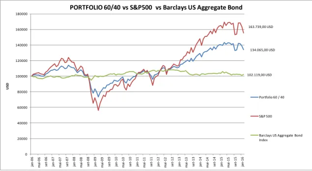
(26) markets. The added diversification benefits reduce the risk profile and help smooth returns, reduce volatility and decrease asset-class and single-strategy risks.. 3. Methodology 3.1 The benchmark index: 60/40 portfolio The conventional 60% equity 40% bond portfolio represents a moderate benchmark of this study. The 60/40 portfolio represents a passively managed index portfolio consisting of 60 percent on S&P 500 index 4and 40 percent on Barclays US Aggregate Bond Index5.. The historical data of S&P 500 index and Barclays US Aggregate Bond was taken from Datastream platform, from the 1st January 2006 to the 1st February 2016. Monthly data was used since it was the timeframe available for the hedge fund strategies. There is no theoretic unanimity concerning what the optimal performance period should be. However, many studies use 10 year periods. Therefore, we adopted a ten and five year periods to conduct our analysis. We focused on static portfolios, with no rebalancing (weights do not change between traditional equity bond portfolio). In Figure 3 we can observe the historical evolution of. 4. The Standard & Poor's 500 Index is a capitalization-weighted index of 500 stocks. The index is designed to measure performance of the broad domestic economy through changes in the aggregate market value of 500 stocks representing all major industries. 5 The index measures the performance of the U.S. investment grade bond market. The index invests in a wide spectrum of public, investment-grade, taxable, fixed income securities in the United States – including government, corporate, and international dollar-denominated bonds, as well as mortgage-backed and asset-backed securities, all with maturities of more than 1 year. Source: http://etfdb.com/. 14.

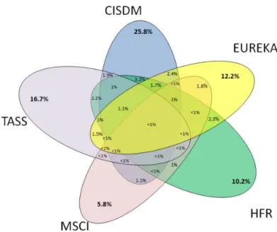
(27) traditional investment in the portfolio between the referred periods, where the yy axis represents the amount invested (An initial investment of $100,000 in January 2006). PORTFOLIO 60/40 vs S&P500 vs Barclays US Aggregate Bond 180000 163.739,00 USD. 160000. 140000. 134.065,00 USD 120000. 102.119,00 USD. USD. 100000. 80000. Portfolio 60 / 40 60000 S&P 500 40000 Barclays US Aggregate Bond Index. 20000. set-15. jan-16. mai-15. set-14. jan-15. mai-14. set-13. jan-14. mai-13. set-12. jan-13. mai-12. set-11. jan-12. mai-11. set-10. jan-11. mai-10. set-09. jan-10. mai-09. set-08. jan-09. mai-08. set-07. jan-08. mai-07. set-06. jan-07. jan-06. mai-06. 0. Figure 3 – Historical evolution of Portfolio 60/40, S&P 500 and Barclays US Aggregate Bond, between 01-jan-2006 and 31-jan-2016. Data assessed by the author of dissertation.. 3.2 Selecting absolute return index The hedge fund databases do not cover the whole hedge fund industry. Therefore, the hedge fund indices are not representative of the hedge fund universe (Agarwal et al, 2013). The five major hedge fund databases are: CISDM, HFR, Eureka, MSCI, and TASS. They represent the most comprehensive hedge funds database that has been used in the literature. According to Agarwal et al. (2013) less than one percent of the hedge fund industry reports to the databases referred above in 2009, as represented in the figure below:. 15.

(28) Figure 4 – Venn diagram of the 5 major hedge funds databases, where is represented the percentage of funds covered by each database individually and by all possible combinations of multiple databases. Source: Agarwal et al. (2013). The hedge fund database provider aggregates several funds that have reported performance and constructs indices itself. The hedge fund indices can be strategy specific, asset weighted, equally weighted, investable, or non-investable. In order to represent the hedge fund universe and to overcome the performance biases stated by Brown (1999), Fung and Hsieh (2000), we only used investable hedge fund indices. Therefore, investable indices are unaffected by survivorship or backfilling biases, according to Heidorn et al. (2010) and Park (1999). The term ‘investable’ means that the constituents of the index are open to investment, and not necessarily investing in the main index. This means that we cannot directly invest in the indices themselves. Investing in a hedge fund index is achieved via proxy. 16.

(29) products known as trackers that replicate an index performance. We selected a hedge fund database with investable indexes in which the investment is available by a tracker. For hedge fund indices we used data from the website www.eurekahedge.com. To select the eligible indices we used the two following requirements: 1) historical data from the last 10 years, from the first month of 2006 to the first month of 2016; and 2) an Index composed by liquid investable hedge funds, tracked by an investable fund that replicates index performance. Therefore, the three selected hedge fund indices were: . MEBI Maximum Sharpe Ratio L1. . MEBI Zero Beta Strategy L1. . Eurekahedge ILS Advisers Index. The MEBI Maximum Sharpe Ratio L1 is a Mizuho-Eurekahedge Bespoke index that aims to maximize the expected Sharpe ratio under pre-determined assumptions, with its 4 constituent assets: Japanese bonds, US bonds, Japanese equities and US equities. The index is updated on a daily basis on business days in Tokyo and Singapore. The MEBI Zero Beta Strategy L1 is a Mizuho-Eurekahedge Bespoke index that aims to have zero correlation on Japanese bonds under pre-determined assumptions, with its 4 constituent assets: Japanese bonds, US bonds, Japanese equities and US equities. The index is updated on a daily basis on business days in Tokyo and Singapore. The Eurekahedge ILS Advisers Index is ILS Advisers and Eurekahedge’s collaborative equally weighted index of 32 constituent funds. The index is designed to provide a broad measure of the performance of underlying hedge fund managers who explicitly allocate to insurance linked investments and have at least 70% of their portfolio invested in non-life risk. The index is base weighted at 100 at December 2005, does not contain duplicate funds and is denominated in local currencies. Source: www.eurekahedge.com. Each hedge fund will be denominated as HF1, HF2 and HF3, by the order above.. 17.

(30) 3.3 Determine the hedge fund allocation In order to assess the hedge fund allocation in the optimal portfolio, we compared two of the most common portfolio construction approaches: the minimum variance and the Markowitz portfolio. The minimum variance portfolio is the combination of risky assets that has the lowest possible variance, i.e., it is the efficient portfolio with lower risk, Bodie et al. (2011). The Markowitz portfolio is the combination of assets that maximizes the relation risk and return, i.e., the maximization of Sharpe ratio (1966). Short selling (or short positions) was restricted since it is not accessible for investors and, according to Elton et al. (2010), most institutional investors do not short sell, given that the practice is forbidden by law in many institutions. 3.4 Measures of performance and basic concepts After collecting data, we used MS Excel to compute data returns, standard deviation and covariance and then the measures of performance: Sharpe Ratio, Treynor Ratio, Jensen’s Alpha and Information Ratio. These measures of risk and performance were assessed for the benchmark portfolio and for the optimal portfolio. We expect the benchmark portfolio to be lowly correlated with the hedge fund strategy. Hence, it is expected that the variability of the overall portfolio or optimal portfolio decreases and the performance measures increases.. 18.

(31) The main concepts used to get these results are presented in the following items:. 3.4.1 Return To compute the returns, we used the following formula:. Where: is the logarithmic return of the asset i, at moment t; is the asset price in the moment t; is the asset price in the moment t-1;. In this work t represents a one month period. 3.4.2 Simple return or Arithmetic Return (AR) To calculate the absolute return in a period of time, we used the arithmetic return or simple return for the respective period, as follows:. Where: is the return of the asset i, at moment t; is the asset price in the moment t; is the asset price in the moment t-1;. 19.

(32) For the returns calculated over n successive time periods r1, r2, and rn, the cumulative return or overall return over the overall time period is:. Because there is no distribution of dividends, reinvestment of gains and losses, the appropriate average rate of return is the geometric average rate of return over n periods, which is:. Each return has an equal weight in the geometric average. For this reason, the geometric average is referred to as a time-weighted average.. Therefore, the geometric average return is equivalent to the annualized cumulative return over all n periods:. 3.4.3 Standard deviation The standard deviation of the returns was estimated from the historical data for daily or monthly returns. Afterwards, and in order to assess the annualized standard deviation, the following formula was used:. To obtain an accurate estimation of the volatility, in light of the intrinsic asymmetrical nature of return distributions proposed by Kaplan (2012), we computed the monthly. 20.

(33) logarithmic returns to estimate the monthly volatility and then multiplied it by the square root of 12, to get the annualized volatility of returns or the annualized standard deviation. 3.4.4 Beta Beta is a risk indicator that measures a security’s sensitivity to the index. It measures an asset's risk in relation to the market. A positive beta value indicates that assets generally move in the same direction with that of the market and vice versa. Elton and Gruber (1995) suggest that there is evidence that historical betas provide useful information about future betas. The formula for β is given by Sharpe (1964) in the Capital Asset Pricing Model:. Where, is the covariance between asset i with the market (or benchmark) is the market variance (or benchmark). Interpretations of beta: β<0: asset movement is in the opposite direction of the benchmark; β=0: asset movement is uncorrelated to the benchmark, which is the objective of absolute return strategies; 0<β>1: asset moves in the same direction, but in a lesser amount than the benchmark;. 21.

(34) β=1: asset moves in the same direction and in the same amount as the benchmark; β>1: asset moves in the same direction, but in a greater amount than the benchmark.. 3.5 Performance measures 3.5.1 Sharpe Ratio The Sharpe Ratio is a measure for calculating risk-adjusted return, which divides average portfolio excess returns over the sample period by the standard deviation of returns over that period. This measure was first referred by Sharpe (1966). It can be measured by:. SR =. Where, is the expected return of the portfolio; is the risk free rate;. is the portfolio standard deviation.. Investors also prefer portfolios with higher shape ratios (Sharpe, 1966), and the indicator for any portfolio will vary systematically with the assumed investment holding period (Bodie et al., 2011).. 22.

(35) 3.5.2 Treynor Ratio The Treynor Ratio is a measurement of portfolio excess returns, per each unit of the systematic risk, as follows:. T=. Where, is the expected return of the portfolio;. is the risk free rate;. is the Beta of the portfolio.. This measure was developed by Treynor (1966). The higher the Treynor ratio, the better the performance of the portfolio under analysis. This ratio is recommended for evaluating well diversified portfolios, and according to Treynor the ratio gives the excess returns that could have been earned on an investment that has no diversifiable risk. Later Treynor and Black (1973) reinforce the idea that risk in the specific security is significant to the investor only as it affects portfolio risk. 3.5.3 Jensen’s Alpha Jensen’s Alpha measures the average excess return on the portfolio in relation to the one predicted by the CAPM, for a given portfolio’s beta and the average market return. This indicator was originally designed to evaluate fund managers, Jensen (1968). A positive Alpha means that a portfolio outperformed the market, whilst a negative. 23.

(36) value indicates underperformance. The following formula was used to calculate the Alpha:. where, is the average return for portfolio p during a period of time;. is a measure of systematic risk for portfolio p;. is the average return on the market in period t; the risk-free rate of return during the period;. The higher the alpha, the more a portfolio has earned above the level predicted.. 3.5.4 Information Ratio The information ratio divides the alpha of the portfolio by the tracking error. It measures the excess return per unit of nonsystematic risk of the portfolio, or the risk that could be diversified away by holding a market index portfolio. The Information ratio (IR) is used for measuring active managers against a passive benchmark. This parameter is often used to evaluate mutual funds and hedge funds, since the IR shows the consistency of the fund manager in generating superior risk adjusted performance. A higher IR shows that the manager has outperformed other. 24.

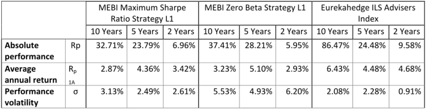
(37) fund managers and has delivered consistent returns over a specified period of time, Goodwin (1998). It can be measured by:. Where, is the Jensen’s Alpha;. , also denominated as tracking error, is the standard deviation of the difference between the returns of the portfolio and its benchmark.. 4. Data analysis 4.1 Assessing optimal absolute return allocation in the selected portfolio 4.1.1 The traditional equity-bond portfolio and hedge fund style index We assessed the absolute performance, the average annual return and the portfolio volatility for the traditional equity-bond portfolio for each hedge fund index. The following analysis refers to an investment over a 10 year period. Data was assessed for three different time periods: 10 years, 5 years and 2 years. In Table I we can observe the results for the traditional investment in global equity and global bonds and in Table II the individual results for each hedge fund strategy in the same period.. 25.

(38) Table I – Performance and risk of the portfolio 60/40 between 2006 and 2016 Portfolio 60 / 40 10 Years. 5 Years. 2 Years. Absolute performance. Rp. 38.70%. 35.36%. 7.24%. Average annual return. Rp 1A. 3.33%. 6.24%. 3.56%. 10.39%. 8.51%. 9.01%. Portfolio volatility. Table II – Performance and risk of the hedge fund strategies between 2006 and 2016 MEBI Maximum Sharpe MEBI Zero Beta Strategy L1 Ratio Strategy L1 10 Years 5 Years 2 Years 10 Years 5 Years 2 Years Absolute performance Average annual return Performance volatility. Rp Rp. 32.71% 23.79%. 6.96%. 37.41% 28.21%. 5.95%. Eurekahedge ILS Advisers Index 10 Years 5 Years 2 Years 86.47% 24.48%. 9.58%. 2.87%. 4.36%. 3.42%. 3.23%. 5.10%. 2.93%. 6.43%. 4.48%. 4.68%. 3.13%. 2.49%. 2.61%. 5.53%. 4.93%. 6.20%. 2.08%. 2.28%. 0.91%. 1A. 4.1.2 The minimum variance portfolio The following analysis refers to an investment in the traditional 60/40 portfolio and in each hedge fund index between January 2006 and February 2016. It is the purpose of the analysis to assess the minimum variance portfolio and observe how hedge funds indices reduce the variability or volatility of portfolio returns during the ten year period. We started to increase the weight of each hedge fund index in the traditional 60/40 equity-bond portfolio in order to assess the volatility of the combined portfolio. Three hedge fund style indices were used to assess the minimum variance portfolio. In Table A.I, Table A.II and Table A.III of the Appendix, we can observe the results for investments combinations of the traditional 60/40 equity bond portfolio and the MEBI. 26.

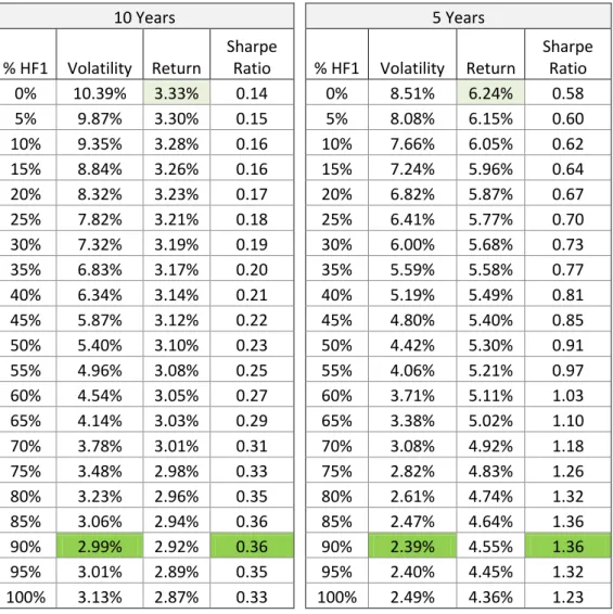
(39) Maximum Sharpe Ratio Strategy L1, MEBI Zero Beta Strategy L1 and Eurekahedge ILS Advisers Index (weightings from 0% to 100%). As showed in Table A.I and in Figure A.1, with an increasing allocation in the MEBI Maximum Sharpe Ratio Strategy L1 in the traditional 60/40 portfolio, the annual variability decreases. The optimal combination of this strategy is 91% of HF1 for the 10 year period, hence the traditional 60/40 portfolio annual volatility decreases from 10.32% to 2.99%. For a five year period, the ideal combination is 92%, as shown in Figure A.1, which illustrates the consistent optimal allocation for this hedge fund strategy. For the MEBI Zero Beta Strategy L1 we can observe in Figure A.5 that the optimal allocation, for the ten year period, is 78% and, for the five year period, is 75%, as represented in the Figure A.6. Regarding the third strategy, Eurekahedge ILS Advisers Index, the optimal allocation is obtained with a higher weight of 96% for the ten year period and of 93% for the five year period. The volatility of the overall portfolio decreases with the increasing allocation of this strategy, as we can observe in Figure A.9 for the ten year period and in Figure A.10 in the five year period.. 27.

(40) 4.1.3 The Markowitz portfolio For the Markowitz portfolio we used the same time period as the minimal variance portfolio. We started to increase the weight of each hedge fund index in the traditional 60/40 equity-bond portfolio and assessed the sharpe ratio of the combined portfolio. As we can observe in Figure A.3, when combining HF1 with the traditional equity-bond portfolio, there is a significant increase of the sharpe ratio of the overall portfolio. The maximum sharpe ratio has been found with a weight of 88% of HF1 considering the ten year period. In Figure A.7 for HF2 the optimal weight is 77%, considering the ten year period, and for HF3 the optimal weight is 99%, also for the same period, as we can observe in Figure A.11. As would be expected, the minimum variance portfolio that we have assessed before shows the best risk-return profile for each portfolio, and thus the hedge fund allocation strategy is similar between the minimum variance and the Markowitz portfolio. 4.1.4 The efficient frontier and optimal portfolio There is no significant difference in portfolio variance and Sharpe Ratio regarding the ideal hedge fund weights assessed before. Therefore, we can round up and assume that for each strategy the optimal hedge fund weight is: Portfolio A: 90% for HF1 and 10% 60/40 Portfolio; Portfolio B: 75% for HF2 and 25% 60/40 Portfolio;. 28.

(41) Portfolio C: 95% for HF3 and 5% 60/40 Portfolio.. For each hedge fund index, those are the portfolios that meet all investor’s profiles expecting to achieve the minimum variance whilst at the same time obtaining the best risk adjusted return. Henceforth, the optimal portfolios will be referred to as Portfolio A, Portfolio B and Portfolio C, for the combinations of HF1, HF2 and HF3, respectively, with the traditional 60/40 portfolio. We can also represent the efficient frontier for each hedge fund combination with the traditional equity-bond, where each level of expected return has the minimum level of volatility. We can observe the graphical representations of the efficient frontier inFigure A.4, Figure A.8 and Figure A.12, referring to HF1, HF2 and HF3, respectively.. 4.2 Data analysis and calculations We performed a backtest with the optimal hedge fund allocation previously presented for each strategy and assessed the performance measures for each portfolio. We considered the period between January 2006 and February 2016, referring to the ten, five and two last year’s periods. We then compared our three portfolios (A, B and C) with the benchmark portfolio, the 60/40 global equity-bond portfolio, for the same periods.. 29.

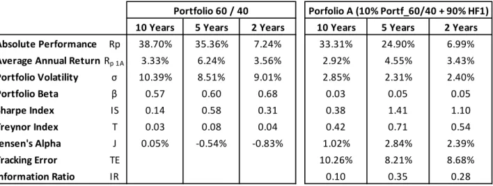
(42) For Portfolio A, when considering an investment of 90% weight in the MEBI Maximum Sharpe Ratio Strategy L1 index and 10% weight of the traditional Portfolio 60/40, we have assessed the risk and performance indicators, presented in Table III.. Table III – Risk and performance indicators for the portfolio 60/40 and portfolio A for ten, five and two year periods Portfolio 60 / 40. Porfolio A (10% Portf_60/40 + 90% HF1). 10 Years. 5 Years. 2 Years. 10 Years. 5 Years. 2 Years. 38.70%. 35.36%. 7.24%. 33.31%. 24.90%. 6.99%. Average Annual Return Rp 1A. 3.33%. 6.24%. 3.56%. 2.92%. 4.55%. 3.43%. Portfolio Volatility. 10.39%. 8.51%. 9.01%. 2.85%. 2.31%. 2.40%. Absolute Performance. Rp. Portfolio Beta. β. 0.57. 0.60. 0.68. 0.03. 0.05. 0.05. Sharpe Index. IS. 0.14. 0.58. 0.31. 0.38. 1.41. 1.10. Treynor Index. T. 0.03. 0.08. 0.04. 0.42. 0.71. 0.54. Jensen's Alpha. J. 0.05%. -0.54%. -0.83%. 1.02%. 2.84%. 2.39%. Tracking Error. TE. 10.26%. 8.21%. 8.68%. Information Ratio. IR. 0.10. 0.35. 0.28. The average annual return decreases slightly in the three different periods and the portfolio volatility significantly decreased from 10.39% to 2.85% in the ten year period and from 8.51% to 2.31% in the five year period. For the two year period, we obtained the same order of magnitude, that is, a decrease from 9.01% to 2.40% in the variability of the portfolio, resulting in a lower risk of the portfolio. Consequently, the Sharpe ratio of the portfolio increases with every time period in analysis, meaning that the portfolio achieved better risk adjusted returns.. 30.

(43) The portfolio beta decreases from 0.57 to 0.03 in the ten year period, reflecting a very low risk exposure or sensitivity to the market. For the five and two year periods, the portfolio beta was consistent with the ten year period. The Treynor ratio significantly increases in all time periods, which indicates a better performance of the portfolio under study. Jensen Alpha was positive, thus reflecting that the portfolio performed better when compared to its benchmark during the three time periods in analysis. The tracking error was higher, meaning that there are significant differences between the returns of the portfolio and its benchmark. The high Information Ratio shows that the portfolio has outperformed its benchmark and has delivered consistent returns over the period of time in analysis. In Figure A.13 we can observe the evolution of 100.000 USD under the static portfolio 60/40 vs portfolio A in 10 years.. For Portfolio B, when considering an investment of 75% weight in the MEBI MEBI Zero Beta Strategy L1 index and 25% weight of the traditional portfolio 60/40, we have assessed the risk and performance indicators, as presented in Table IV.. 31.

(44) Table IV – Risk and performance indicators for the portfolio 60/40 and portfolio B for ten, five and two years period. Portfolio 60 / 40. Porfolio B (25% Portf60/40 + 75% HF2). 10 Years. 5 Years. 2 Years. 10 Years. 5 Years. 2 Years. 38.70%. 35.36%. 7.24%. 37.73%. 29.94%. 6.28%. Average Annual Return Rp 1A. 3.33%. 6.24%. 3.56%. 3.25%. 5.38%. 3.09%. Portfolio Volatility. 10.39%. 8.51%. 9.01%. 4.66%. 4.22%. 5.25%. Absolute Performance. Rp. Portfolio Beta. β. 0.57. 0.60. 0.68. 0.10. 0.14. 0.18. Sharpe Index. IS. 0.14. 0.58. 0.31. 0.31. 0.97. 0.44. Treynor Index. T. 0.03. 0.08. 0.04. 0.14. 0.29. 0.13. Jensen's Alpha. J. 0.05%. -0.54%. -0.83%. 1.16%. 2.81%. 1.37%. Tracking Error. TE. 9.37%. 7.50%. 8.09%. Information Ratio. IR. 0.12. 0.37. 0.17. The average annual return decreases slightly in all time periods and the portfolio volatility significantly decreased from 10.39% to 4.66% in the ten year period, from 8.51% to 4.22 % in the five year period and from 9.01% to 5.25% in the two year period, thus resulting in a lower risk of the portfolio. Consequently, the Sharpe ratio of the portfolio increases in every time period in analysis, which means that this portfolio achieved better risk adjusted returns. The portfolio beta decreases from 0.57 to 0.10 in the ten year period, reflecting a very low risk exposure or sensitivity to the market. For the five and two year periods the portfolio beta was consistent with the ten year period. The Treynor ratio significantly increases in all time periods, indicating a better performance of the portfolio under study. Jensen Alpha was positive, thus showing that the portfolio performed better when compared to its benchmark during the three time periods of analysis.. 32.

(45) The tracking error is considerably high, meaning that returns of the portfolio differ from returns of its benchmark. The high Information Ratio shows that the portfolio has outperformed its benchmark and has delivered consistent returns over the period of time in analysis. In Figure A.14 we can observe the evolution of 100.000 USD under the static portfolio 60/40 vs portfolio B in 10 years.. Finally, for Portfolio C, with an investment of 95% weight in the Eurekahedge ILS Advisers Index and 5% weight of the traditional portfolio 60/40, the risk and performance indicators are presented in table V, below.. Table V – Risk and performance indicators for the portfolio 60/40 and portfolio C for ten, five and two years period. Portfolio 60 / 40 Absolute Performance. Rp. Porfolio C (5% Portf_60/40 + 95% HF3). 10 Years. 5 Years. 2 Years. 10 Years. 5 Years. 2 Years. 38.70%. 35.36%. 7.24%. 83.78%. 24.45%. 9.48%. Average Annual Return Rp 1A. 3.33%. 6.24%. 3.56%. 6.27%. 4.47%. 4.63%. Portfolio Volatility. 10.39%. 8.51%. 9.01%. 2.04%. 2.22%. 0.86%. Portfolio Beta. β. 0.57. 0.60. 0.68. 0.01. -0.01. -0.02. Sharpe Index. IS. 0.14. 0.58. 0.31. 2.18. 1.44. 4.46. Treynor Index. T. 0.03. 0.08. 0.04. 6.65. -2.18. -1.88. Jensen's Alpha. J. 0.05%. -0.54%. -0.83%. 4.43%. 3.31%. 3.96%. Tracking Error. TE. 10.46%. 8.99%. 9.32%. Information Ratio. IR. 0.42. 0.37. 0.43. The average annual return increases significantly from 3.33% to 6.27% for the ten year period, and decreases from 6.24% to 4.47% for the five year period. For the two year. 33.

(46) period the average annual return raises from 3.56% to 4.63%. For the three different periods the portfolio volatility significantly decreased from 10.39% to 2.04% in the ten year period, from 8.51% to 2.22% in the five year period and from 9.01% to 0.86% in the two year period, thus resulting in a lower risk of the portfolio. Therefore, the Sharpe ratio of the portfolio increases significantly for the three time periods of analysis, meaning that this portfolio achieved better risk adjusted returns. The portfolio beta decreases from 0.57 to 0.01 in the ten year period, showing that the portfolio is not correlated with market movements. For the five and two year periods, the portfolio beta was close to zero. The Treynor ratio significantly increases in all time periods, indicating a better performance of the portfolio under study. Jensen Alpha was positive reflecting that the portfolio performed better when compared to its benchmark during the three time periods of analysis. The tracking error is considerably high, which means that returns of the portfolio differ from returns of its benchmark. The high Information Ratio shows that the portfolio has outperformed its benchmark and has delivered consistent returns over the period of time in analysis. In Figure A.15 we can observe the evolution of $100,000 under the static portfolio 60/40 vs portfolio C, in 10 years.. 34.

(47) 5. Conclusions, limitations and further investigation topics 5.1 Conclusion According to the results of the analysis, the introduction of investment in a hedge fund index in a traditional global equity-bond portfolio leads to improvement in the performance results of the portfolio. This result was consistent in different time periods of analysis, namely for ten, five and two years, which leads us to consider investment in hedge fund indices for short and long term in global equity bond portfolios.. We observed that the global 60-40 equity-fixed income portfolio improved its performance with the integration of the hedge fund indices. We had witnessed a significant reduction in the portfolio volatility resulting in better risk adjusted performance for the overall portfolio. Ideal hedge fund allocations were assessed between 75% and 95% in investable hedge fund indices showing that a higher allocation in that asset class leads to an improvement in the traditional equity-bond portfolio. The consistency of results in different timeframes indicates that the investable hedge fund indices in analysis showed that it can be an easy way to protect the portfolio in different market conditions. The significant reduction of the beta of the overall portfolio means that the systematic risk is reduced or has low correlation with market movements.. 35.

(48) We were able to conclude in the previous analysis that the investable hedge fund indices in the present study can be used to diversify the risks in the traditional investment portfolios for the period in analysis, and were able to improve the performance of the combined portfolios resulting in better risk-adjusted returns. Minimum variance portfolios proved to be the most efficient ones whilst being the portfolio combination with the higher Sharpe ratios. The index with the better performance of the present study was the Eurekahedge ILS Advisers index and the optimal performance allocation was of 95% in this alternative investment. For the MEBI Zero Beta Strategy L1 index the optimal allocation was of 75% and for the MEBI Maximum Sharpe Ratio Strategy L1 index was 90%, which leads to high allocations for all the strategies we have tested. Another relevant aspect to be held in this dissertation is that absolute return techniques or hedge funds are accessible to every investor, thus intending to demystify that those hedge funds are risky assets. These investments via an investable index could successfully generate risk-adjusted returns with diversification benefits greater than the traditional global 60-40 equity-fixed income portfolio.. 5.2 Study limitations Conducting a research work is always faced with limitations. This chapter presents the main limitations of the study, as follows:. 36.

(49) . The use of historical data of only 10 years for index prices does not allow us to compare the study in hands to others with longer historical record. The investable hedge fund index chosen was not tested in other studies to compare the results. Research by the author confirmed that there are no records or studies that analyze the impact of hedge funds indices in the traditional 60-40 equity fixed income portfolios.. . The selection of a hedge funds index was also conditioned by the time period since only three different investable indices were tested with a ten year period span.. . The index provider and the available databases are not representative of the whole hedge fund industry and the hedge fund indices in the present study are not representative of the common hedge fund strategies. They were the ones available and the easiest ones for a private or institutional investor to invest in a hedge fund index.. . The present study focuses on static portfolios: weights do not change between traditional equity-bond portfolio and the hedge fund index between the periods of analysis, i.e. remain unaltered to simulate a passive management of the portfolio.. . Investments in hedge fund indices are achieved via hedge fund index products or a tracker and not directly into the indices themselves, resulting in a tracking error between the index and the investment product that is not quantified.. . No financial intermediation costs were considered over the time horizon, which does not actually occur in a real situation. This has influence on the results.. 37.

(50) 5.3 Topics for further Investigation and recommendations As suggestions for future investigations, we can propose: . Further research should consider other periods and the impact that this might have on optimal portfolios.. . It would be interesting and important to include transaction costs and analyze the impact on the assets performance and overall portfolios.. . New research works could test different index data providers and different hedge fund strategies or absolute return strategies and compare them with the present study results. It would be interesting to test mutual funds with absolute return strategies as well.. . This study could be performed using dynamic portfolios with rebalancing asset weights and more modern optimization models could be tested, thus resulting in an evaluation of alternative measures of portfolio performance.. 38.

(51) 6. References Anson, Mark J.P. (2006). The Handbook of Alternative Assets. John Wiley & Sons, second. edition, p. 12 Ackermann, C. & McEnally, R., (1999), The Performance of Hedge Funds: Risk, Return, and Incentives. The Journal of Finance, vol 54, pp. 833-874. Agarwal, V., Fos, V., Jiang, W. (2013). Inferring Reporting-related Biases in Hedge Fund Databases from Hedge Fund Equity Holdings. Management Science, 59(6), pp. 1271–1289 Bawa V. (1976), Admissible portfolios for all individuals, Journal of Finance, Vol. 31, No 4, pp. 1169-1181. Bernstein, Peter L. (2002), “The 60/40 Solution”, Bloomberg Personal Finance. Bodie, Z., Kane, A. and Markus, A. (2011), “Investments”, 9th edition, The MacGraw Hill Companies. pp. 196-380. Brown, S.J., W.N. Goetzmann, and R.G. Ibbotson (1999), “Offshore hedge funds: survival and performance, 1989-95”, Journal of Business, Vol. 72, pp. 91-117 Edwin J. Elton and Martin J. Gruber (2011). Investments and Portfolio Performance, World Scientific. pp. 382–383. Elton, E. J., and Gruber, M.J. (1995), Modern Portfolio Theory and Investment Analysis, John Wiley & Sons Inc., pp. 126-154.. 39.

(52) Elton, E., Grubber, M., Brown, S and Goetzmann, W. (2010), Modern Portfolio Theory and Investment Analysis, Eighth Edition, John Willey & Sons, New York, pp. 79-85 Fong, H.G., and O.A. Vasicek (1991), Fixed-Income Volatility Management, Journal of Portfolio Management, 17(4), pp. 41–46. Fung, William, and David A. Hsieh (2000), Performance characteristics of hedge funds and CTA funds: Natural versus spurious biases, Journal of Financial and Quantitative Analysis vol 35, pp. 291–308. Goodwin, Thomas H. (1998) The Information Ratio, Financial Analysts Journal vol 54, pp. 1-10. Heidorn, T., Kaiser D. G., & Voinea, A. (2010). The Value-Added of Investable Hedge Fund Indices, Nº 141, Frankfurt School - Working Paper Series, Frankfurt School of Finance and Management, pp. 9-24. Jaeger, Robert a. (2003), All about Hedge Funds: The easy way to get started. New York: McGraw-Hill, preface pp. VII-XVI. Jensen, Michael (1968), The performance of mutual funds in the period 1945-1964, Journal of Finance, 23 (2), pp. 389-416. Kaplan, Paul D. (2012), What’s Wrong with Multiplying by the Square Root of Twelve, Journal of Performance Measurement, Vol. 17, No. 2 pp. 16-24 Markowitz, H. (1952a), “Portfolio Selection”, The Journal of Finance, Vol. 7, Nº1, pp. 77-91.. 40.

(53) Markowitz, Harry (1952b). “The Utility of Wealth,” Journal of Political Economy, 60, No. 2, pp. 151–158. Martellini, Lionel; Priaulet, Philippe e Priaulet, Stéphane, (2003), Fixed Income Securities: Valuation, Risk Management and Portfolio Strategies, Wiley Finance, pp. 163-176. McCrary, Stuart A (2005), Hedge fund course, Wiley finance series, pp. 1 -17. Park, J., S. Brown and W. Goetzmann, (1999). Performance Benchmarks and Survivorship Bias for Hedge Funds and Commodity Trading Advisors. Hedge Fund News. Purcell, David and Crowley, Paul, (1999) . The Reality of Hedge Funds. The Journal of Investing (fall), pp. 26–44 Sharpe, W. F. (1966), Mutual fund performance, Journal of Business, Vol. 39, No.1, pp. 49-58.. Sharpe, William F. (1964). Capital asset prices: A theory of market equilibrium under conditions of risk, Journal of Finance, 19 (3), pp. 425–442. Schwert, G. W. (1989). Why does stock market volatility change over time? Journal of Finance, vol 44, pp. 1115–1154. Treynor, Jack L. (1966). How to rate management investment funds. Harvard Business Review, vol 43, no. 1 (January-February): pp. 63-75.. 41.

(54) Treynor, Jack L., and Fischer Black. (1973). How to Use Security Analysis to Improve Portfolio Selection. Journal of Business, vol. 46, pp. 66-86.. 42.

(55) 7. Appendix Table A.I - Increasing weight of HF1 - MEBI Maximum Sharpe Ratio Strategy L1 index into the 60/40 portfolio and the effect on volatility, expected return and Sharpe ratio into the overall portfolio 10 Years % HF1 0% 5% 10% 15% 20% 25% 30% 35% 40% 45% 50% 55% 60% 65% 70% 75% 80% 85% 90% 95% 100%. Volatility 10.39% 9.87% 9.35% 8.84% 8.32% 7.82% 7.32% 6.83% 6.34% 5.87% 5.40% 4.96% 4.54% 4.14% 3.78% 3.48% 3.23% 3.06% 2.99% 3.01% 3.13%. Return 3.33% 3.30% 3.28% 3.26% 3.23% 3.21% 3.19% 3.17% 3.14% 3.12% 3.10% 3.08% 3.05% 3.03% 3.01% 2.98% 2.96% 2.94% 2.92% 2.89% 2.87%. 5 Years Sharpe Ratio 0.14 0.15 0.16 0.16 0.17 0.18 0.19 0.20 0.21 0.22 0.23 0.25 0.27 0.29 0.31 0.33 0.35 0.36 0.36 0.35 0.33. % HF1 0% 5% 10% 15% 20% 25% 30% 35% 40% 45% 50% 55% 60% 65% 70% 75% 80% 85% 90% 95% 100%. 43. Volatility 8.51% 8.08% 7.66% 7.24% 6.82% 6.41% 6.00% 5.59% 5.19% 4.80% 4.42% 4.06% 3.71% 3.38% 3.08% 2.82% 2.61% 2.47% 2.39% 2.40% 2.49%. Return 6.24% 6.15% 6.05% 5.96% 5.87% 5.77% 5.68% 5.58% 5.49% 5.40% 5.30% 5.21% 5.11% 5.02% 4.92% 4.83% 4.74% 4.64% 4.55% 4.45% 4.36%. Sharpe Ratio 0.58 0.60 0.62 0.64 0.67 0.70 0.73 0.77 0.81 0.85 0.91 0.97 1.03 1.10 1.18 1.26 1.32 1.36 1.36 1.32 1.23.

(56) 12.00% 10.00% 8.00%. Portfolio Volatility. 6.00%. Average Annual Return. 4.00% 2.00% 0% 10% 20% 30% 40% 50% 60% 70% 80% 90% 100%. 0.00%. Weight of HF1. Figure A.1 – Effect on Volatility and Average Annual Return of portfolio with increasing weight of HF1 into the traditional 60/40 portfolio during the ten year period. 9.00% 8.00% 7.00% 6.00% 5.00% 4.00% 3.00% 2.00% 1.00% 0.00%. Portfolio Volatility. 0% 10% 20% 30% 40% 50% 60% 70% 80% 90% 100%. Average Annual Return. Weight of HF1. Figure A.2 – Effect on Volatility and Average Annual Return of portfolio with increasing weight of HF1 into the traditional 60/40 portfolio during the five year period. 44.

(57) Sharpe Index. 100%. 95%. 90%. 85%. 80%. 75%. 70%. 65%. 60%. 55%. 50%. 45%. 40%. 35%. 30%. 25%. 20%. 15%. 10%. 5%. 0%. 0.40 0.35 0.30 0.25 0.20 0.15 0.10 0.05 0.00. Weight of HF1. Figure A.3 – Sharpe Index of portfolio at different weightings of HF1 into the traditional 60/40 portfolio during the ten year period. Maximum Sharpe Ratio Strategy 3.40% 3.30% Return. 3.20% 3.10% 3.00% 2.90% 2.80% 0.00%. 2.00%. 4.00%. 6.00%. 8.00%. 10.00%. 12.00%. Standard Deviation. Figure A.4 – Efficient Frontier combining HF1 with the traditional 60/40 portfolio during the ten year period. 45.

(58) Table A.II - Increasing weight of HF2 - MEBI Zero Beta Strategy L1 index into the 60/40 Portfolio and the effect on volatility, expected return and Sharpe ratio into the overall Portfolio 10 Years % Sharpe HF2 Volatility Return Ratio 0% 10.39% 3.33% 0.14 5% 9.87% 3.32% 0.15 10% 9.36% 3.32% 0.16 15% 8.86% 3.31% 0.17 20% 8.37% 3.31% 0.18 25% 7.90% 3.30% 0.19 30% 7.44% 3.30% 0.20 35% 7.01% 3.29% 0.21 40% 6.60% 3.29% 0.22 45% 6.21% 3.28% 0.23 50% 5.86% 3.28% 0.25 55% 5.56% 3.27% 0.26 60% 5.30% 3.27% 0.27 65% 5.09% 3.26% 0.28 70% 4.95% 3.26% 0.29 75% 4.88% 3.25% 0.29 80% 4.87% 3.25% 0.29 85% 4.94% 3.24% 0.29 90% 5.08% 3.24% 0.28 95% 5.28% 3.23% 0.27 100% 5.53% 3.23% 0.25. 5 Years % HF2 0% 5% 10% 15% 20% 25% 30% 35% 40% 45% 50% 55% 60% 65% 70% 75% 80% 85% 90% 95% 100%. 46. Volatility 8.51% 8.09% 7.67% 7.27% 6.88% 6.50% 6.14% 5.79% 5.47% 5.18% 4.91% 4.69% 4.51% 4.37% 4.29% 4.26% 4.29% 4.38% 4.51% 4.70% 4.93%. Return 6.24% 6.18% 6.13% 6.07% 6.01% 5.96% 5.90% 5.84% 5.78% 5.73% 5.67% 5.61% 5.55% 5.50% 5.44% 5.38% 5.33% 5.27% 5.21% 5.15% 5.10%. Sharpe Ratio 0.58 0.61 0.63 0.66 0.69 0.72 0.75 0.79 0.82 0.86 0.89 0.92 0.95 0.96 0.97 0.96 0.94 0.91 0.87 0.82 0.77.

(59) 12.00% 10.00% 8.00%. Portfolio Volatility. 6.00%. Average Annual Return. 4.00% 2.00%. 100%. 90%. 80%. 70%. 60%. 50%. 40%. 30%. 20%. 0%. 10%. 0.00%. Weight of HF2. Figure A.5 – Effect on Volatility and Average Annual Return of portfolio with increasing weight of HF2 into the traditional 60/40 portfolio during the ten year period. 9.00% 8.00% 7.00% 6.00% 5.00% Portfolio Volatility. 4.00% 3.00%. Average Annual Return. 2.00% 1.00% 0% 10% 20% 30% 40% 50% 60% 70% 80% 90% 100%. 0.00%. Weight of HF2. Figure A.6 – Effect on Volatility and Average Annual Return of portfolio with increasing weight of HF2 into the traditional 60/40 portfolio during the five year period. 47.