Robust statistical modeling of portfolios

(1)

ROBU ST STAT I ST I CA L M OD EL I N G OF PORT FOLI OS

B eat r iz Vaz de M elo M endes

1

Ricar do Per eir a C^amar a Leal

2

1_{Associate Professor, Department of Statistics, Federal University at Rio de Janeiro, RJ, Brazil.} Email: beatriz@im.ufrj.br. Phone: (55)(021)22652914. Please address correspondence to: Beatriz Vaz de Melo Mendes, Rua Marquesa de Santos, 22, apt. 1204, Rio de Janeiro, 22221-080, RJ, Brazil.

(2)

ROBU ST STAT I ST I CA L M OD EL I N G OF PORT FOLI OS

A bst r act

Atypical points in the data may result in meaningless e± cient frontiers. This follows since portfolios constructed using classical estimates may re° ect neither the usual nor the unusual days patterns. On the other hand, portfolios constructed using robust approaches are able to capture just the dynamics of the usual days, which constitute the majority of the business days. In this paper we propose an statistical model and a robust estimation procedure to obtain an e± cient frontier which would take into account the behavior of both the usual and most of the atypical days. We show, using real data and simulations, that portfolios constructed in this way require less frequent rebalancing, and may yield higher expected returns for any risk level.

There are several situations where the speci¯ cation and estimation of the multi-variate distribution of the variables composing a portfolio is needed. For example, when Monte Carlo simulating the e± cient frontier to construct con¯ dence intervals for the corresponding portfolios weights (Michaud, 1998). The lack of a good ¯ t for the multivariate data often drives practitioners to replicate the data using boot-strap techniques. However, this approach also possesses its limitations, the greater concern being how to deal with time dependency in the data.

The Mean-Variance (MV) model of Markowitz (1959) assumes the multivari-ate normal distribution for a collection of assets. In this and other contexts, the assumption of the multivariate normal distribution is primarily due to its mathe-matical tractability and statistical interpretations. However, it is now well known (Bekaert and Harvey, 1997, Susmel, 1998) that ¯ nancial returns distributions are heavy tailed containing some proportion of extreme observations.

(3)

they seem to be related to a data generating process di®erent from the one gen-erating the vast majority of the observations. Clearly, the multivariate normal is not a reasonable assumption for this data type. It also seems obvious that classical estimation methods, characterized by giving equal weights to each data point, will not succeed in such environment. In fact, we show in Section I how the classical estimates fail.

The challenge we face in this paper is that of obtaining a good representation and a good ¯ t for both kinds of observations. Using our proposal, one does not have to worry about which and how many observations are outliers. The proposed procedure does it automatically. Onceone has a good model, hecan simulate the data, perform scenario analysis, obtain a meaningful e± cient frontier, construct robust con¯ dence intervals for the portfolios weights thus reducing portfolio rebalancing costs, and so on.

This paper is organized as follows. In Section I we propose a statistical model and a robust estimation procedure for a multivariate data. In Section II we apply the proposal to a real data set from emergent markets. We compute the robust and classical e± cient frontiers and show that the robust portfolios present better performance when compared to the e± cient portfolios based on classical estimation. They yield higher cumulative returns and have more stable weights compositions. In Section III we carry out three simulation experiments to verify the goodness of ¯ t of the new method and how much biased the risk estimates of classical and robust portfolios are. In Section IV we summarize the results and give our conclusions.

I

M odel and Est imat ion

I .a St at ist ical M odel

(4)

true model. However, their asymptotic breakdown point3_{is equal to zero (Maronna,}

1976), which meansthat they arebadly a®ected by extremeobservations(Rousseeuw and van Zomeren, 1990).

The e®ects of atypical points on the ellipsoid associated to an estimate of the covariance structure (Johnson and Wichern, 1990) are at least two: (1) they may in° ate its volume; (2) they may tilt its orientation. The ¯ rst e®ect is related to in-° ated scale estimates. The second is the worst one, and may show up as meaningless correlations with wrong signs.

To illustrate both e®ects we show in Figure 1 a dramatic example using the MSCI-EAFE and the American T-Bill returns expressed in Brazilian reais because this country have experienced a major currency devaluation recently. This ¯ gure shows the ellipsoids of constant probability equal to 0.999 (see de¯ nition in the Ap-pendix) associated to the classical sample covariance matrix computed with (dotted line) and without (solid line) the atypical points. The 72 data points are monthly returns from January, 1995 to December, 2000. We observe that the classical es-timates provide in° ated ellipsoids. More important, the outliers (the two most extreme correspond to December, 1998 and February, 1999 | the Brazilian deval-uation) rotate the axes of the ellipsoid computed from the classical estimates, and mask the (correct) orientation given by the robust one.

In such situations the two estimates will give completely di®erent pairwise co-variances or correlations estimates. For the two variables in Figure 1, the classical and the robust estimates for the correlation coe± cient are respectively 0.88 and 0.17. Note that for dimensions higher than 2 the multivariate outliers are harder to spot and we cannot rely on the graphical inspection anymore.

< < Insert Figure 1 here> >

Any robust (positive asymptotic breakdown point) estimate of the covariance structure re° ects the usual days pattern. Portfolios constructed using robust

ap-3_{The ¯ nite sample breakdown point is t he smaller proport ion of contaminating arbitrary point s} in the sample that can t ake the estimates out of bounds. The ¯ nite sample breakdown points of the sample mean and covariance mat rix for a sample of size n are equal t o 1

(5)

proaches (for example, Reyna and Mendes (2001)) are meant to be used for long term objectives, since they capture the dynamics of the majority of the business days, the \ normal" days. On the other hand, the e± cient frontier resulting from the use of classical estimates may re° ect neither the usual nor the atypical days, due to the two bad e®ects described. The problem of assessing the e®ect of classical estimation on the construction of MV e± cient frontiers had been studied by Reyna et. al (2000). However, the problem of constructing e± cient frontiers and associated portfolios con¯ dence intervals, re° ecting at the same time the usual and the extreme days, to the best of our knowledge remains still unsolved. To this end, the ¯ rst step may be the robust modeling of the multivariate data composing the portfolio.

To obtain a good representation for the multivariate p-dimensional data we pro-pose, as in Huber (1981), the contaminated model

N²

p = (1 ¡ ²)Np(¹ ; § ) + ²Np(¹ ; §¤) (1)

where² isthecontaminating proportion, Np(¢; ¢) is thep-variateNormal distribution,

¹ 2 <p _{is the data center, § is the (p £ p) covariance matrix representing the}

(predominant) dependence structure of the usual business days, or, in other words, the covariance structure of the data cloud without the outliers. §¤_{is the covariance}

matrix of an extended data cloud containing also most of the atypical points. In model (1), the ellipsoids associated to § and §¤ _{have the same orientation but}

di®erent volumes. We explain in the following paragraphs how these characteristics are derived from the choice of the eigenvectors and eigenvalues of § and §¤_.

The contaminating distribution in (1) may produce spurious extreme observa-tions which can tilt the orientation of the axes of the ellipsoid associated with the classical estimate of a covariance matrix based on the whole data set. To avoid this problem we propose to estimate the correct orientation using a robust high breakdown point estimate of covariance matrices. The volumes of § and §¤_{will be}

estimated respectively based on the volumes of the robust and classical estimates of the scatter matrix. We estimate the proportion ² by maximum likelihood.

(6)

de¯ nite matrices, which is a property held by legitimate estimates of covariance ma-trices. Given a p£ p symmetric positivede¯ nite matrix A, its spectral decomposition gives A = ¸1e1e01+ ::: + ¸pepe0p , where, for i = 1; :::; p, the ei's are the eigenvectors,

eie0i = 1, eie0j = 0, and ¸1; :::; ¸p are the eigenvalues. A compact representation is

A = ¡ ¢ ¡0_{, where ¢ is a diagonal matrix with diagonal equal to (¸}

1; :::; ¸p), and

¡ = [e1; :::; ep]. The axes of the ellipsoids associated to A have orientations given by

the eigenvectors of A, and lenghts proportional to the square root of the eigenvalues of A. An important result to be used later is that the matrix A is positive de¯ nite if and only if ¸1; :::; ¸p> 0.

Let § be the covariance matrix of the bulk of the p-variate data with no conta-mination. Let

§ = ¡ ¢ ¡0

be its spectral decomposition. We propose the extended covariance matrix to be §¤_{= ¡ ¢}¤_¡0_;

where ¢¤ _{is the diagonal matrix ¢}¤ _{= ¢ =± where ± is a correction factor. For any}

(p £ p) symmetric matrix § it is true that tr (§ ) = P _i¸i, where tr (§ ), the sum

of the diagonal elements of § , is the trace of the matrix § , and where ¸i are the

eigenvalues of § (Johnson and Wichern, 1990). Since the elements in the diagonal of § are the variances, it is easy to see the relation between the magnitudes of the variances and the sizes of the eigenvalues. Thus the correction factor ± will be based on the robust and classical estimates of the variance.

I .b

Est imat ion Pr ocedur e

Let xi = (xi 1; xi 2; :::; xi p)0, i = 1; :::; n, represent the n £ p data set. Our estimation

procedure for model (1) is:

(7)

determinant. The MCD breakdown point is (n ¡ h)=n, and its greatest value is attained when h equals the integer part of (n + p + 1)=2. The ¯ nal MCD estimates ( ^¹; ^§ ) of the center ¹ and covariance § of model (1) are then the classical sample mean vector and sample covariance matrix computed using these h points (defaults in the SPl us software).

St ep 2. Compute the spectral decomposition of ^§ , ^§ = ^¡ ^¢ ^¡0_.

St ep 3. Compute S, the (classical) sample covariance matrix based on the n points. St ep 4. Compute the correction vector ^± as the ratio between the robust scale estimates (square root of the diagonal of ^§ ) and the classical standard deviations (square root of the diagonal of S). The elements of ^± are typically less than 1. De¯ ne c¢¤_{= ^}_{¢ =^±. In fact we multiply the robust eigenvalues by a correction factor}

which is greater than 1.

St ep 5. Compute an estimatefor the extended covariancematrix §¤_{as c§}¤_{= ^¡ c}_¢¤^¡.

In this way, the eigenvalues of the in° ated covariance estimate are the eigenvalues of the robust one corrected by appropriate factors depending on the data. It is easy to see that c§¤ _{is positive de¯ nite, since its eigenvalues are all positive.}

St ep 6. Estimate by maximum likelihood the proportion ² of contamination. In summary, weusea robust covariance matrix estimator to de¯ ne the center and orientation (correlations) of the data and the classical covariance matrix to estimate how in° ated could this distribution be by the e®ect of extreme observations. It is important to note that using this proposed procedure we do not have to worry about detecting which or how many observations are outliers. The high breakdown point estimate MCD does it automatically.

I I

A ssessing Robust Por t folios Per for mances

(8)

Brazilian ¯ xed income (CDI), benchmark for money market yields; 3. The American index S&P500; 4. The MSCI EAFE index to represent the rest of the world; 5. The J. P. Morgan Latin American EMBI to represent US dollar emerging market bonds (Brady Bonds); all denominated in dollars. We use 1413 daily percentual returns from January, 2, 1996 to May, 31, 2001. The data possess several extreme points observed during local and global crisis periods.

To assess the practical usefulness of the robust portfolios constructed based on the new estimates of the covariance structure and the center of the multivariate data, we now perform out-of-sample analysis of several aspects of both types of portfolios and investigate, in particular, if the robust portfolios would yield higher returns than the classical ones. To this end, we split the data in two parts. The ¯ rst part of the data, the estimating period, is used to compute the robust and classical inputs for the MV optimization procedure. The second part, the testing period, is used in the comparisons.

The ¯ rst aspect analyzed is the trajectory of the portfolios cumulative returns over the testing period. Three portfolios in the e± cient frontier are used in the comparisons: (a) theportfolio possessing some¯ xed target daily percentual return v, say4_{, v = 0:08%; (b) the minimum risk and (c) the maximum return portfolios. The}

portfolios' performances were assessed by implementing the portfolios' allocations (given in Table I) computed at the baseline t = 1013, the end of the estimating period, at which the estimates were obtained, up to t = 1413, the end of the testing period. The weights were kept ¯ xed during the testing period.

< < Insert Table I here> >

(9)

line) dominate the classical ones (gray line). The middle (dotted) line in Figure 2 corresponds to the EW.

< < Insert Figure 2 here> > < < Insert Figure 3 here> >

Theout-of-sampleperformanceof theportfolios depend upon their intrinsic char-acteristics, but also whether or not the testing and the estimating periods are com-patible. In other words, for the comparisons to be meaningful, the inputs computed with and without the observations in the testing period should be close. The poor performance of the maximum return portfolios of Figure 3 at the end of the testing period of 400 days, may be due to the fact that the two estimating and testing samples represent quite di®erent market behaviors. To verify this concern, and to assess the variability of the returns accumulated over the testing period, we carry out the following analysis.

We again split the data in a estimating sample of size 1013 and a testing period of size 400. Using the baseline estimates we compute three portfolios: the minimum risk (Mi), the maximum return (Ma), and a \ central" portfolio (Me), whose return is, given an e± cient frontier, the average between the returns of its portfolios of minimum risk and maximum return5_{. The cumulative return over a 100-days period}

is computed for each one. Then, the following 10 observations (t = 1014 to t = 1023) are added to the estimating sample. All computations are repeated, robust and classical portfolios of the three types (Mi, Ma, Me) are obtained at the baseline t = 1023, and estimates for the ¯ nal value of the 100-days accumulated returns of all portfolios are saved. We repeat this process until we have 1313 observations in the sample, thus obtaining 31 representations of the returns of the (6) portfolios at the baselines and at the end of the 100-days periods.

(10)

of the robust and classical portfolios at two points of the time: At the base-lines (t = 1013; 1023; :::; 1313), and also at the end of the 100-days periods (t = 1113; 1123; :::; 1413).

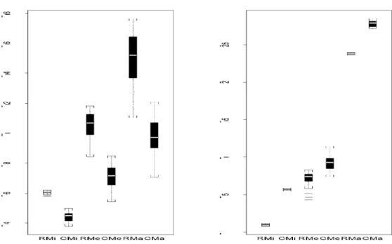
We¯ rst characterizethedistribution of theportfolios constructed at thebaseline. Figure 4 shows the distribution of the three robust and classical baseline portfolios. In this ¯ gure, the notations RMi, RMe, and RMa (CMi, CMe, CMa) stand for the robust (classical) portfolios of the three types. The plot at left shows the returns. We observe that the robust portfolios are more stable, with a distribution located at higher values and possessing smaller variability. For example, for the minimum risk portfolios, the smaller observed robust value was greater than the highest observed classical one. We also carried out a formal paired t-test to test equality of the means of the returns. For all three types of portfolios the p-value was zero against the alternative hypothesis of the robust mean return being greater than the classical one.

< < Insert Figure 4 here> >

The risks associated to the 31 portfolios are box-plotted at the right hand side of Figure 4. We also note a smaller variability of the (also smaller) robust quantities. The baseline e®ect on the portfolios may be noticed from the high variability of the returns computed for each type of portfolio. However, the robust ones showed more stability through time.

Next, we assess the distribution of the cumulative returns by examining the 100-days accumulated values associated to the 31 baseline portfolios. Table II gives summaries of the results. We observe that, for all three types, the distributions of the accumulated returns of the robust portfolios are located at the right of the classical ones. For example, the median of the central robust portfolio is 0.407, whereas the classical central portfolio distribution is located at -1.495.

< < Insert Table II here> >

(11)

were kept ¯ xed during the 100-days period. To check this assumption, we again split the data in two parts. The ¯ rst part contains 1313 observations and it is used to estimate the robust and classical MV inputs. The idea is to observe, for a given portfolio, how do the weights change as long as new data points are incorporated in the analysis. Thus, successive days were incorporated into the analyses (and the sample sizes increased to 1313 + i , i = 1; :::; 100). In this way we could assess how stable are the portfolios weights during a 100-days period. The minimum risk, the maximum return, and the \ central" portfolio are used. The compositions of the portfolios at the baseline day t = 1313 are given in Table III in the Appendix.

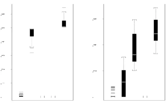
The results are that the weights are very stable for the two extreme portfolios, under both robust and classical procedures, which usually puts weight 1 to some variable. However, the weights associated with the robust and classical central portfolios are di®erent. This can be seen in Figure 5 where we boxplot the weights associated to the 5 components of the central portfolio under the robust (left) and classical (right) approaches. The robust weights presented less variability for all 5 components.

I I I

A ssessing goodness of ¯ t t hr ough simulat ions

For a ¯ xed return value the robust and the classical techniques provided di®erent risk levels. How accurate are these numbers when estimating the true standard deviation of the portfolios? This of course depends on how close to the true values are the estimated inputs used to obtain the e± cient frontier, which goes down to a realistic model and good estimators applied to the multivariate data. We now carry out two Monte Carlo experiments to investigate the accuracy of the robust and classical approaches.

(12)

To generate data which could represent some of the characteristics of ¯ nancial series we base on the real data previously used. The true model is assumed to be a multivariate normal distribution N5(µ; C) contaminated with a ¯ xed proportion

of 3% of negative and positive outliers. The outliers are obtained by adding to the randomly generated values a contaminating arbitrary value, in order to produce what is known by additive outliers (Hampel et al., 1986). For each variable these contaminating values are di®erent, and based on the atypical points observed in sample6_{. The additive outliers are a reasonable representation of the e®ect of major}

news and interventions, which do not change the data generating process, but cause large short-time e®ects. Experiment 1 puts all contamination only on the two local variables(mimicking a local turmoil); and Experiment 2 contaminatesall 5 variables, to represent periods of global crisis.

For each experiment we ran N = 500 simulations. The sample size n and C are also chosen based on the real data used in Section II: n = 1300 and C, given in (2), has the values of the estimate ^§ of the data. The true 20 parameters are thus the center µ of the multivariate distribution taken as µ = (0; 0; 0; 0; 0), and, for i ; j = 1; :::; 5, the following variances and covariances ¾i j

2 6 6 6 6 6 6 6 4

3:905 0:032 0:818 0:411 0:600 0:032 0:010 0:006 0:008 0:004 0:818 0:006 0:876 0:196 0:221 0:411 0:008 0:196 0:588 0:125 0:600 0:004 0:221 0:125 0:363

3 7 7 7 7 7 7 7 5 : (2)

(13)

I I I .a Par amet er est imat es

In the two experiments, for each simulated data set we computed the classical and the proposed robust estimates of the means and covariances. The output summa-rizing the 500 results are the mean, the standard deviation, the square root of the mean squared error (RMSE), and the median of the absolute value of errors (MAE) of the estimates of the 20 parameters.

In the ¯ rst experiment the robust procedure showed smaller bias, RMSE and MAE, in 4 out of 5 estimated means; in 3 out of the 5 estimated variances; and in 6 out 10 estimated covariances. We report in Table IV the worst cases in each class of parameters (mean, variance, and covariance), and for each estimator. The worst classical cases are in rows 1, 3, and 5. We observe the in° ated classical RMSE values implied by the large bias of the point estimates.

< < Insert Table IV here> >

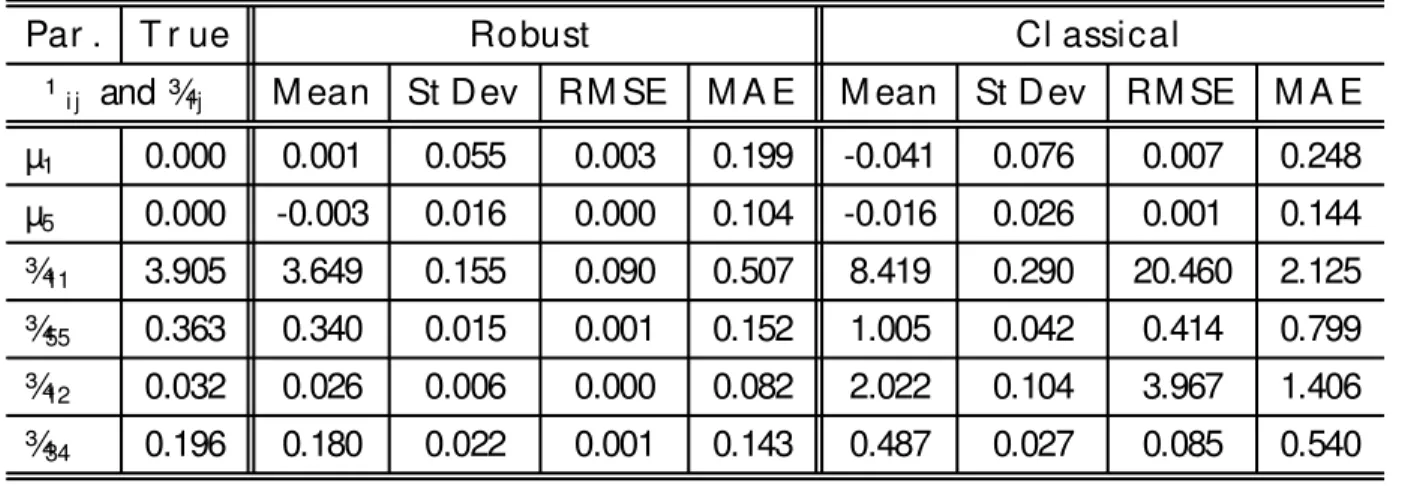
In the second experiment the robust procedure showed better RMSE and MAE performances for all 20 parameters. Some classical estimates showed very large biases, which is exactly the e®ect of the zero breakdown points. Table V shows the results for the same parameters used in previous table. For example, note the classical point estimates of ¾11, ¾55, and ¾12.

< < Insert Table V here> >

I I I .b

Est imat es of r et ur ns and r isks of por t folios

The biased estimates will also a®ect the corresponding e± cient frontiers, as the MV optimization technique is very sensitive to changes in the inputs (Michaud, 1998). We now investigate the e®ect of the robust and classical inputs on the return and risk of speci¯ c portfolios.

(14)

Their (true) compositions are given in Table VI, in the Appendix.

For each 500 simulated samplesof experiments1 and 2 of theprevioussubsection, generated according to the true model contaminated with outliers, we computed the robust and classical estimates of the covariancestructure, which are used to compute the returns and risk of the three robust portfolios and the three classical portfolios, using the true weights given in Table VI.

Table VII (Table VIII) gives the summaries of the returns (risks) of portfolios from the 500 simulations of the ¯ rst experiment. With respect to the returns, and for the minimum risk and the central portfolios, the coverage of the true values (0.0559 and 0.0774), given by the summaries in Table VII, is much better under the robust approach. For the maximum return portfolio the robust and classical summaries are very close with the median close to the true return value (0.0989). With respect to risks, the classical and the robust approaches fail to cover the true value, either under or over-estimating the risk, for all three portfolio types, except in the case of the central classical portfolio. See Table VIII in the Appendix.

< < Insert Table VII here> >

The results using data from the second experiment were very similar to those obtained using simulated data from the ¯ rst experiment. We do not present these results for the sake of brevity.

I V

Conclusions

In this paper we proposed a statistical model and estimation procedure for non normal heavy tailed multivariate data containing some proportion of atypical ob-servations. These are characteristics typically found in ¯ nancial data, in particular in emerging markets data.

(15)

that these atypical observations may tilt the orientation of the axes of the ellipsoid associated to the covariance matrix estimate.

Our robust model and estimation procedure is expected to work well when data clearly are generated from a main structure, but contain a small proportion of extreme observations, as it is usually what is observed for ¯ nancial data. In other words, the model is expected to re° ect the pattern of usual days, via the correct correlation structure, and also the e®ect of atypical days, via in° ated variances.

As any 0.5 breakdown point estimates, the procedure proposed here may give meaningless estimates if the data are in fact multivariate normal with no atypical points. For these kind of data, classical estimates based on normal model provide much more e± cient estimates. A good rule of thumb is to compare the results provided by the classical and robust techniques to better understand the data.

Several aspects of the out-of-sample performance of the robust and classical portfolios were investigated. We found that robust portfolios typically yield higher accumulated returns. Also, for any given type of portfolio (minimum risk, maximum return, central portfolio) and at any baseline time, the robust portfolios showed a more concentrated distribution with higher expected returns. We also concluded that the baseline choice has a stronger e®ect on classical portfolios. Finally, we found that the weights associated to the classical portfolios are less stable than the robust ones.

The simulations indicated that the robust approach is able to estimate the true parameters with smaller biases, and this property is re° ected on the values of the expected returns of the portfolios: More accurate ¯ gures for the portfolios in the e± cient frontier can be obtained from the robust approach.

A ppendix

1. Let x represent the n £ p data set with xi being its i -th row. Let ¹ represent its center

and § its covariance matrix. The ellipsoids are the points of constant probability density contour, or the points at the same statistical distance from the center, that is, the set f all y 2 <p_{such that (y ¡ ¹ )}0_§¡ 1_{(y ¡ ¹ ) = c}2_{g, c a real number. The choice of c}2_{= Â}2

p(®),

where Â2

p(®) is the upper (100®) quantile of a chisquare distribution with p degrees of

(16)

2. Compositions of robust and classical portfolios of Minimum risk, Maximum return, and \ central" return at the baseline t = 1313.

Table III: Portfolios' compositions at baseline t = 1313 under robust and classical esti-mation.

Return Risk IBOVESPA CDI S&P500 EAFE EMBI Minimum Risk Portfolios

Robust 0.058 0.114 0.000 0.989 0.000 0.000 0.011 Classical 0.039 0.560 0.000 0.486 0.099 0.228 0.187

Maximum Return Portfolios

Central Return Portfolio

3. Table VI gives the compositions of the portfolios in the \ true" e± cient frontier. The true inputs in the MV optimization procedure are the center (0; 0; 0; 0; 0) and the covari-ance matrix (2).

Table VI: Portfolios' compositions under the true model. True Return True Risk True Weights

Minimum Risk Portfolio

0.0559 0.0996 0.0000 0.9840 0.0001 0.0010 0.0150 Central Return Portfolio

0.0774 0.3133 0.0000 0.4926 0.0000 0.0000 0.5074 Maximum Return Portfolio

(17)

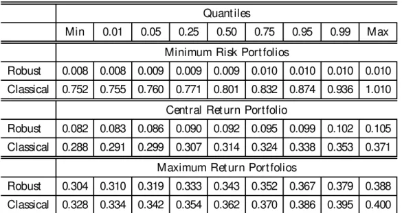
Table VIII: Distribution of risks of simulated portfolios.

Quantiles

Min 0.01 0.05 0.25 0.50 0.75 0.95 0.99 Max Minimum Risk Portfolios

Robust 0.008 0.008 0.009 0.009 0.009 0.010 0.010 0.010 0.010 Classical 0.752 0.755 0.760 0.771 0.801 0.832 0.874 0.936 1.010

Endnot es

The¯ rst author gratefully acknowledgesBrazilian ¯ nancial support from CNPq-PRONEX.

V

Refer ences

Bekaert, G., and Harvey, C. R. (1997). \ Emerging Markets Volatility" . Journal of Financial Economics.

Huber, P.J. (1981). Robust Statistics. Wiley, New York.

Johnson, R. and Wichern, D. (1990). Applied Multivariate Statistical Analysis. Prentice Hall.

Maronna, R. A. (1976). \ Robust M-estimators of Multivariate Location and Scat-ter" . The Annals of Statistics, 4, 51-56.

(18)

Michaud, R. O. (1998). E± cient Asset Management. Havard Business School Press, Boston, MA.

Reyna, F. Q., Mendes, B. V. M., (2001). \ Robust Optimal Portfolio" . Proceedings from VIII CLAPEM (Congreso Latino Americano de Probabilidad y Estad¶³stica Matem¶atica), Cuba.

Reyna, F. Q., Mendes, B. V. M., Duarte, A. M. Jr. (2000). \ Estructuracion ¶Optima de Carteras de Inversiones en el Mercado Brasile~no Usando Estimadores Robustos para la Matriz de Covarianza" . Estadistica, 51, 157, 167-186.

Rousseeuw, P.J. (1984). \ Least Median of Squares Regression" . Journal of the American Statistical Association, 79, 871-881.

Rousseeuw, P.J. (1985). \ Multivariate estimation with high breakdown point" . In

Mathematical Statistics and Applications, Vol. B, eds. W. Grossmann, G. P° ug, I. Vincze and W. Wertz. Reidel: Dordrecht, 283-297.

Rousseeuw, P.J. and Van Zomeren, B. C. (1990). \ Unmasking Multivariate Outliers and Leverage Points" . Journal of the American Statistical Association, 85, 411, 633-651.

(19)

(20)

(21)

(22)

(23)

(24)

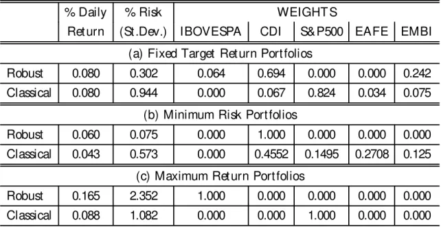
Table I:Portfolios compositions at the baseline t = 1013, based on the robust and classical inputs.

% Daily % Risk WEIGHTS

Return (St.Dev.) IBOVESPA CDI S&P500 EAFE EMBI (a) Fixed Target Return Portfolios

Robust 0.080 0.302 0.064 0.694 0.000 0.000 0.242

Classical 0.080 0.944 0.000 0.067 0.824 0.034 0.075

(b) Minimum Risk Portfolios

Robust 0.060 0.075 0.000 1.000 0.000 0.000 0.000

Classical 0.043 0.573 0.000 0.4552 0.1495 0.2708 0.125 (c) Maximum Return Portfolios

Robust 0.165 2.352 1.000 0.000 0.000 0.000 0.000

(25)

Table II: Quantiles of the distribution of the 100-days cumulative returns for the three types of portfolios.

Probabilities

0.01 0.05 0.25 0.50 0.75 0.95 0.99

Minimum Risk Portfolios (Mi)

Robust -5.8801 -3.7247 0.2054 1.4816 4.0401 10.8487 14.0901 Classical -11.4632 -8.5662 -5.7592 -1.7407 1.6105 6.9451 8.5457

Central Portfolios (Me)

Robust -11.9800 -8.7699 -3.3460 0.4071 4.3120 11.1023 17.0139 Classical -9.1792 -8.0000 -3.8494 -1.4955 2.1490 6.2649 10.6867

Maximum Return Portfolios (Ma)

(26)

Table IV: Results for 6 parameters (out of 20) from Experiment 1. Contamination pro-portion is 3% on \ local" variables.

Par . T r ue Robust Cl assical

µi and ¾i j M ean St Dev RM SE M A E M ean St D ev RM SE M A E

µ1 0.000 -0.003 0.056 0.003 0.198 -0.001 0.080 0.006 0.228

µ5 0.000 0.000 0.017 0.000 0.107 0.000 0.016 0.000 0.103

¾11 3.905 3.690 0.162 0.073 0.468 8.135 0.250 17.954 2.058

¾55 0.363 0.343 0.015 0.001 0.143 0.363 0.013 0.000 0.092

¾12 0.032 0.027 0.006 0.000 0.078 1.915 0.081 3.550 1.369

(27)

Table V: Results for 6 parameters (out of 20) from Experiment 2. Contamination pro-portion is 3% on all 5 variables.

Par . T r ue Robust Cl assical

¹i j and ¾i j M ean St Dev RM SE M A E M ean St D ev RM SE M A E

µ1 0.000 0.001 0.055 0.003 0.199 -0.041 0.076 0.007 0.248

µ5 0.000 -0.003 0.016 0.000 0.104 -0.016 0.026 0.001 0.144

¾11 3.905 3.649 0.155 0.090 0.507 8.419 0.290 20.460 2.125

¾55 0.363 0.340 0.015 0.001 0.152 1.005 0.042 0.414 0.799

¾12 0.032 0.026 0.006 0.000 0.082 2.022 0.104 3.967 1.406

(28)

Table VII: Distribution of returns of simulated portfolios.

Quantiles

Min 0.01 0.05 0.25 0.50 0.75 0.95 0.99 Max Minimum Risk Portfolios