António Afonso, Jorge Silva
Effects of euro area monetary policy on
institutional sectors: the case of Portugal
WP15/2017/DE/UECE
_________________________________________________________
Department of Economics
W
ORKINGP
APERS1
Effects of euro area monetary policy on institutional sectors: the
case of Portugal
*António Afonso,
$Jorge Silva
+ #July 2017
Abstract
We study the effects of the euro area monetary policy on the institutional sectors in Portugal during the period 2000:4-2015:4. Our results show that the single monetary policy affected some variables that are proxies for the funding of each institutional sector of the economy: general government, other monetary financial institutions, non-financial corporations, households and the external sector. The period of the economic and financial adjustment programme influenced all institutional sectors, and financial integration in the euro area had an effect on the funding for the economy: there was a reduction of long term-to-GDP ratio, external funding to the Portuguese other MFIs, and new loans to households
Keywords: monetary policy, euro area, Portugal, non-conventional instruments, institutional sectors, financial integration
JEL:C20, E44, E52, E62, G01
* We thank useful comments from Goran Vukšić and from participants at the 6th UECE Conference on Economic
and Financial Adjustments, 2017. The opinions expressed are those of the authors and are not necessarily those of the respective employers.
$ ISEG – School of Economics and Management, Universidade de Lisboa; REM – Research in Economics and
Mathematics, UECE. UECE – Research Unit on Complexity and Economics is supported by Fundação para a Ciência e a Tecnologia. email: aafonso@iseg.utl.pt.
+ ISEG – School of Economics and Management, Universidade de Lisboa, email:jorgefariasilva@gmail.com. # Portuguese Parliament, Parliamentary Technical Budget Support Unit, Lisbon.
2
1. Introduction
The debate about the advantages and disadvantages of a single monetary policy in the euro area has been an important theme of political and academic discussion during the last decades.
The single monetary policy of the European Central Bank (ECB) may not fit all countries equally, so it is necessary to analyse its effects on specific countries separately. In this paper, we focus on Portugal, a small open economy, which is an interesting case study since it faced in the beginning of the 2010s high external imbalances, high public debt, low economic growth and an economic and financial adjustment programme. Therefore, we assess the impact of a tightening or accommodative monetary policy on Portugal, during the period 2000:4-2015:4. We take into account the euro area monetary variables, the unconventional monetary policy instruments and changes in the transmission mechanism.
In addition, monetary policy developments may trickle down differently across institutional sectors. Hence, we also study the impact of monetary policy on the relation between financial accounts of the institutional sectors. We consider the flows related to financial accounts for each of the five institutional sectors: general government, other monetary financial institutions (MFIs), households, non-financial corporations (NFCs) and the external sector. Consequently, we assess the impact of the monetary policy variables on these flows. In this way, a modified Taylor rule would not be appropriate to assess the impact of monetary policy due its sector encompassing approach.
Our main results are as follows: i) monetary policy influenced all institutional sectors; ii) financial integration in the euro area had an effect on the funding for the Portuguese economy: long term public debt ratio, funding from the Portuguese central bank to the other MFIs, external funding, and new loans to households and NFCs; and iii) the period of the economic and financial adjustment programme (EFAP) impacted all institutional sectors: there was a reduction of long term-to-GDP ratio, external funding to the Portuguese other MFIs, and new loans to households.
The paper is organised as follows. Section two presents a literature review. Section three addresses the methodological framework. Section four presents and discusses the results. Section five is the conclusion.
2. Literature Review
In order to place our paper in the literature, there are some studies about monetary policy focussing on several different issues. For instance, notably the Taylor rule as a benchmark to
3
assess the decisions of the central banks and the features of the European Monetary Union (EMU); the recent literature on the relationship between the financial crisis and the European sovereign debt crisis; the impact of non-conventional instruments of monetary policy on the economy; and financial markets and government bond yields.
2.1. Period before the financial crisis
Taylor (1993) explained the difference between discretion and policy rules in monetary policy. Under discretion, the setting of instruments is determined from scratch each period and without a contingency plan for the future. On the other hand, under a policy rule, there are feedback rules that respond to changes in unemployment and inflation. The policy rule does not have to be a mechanical formula. The Taylor rule presented in (1), over the period 1987-1992, defined that changes in the federal funds rate were determined by the evolution of the output gap and the deviation of inflation from the target:
= + 0.5 + 0.5 − 2 + 2 (1)
where is the federal funds rate, is the deviation of real GDP from a target, is the rate of inflation and 2 is a parameter close to the assumption of steady state growth for the US economy. Furthermore, the author took into account the transition from one policy rule to a new policy rule, such as a disinflation process and changing the inflation target rate from 5% to 2%. The author presented two case studies – German unification and the 1990 oil price shock – which illustrate how a policy rule cannot be applied mechanically. For example, the temporary increase of the deflator in 1990 during some months of the Iraqi war was higher than the fall of the real output, suggesting a misleading increase of the federal funds rates.
Puri et al. (2011) studied the retail bank lending in Germany during the period 2006-2008 based on loans applications and loans granted.1 The aim of the study was to assess the impact of the US financial crisis on the German retail bank lending. It is important to stress that some German banks invested substantially in the USA and consequently were affected by the US financial crisis. The authors also made a split between supply and demand side effects. There was an overall decrease in demand, which includes borrowers of affected and non-affected banks. Regarding the supply side, the results showed the US financial crisis contracted the supply of retail lending in Germany. In addition, the affected banks by the financial crisis rejected significantly more loans applications than non-affected banks, in particular small and liquidity constrained banks.
4
2.2. Period during and after the financial crisis
Gaspar and Issing (2011) presented the role of the ECB for monetary policy in the euro area as well as its responsibilities defined by the Treaty on the Functioning of the European Union (TFEU). Price stability over the medium term is the sole responsibility for the ECB’s monetary policy. However, the aim of price stability highlighted some tension between single monetary policy and national economic policies and financial stability, which were known during the financial and economic crisis 2007-2011.
Nechio (2011) applied a version of the Taylor rule not only to the euro area as a whole, but also to each country. The target rate of the ECB seemed to be in line with the Taylor rule recommendation over the period 2001-2011. However, this rule recommended negative nominal interest rates in the case of the peripheral countries since the financial crisis. Nechio (2011) concluded that a single policy rate did not fit all member states because the core countries were recovering, while peripheral countries had large unemployment gaps.
Lane (2012) assessed the European sovereign crisis and the impact of negative macroeconomic shocks. When the crisis occurred, the euro area presented a low degree of fiscal and banking union. The author identified risks of multiple equilibria when sovereign debt is high. The “bad equilibrium” leads to the risk of self-fulfilling speculative attacks, that is, an increase in perceptions of default risk induces investors to demand higher yields. Therefore, the rollover of public debt is more difficult and makes default more likely. On the other hand, the “good equilibrium” allows that the investors do not need to fear that a country is pushed into an involuntary default by inability to rollover public debt. Consequently, it was required policies to encourage the “good equilibrium”. A larger fund of the European Stability Mechanism as well as the ECB’s program to purchase sovereign bonds could attenuate such dire market conditions.2
Schabert (2014) assessed how optimal monetary policy is constrained by credit market frictions and what is the role for central bank asset purchases. The author used a sticky price model where credit market is distorted when borrowing between private agents is constrained by available collateral. In this situation, optimal monetary policy ignores credit frictions when is conducted in a conventional way with only one instrument (i.e. short-term nominal interest rate). However, the central bank can control both the price and the amount of money when collateral is a bounded set of eligible assets. In this circumstance, the central bank can
5
purchase secured loans at a more favourable price (higher than market price) in order to alleviate the severity of borrowing constraints, reduce the lending rate and stimulate the credit market.
Altavilla et al. (2014) studied the macroeconomic effects of the Outright Monetary Transaction (OMT) programme announced during the period July-September 2012. The authors used high-frequency data, a multi-country model describing the macro financial linkages and focused on four countries: France, Germany, Italy and Spain. Regarding the 2-year government bond yields, the OMT announcements decreased the Italian and Spanish yields by about 200 basis points, and left unchanged the bond yields of the same maturity in Germany and France. The reduction of the 10-year government bond yields in Italy and Spain (about 100 basis points) were smaller than the decrease in 2-year bond yields, which is consistent with the target of this monetary policy measure, i.e. explicit focus on bonds with remaining maturities of up to 3 years. Regarding the macroeconomic effects, the decrease in bond yields due to the OMT announcements was associated with a substantial effect on credit, economic growth and prices in Italy and Spain, but relatively limited spillovers in France and Germany.
Ferrando et al. (2015) studied the effects on the small firms’ financing of sovereign stress and of the unconventional euro area monetary policy during the period of the debt crisis (2009Q1-2014Q1). It is import to stress that small firms are more likely to be credit constrained when banks adjust portfolios due to negative shocks on balance sheets. The authors concluded that small firms in the stressed countries were more likely credit rationed through both the price and quantity, as well as increased debt securities.3 However, there was evidence that the OMT decreased the share of credit-rationed firms.4 Therefore, firms with improved outlook were more likely to benefit from easier credit conditions. Even in the stressed countries, the first semester after the announcement of the OMT programme had a positive impact credit access. In addition, firms were more likely to reduce government‑subsidized loans.
Garcia-de-Andoain et al. (2016) studied the effect of the liquidity provision by the ECB on the overnight unsecured interbank markets. The authors used data from the payment system TARGET2 for the period 2008-2014 and a structural vector auto-regression. They report evidence that the ECB had acted as lender-of-last-resort for the banking system, in
3 This study considered as “stressed countries” Greece, Ireland, Italy Portugal and Spain.
4 The OMT Program was announced on 2nd August 2012 and technical framework on 6th September 2012. For
6
spite of no explicit reference to this function on the ECB’s mandate. In addition, there were two effects of central bank liquidity: the replacement of the demand for liquidity in the interbank market (financial crisis 2008-2010), and an increase in the supply of liquidity in the interbank market in Greece, Italy and Spain (the debt crisis 2011-2013).
Andrade et al. (2016) analysed the effects of the expanded asset purchase programme (APP) on the macro economy, sovereign yields and transmission channels. The APP was announced in January 2015 and it decreased sovereign yields on long-term bonds, as well as increased the share prices of banks, in particular banks with higher weight of sovereign bonds in portfolios. The results are consistent with the portfolio rebalancing channel due to the removal of duration risk as well as the relaxation of leverage constraints for financial intermediaries. The macroeconomic impact of the APP may be sizable due to ease credit conditions and reanchoring inflation expectations towards its medium-term inflation objective.
Additionally, Afonso and Jalles (2017) report that in the aftermath of the 2008-2009 economic and financial crisis the quantitative easing measures implemented by the ECB became relevant determinants of the yield spreads. In fact, using a time-varying analysis, the Covered Bond Purchase Programme contributed to reduce yield spreads in all euro area countries, particularly in the crisis period, 2011-2013, while longer-term refinancing operations contributed to reduce yield spreads in most countries.
3. Methodological framework
According to the TFUE, the sole responsibility for the ECB is the price stability over the medium term. However, the most appropriate monetary policy for the euro area as a whole may not be the most appropriate for each country. Price stability is defined as inflation rates below, but close to, 2% over the medium term. Figure 1 compares the inflation rate in the euro area and Portugal. The average inflation in Portugal (2.09%) was higher than in the euro area (1.70%) in the period 1997-2016.
[Figure 1]
Some previous literature assessed monetary policy through the simple Taylor rule. However, the period 1999-2016 includes both normal times and the zero lower bound. Consequently, some papers used modified Taylor rules (e.g. non-linear Taylor rule) in order to assess monetary policy in a context of the zero lower bound. Nevertheless,
7
Bernanke(2015) warned about the complexity of the underlying judgements to make decisions and that such simple rule does not provide guidance when the predicted rate is negative. In this way, monetary policy decisions are more complex than a simple Taylor rule and monetary policy should be systematic.
3.1 Non-conventional instruments of monetary policy
We can split the ECB’s monetary policy into two periods, where the introduction of non-conventional instruments in July 2009 was the determinant factor. It is important to stress the difference between the periods before and after the economic and financial crisis in 2007-2009.
The period between the introduction of the euro and the financial crisis was characterized by a reduction of government bond yields in euro area countries as well as narrower yield spreads among countries, higher economic growth, easier external financing and increasing external imbalances. There were only conventional instruments of monetary policy.
Afterwards, the economic and financial crisis influenced the core countries of the euro area, in particular via a direct impact on bank balance sheets. In the aftermath of the crisis, there was evidence of fragmentation (i.e. decrease of financial integration) on the European financial markets, which generated the sudden stop in the capital inflows to the European external deficit countries.
The financial crisis was the main factor for the introduction of non-conventional instruments by the ECB, and each of the instruments had a specific aim. Table 1 presents the non-conventional instruments, the announcement date and the period of implementation and their main features. The non-conventional instruments included the following programmes instruments for the period 2009-2016 (Table 1 and Figure 2).
Covered bond purchase programme (CBPP1) - the aim of supporting a specific financial market segment that was important for the funding of banks and that was particularly affected by the financial crisis. The nominal amount (EUR 60 billion) has been purchased on the primary and secondary markets. The Eurosystem intends to keep the purchased covered bonds until maturity.
[Table 1] [Figure 2]
The Securities Markets Programme (SMP) aimed at ensuring liquidity and depth in malfunctioning segments of the debt securities markets as well as restoring an appropriate transmission mechanism of monetary policy. In the beginning, there was no central bank liquidity change because the purchases of debt securities were sterilised. In addition, the SMP
8
did not alter the stance of monetary policy. This programme purchased sovereign debt on the secondary market (of Ireland, Greece, Spain, Italy and Portugal), with the ECB holding sovereign debt to maturity and suspending sterilisation in June 2014.
The Covered bond purchase programme 2 (CBPP2) aimed to ease funding conditions for credit institutions and enterprises as well as to encourage credit institutions to maintain and expand lending. This programme included purchases on the primary and secondary markets. The Eurosystem intends to keep these bonds until maturity.
The OMT aimed at safeguarding an appropriate monetary policy transmission and the singleness of the monetary policy as well as replacing the SMP. It will be considered for countries with macroeconomic adjustment programmes or precautionary programmes. There is a strict conditionality attached to a European Financial Stability Facility/European Stability Mechanism (EFSF/ESM) programme. The focus is on the sovereign bonds with a maturity of between one and three years and the transactions are fully sterilized.
The targeted longer-term refinancing operations (TLTROs) operations aimed at providing financing to credit institutions for periods of up to four years. Therefore, they allow offering long-term funding at attractive conditions to banks in order to ease private sector credit conditions and stimulate bank lending to the real economy. In this way, the TLTROs reinforce the transmission of monetary policy. There were two series of TLTROs: a first series announced on 5 June 2014 (TLTRO I) and a second series on 10 March 2016 (TLTRO II). The amount that banks can borrow is linked to their loans to households (excluding loans to households for house purchase) and NFCs.
In addition, the expanded APP was decided on 22 January 2015 and aimed at sustaining the adjustment of inflation path. It included the current programmes at that date and added another programme in March 2016.
The third Covered Bond Purchase Programme (CBPP3) had the aim of enhancing the transmission of monetary policy, facilitating credit provision to the euro area economy, generating positive spillovers to other markets and contributing to a return of inflation rates to the medium term target. The Eurosystem central banks purchase eligible bonds in the primary and secondary markets.
The Asset-backed securities purchase programme (ABSPP)’s purpose was enhancing the transmission of monetary policy, facilitating credit provision to the euro area economy and generating positive spillovers to other markets. The ABSPP also helped banks to diversify funding sources and stimulated the issuance of new securities, by purchasing in both the primary and secondary ABS markets.
9
The Public sector purchase programme (PSPP) aims at fulfilling the price stability mandate and provide monetary stimulus in a context of the zero lower bound. The PSPP makes access to finance cheaper for households and firms in order to support consumption and investment. Therefore, the improvement of economic activity contributes to a return of inflation rates towards the medium term target. There are only secondary market purchases.
The Corporate sector purchase programme (CSPP) aims to further strengthen the pass-through of the Eurosystem’s asset purchases to the financing conditions of the real economy. In addition, the CSPP provides further monetary policy accommodation and helps inflation rates return to the medium term target. The purchases will be conducted in the primary and secondary markets and non-bank corporations established in the euro area issue the euro-denominated bonds.
Figure 3 presents the total outstanding of the ECB’s purchases. The PSPP presents the largest outstanding and it has been increasing since the introduction in March 2015. The SMP presents the second largest outstanding, but it has been decreasing since the end of this programme in the summer 2012 due to the maturity of some government bonds (Figure 3 and Figure 4).
[Figure 3] [Figure 4]
Furthermore, when a solvent financial institution faces temporary liquidity problems, it is possible to obtain a provision of credit by the Eurosystem national central bank: the Emergency Liquidity Assistance (ELA). This instrument is not a monetary policy instrument, but it increases the central bank money. Therefore, any costs arising from the provision of the ELA will be incurred by the national central bank.
Sterilisation
During the implementation of non-conventional instruments of monetary policy, it is important to identify two periods: full sterilization and non-sterilization. In the case of full sterilization, the ECB conducted specific operations with the aim of re-absorbing the liquidity injected through the purchases underlying non-standard instruments of monetary policy, avoiding the variation of the money supply.
Table 2 presents the date of 5 June 2014 when the ECB suspended sterilisation of non-conventional instruments. This date is known as the beginning of the quantitative easing.
10
Hence, the Taylor rule approach may not be useful to assess the impact of monetary policy on the Portuguese economy due to a large range of non-conventional instruments and zero lower bound.
Finally, we can observe that the disaggregation of the ECB’s balance sheet changed during the period 1999-2015. Figure 5 includes the non-conventional instruments on the balance sheet: lending to euro area credit institutions related to monetary policy operations denominated in euro and securities of euro area residents denominated in euro. The increase of these assets was offset by an increase of the banknotes in circulation and liabilities to euro area credit institutions related to monetary policy operations denominated in euro.
[Figure 5]
3.2 Disaggregation by institutional sector Zero lower bound
Gaspar (2016) presented the role of monetary policy in two different contexts: in normal times, monetary policy is a shock absorber while in the zero lower bound monetary policy is a shock amplifier. In normal times, a negative demand shock pressures inflation downward and monetary policy cuts nominal interest rates with the aim of decreasing real interest rates and depreciating exchange rate. Therefore, it is expected that higher nominal GDP and monetary policy is a shock absorber.
However, in the case of the zero lower bound, a negative demand shock pressures inflation downward, but the central bank cannot decrease nominal interest rates because monetary policy is at the effective lower bound (i.e. nominal interest rates close to zero). Consequently, there are higher real interest rates and exchange rate appreciation, which impact negatively on nominal GDP and public and private debt ratios. In fact, there is a vicious cycle with stronger negative demand shock and decrease of inflation and nominal GDP. For that reason, monetary policy is a shock amplifier. Therefore, a coordinated policy, including monetary policy non-conventional instruments, fiscal policy (e.g. infrastructure investment) and structural reforms (labour and product market and tax system) is paramount.
Demand, supply and monetary policy
There is consensus that monetary policy has real effects on the economy at least in the short run. The transmission channels of monetary policy can influence aggregate demand. In addition, a prolonged and deep recession as well as a depressed demand has a negative impact on the trajectory of potential output. Delong and Summers (2012) studied the role of fiscal
11
policy in a depressed economy (the United States). In the case of short-term nominal interest rates at the zero lower bound, with high cyclical unemployment, large output gap and excess capacity, an increase in government expenditure would not be either offset by monetary policy or neutralized by supply-side bottlenecks.
Therefore, it is important to stress the negative effect of depressed aggregate demand on the aggregate supply and potential output. In fact, even with a small amount of hysteresis, an expansionary fiscal policy may be self-financing. If it is not, expansionary fiscal policy may raise the present value of future potential output. In this way, the zero lower bound requires coordination between monetary and fiscal policy.
The ECB monetary policy decisions can affect the economy through several channels: the interest rate, the bank lending and the balance sheet, the exchange rate, the asset prices, the wealth effect, as well as the Tobin’s ratio between thephysical asset's market value and the replacement cost of capital. In addition, we can connect channels and institutional sectors: e.g. bank equity prices, portfolios flows, exchange rate, sovereign yield, wages and available income. According to economic theory, we elaborate on how monetary policy can impact on each institutional sector.
General government
The ECB monetary policy has the sole responsibility of price stability, but some monetary policy decisions impact on sovereign yields. There have been non-conventional instruments that eased the pass through of monetary policy and reduced government bond yields (e.g. the SMP and OMT announcement). In fact, the ECB holds public debt under non-conventional measures. Therefore, monetary policy decisions can impact on the yield curve and the rollover of public debt and the funding of the budget deficit may be affected.
Other monetary financial institutions
The monetary policy decisions can impact on the structure of banks’ balance sheets. For that reason, tighter (or easier) monetary policy can increase (decrease) interest rates along the yield curve and decrease (increase) the price of financial assets.
On the assets side, it is important to decompose the amount of credit allocated to the mortgage credit, which is more related to non-transactional goods and services, and the amount allocated to the NFCs. Furthermore, the stock related to the non-performing loans (NPLs) can impact on decisions’ banks to accept new loans. Additionally, monetary policy can impact on the amount of public debt on the balance sheets of the other MFIs.
On the liabilities side, monetary policy can change the yield curve, which may be important for the evolution in the composition between deposits, wholesale funding, equity
12
and bonds. In addition, loans to NFCs and households may be essential for investment (supply side) and private consumption, respectively. Furthermore, the criteria for eligible assets for monetary policy operations is defined by the ECB and impacts on the other MFIs’ decisions. Holdings of assets included in the set of eligible assets may be used as collateral for monetary policy operations.
Households
Monetary policy can impact on interest earnings and payments. The difference between earnings and payments depends on the stock of financial assets (deposits and bonds) and liabilities (loans), as well as the interest rate level. In addition, monetary policy can impact on the yield curve slope, new loans, NPLs and the amount of saving. The money market interest rates can impact on portfolio savings (e.g. deposits, bonds, bills, shares, public debt certificates). Therefore, it is interesting to assess how much monetary policy impacts on deposits (asset), loans (liability) and available income.
Non-financial corporations
Monetary policy impacts on the balance structure through the interest rate and price effects. The ratio between loans and equity is an indicator about the main source of funding. Additionally, economic growth and monetary policy stance may impact on NPLs. Investment is a key determinant for the stock of capital, which is an input to the production function (aggregate supply). Therefore, monetary policy can affect potential output through real investment.
External balance
A tighter (or easier) monetary policy can appreciate (or depreciate) both the nominal and real exchange rate in the short term.5 However, according to the interest rate parity a positive (negative) difference between nominal interest rates of two countries with different currencies is the result of depreciation (appreciation) of the nominal exchange rate in the country with higher (lower) nominal interest rates and higher (lower) inflation rate over the long term. Therefore, the euro area monetary policy can impact on exchange rate in the short and long term with the trading partners located outside the EMU.
International investment position
In addition, monetary policy can impact on the composition of the external balance, balance of payments, financial accounts and international investment position (IIP). A tighter (easier) monetary policy can impact on interest rates in monetary and financial markets. In
13
this way, the wealth effect defines that higher (lower) interest rates along the yield curve mean lower (higher) asset prices, i.e. prices of bonds and shares. In addition, the IIP is presented on market value. The price effect may vary along time, which includes assets held by residents and liabilities held by non-residents. Additionally, the IIP is affected by the exchange rate.
4. Empirical analysis
Concerning the Portuguese economy, we have as sources the quarterly national accounts from Statistics Portugal (INE) as well as the financial accounts from the Portuguese central bank (Banco de Portugal). In addition, we collected a database for the total outstanding of conventional and non-conventional instruments of the ECB’s monetary policy.
Our set of independent variables includes control variables as well as variables related to monetary policy: 3-month Euribor rate, slope of the yield curve (difference between 12-month Euribor and 3-month Euribor rate), the interest rate on the main refinancing operations, the corridor between deposit and lending facilities interest rates, the amount of non-conventional instruments, monetary aggregates, exchange rate and the SMP period.
The Portuguese economy has presented a deterioration in terms of the ratio between financial assets and financial liabilities. Specifically, households reported the strongest deterioration due to the decrease of the deposits-to-loans ratio. The change in the structure of stocks of financial accounts (i.e. liabilities and assets) of the institutional sectors is achieved through financial flows.
4.1. Impact of the euro area monetary policy, by institutional sectors
In this subsection we assess if monetary policy variables have an impact on the relevant variables of each institutional sector. We consider a large range of monetary variables: the key ECB interest rates, monetary market interest rates and the non-standard instruments. Consequently, the set of independent variables includes both monetary and non-monetary variables, as well as external and domestic variables. We use the variables in differences in order to avoid non-stationary.
4.1.1. General government
Equation (2) decomposes the yield spread ( ) between the Portuguese and the German 10-year sovereign yield. It takes into account the decomposition of the spread ( ) between the Portuguese 10-year government yield and the average
14
10-year sovereign yield on a set of the peripheral countries (Italy/Ireland/Spain), as well as the spread ( ) of this average vis-à-vis the 10-year Bund yield:
= + . (2)
It is important to stress that during the period 1996Q1-2009Q4 the yield spread between the Portuguese sovereign yield and the average of the other peripheral countries was around zero (average = 0 basis points, see Figure 6). Interestingly, Coronero (2016) presented a decomposition of the yield spread, identifying the shadow spread. In the context of a lower zero bound the German 10-year sovereign yield is constrained and the yield spread is compressed. However, different economic fundamentals (sovereign risk) between countries remain in spite of the lower zero bound. In this way, the shadow spread is the sovereign spread that would be observed in the absence of the lower bound.
[Figure 6]
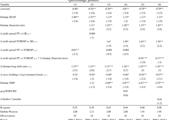
Additionally, we estimate the determinants of the share of long-term public debt-to-total public debt in the Portuguese case. Equation (3) presents the q-o-q variation of the share of long term public debt:
!"#$% !!#!&"− !'("#$% !'(!#!&") ∗ 100 = ,-+ ,. /0 1+ , 23 0 _/0 1+ 5 . (3)
The Portuguese long term debt-to-total public debt ratio increased during the period after the financial crisis. In addition, the dependent variable decreased due to the German ratio of long term securities-to-total public debt, which may be a benchmark for the euro area, and the sovereign yield spread between the peripheral countries (Italy/Ireland/Spain) and Germany. When this spread was lower it was easier to roll over public debt, which decreased the weight of long term debt securities.
[Table 3]
On the other hand, financial integration in the euro area government bond had a negative impact on the dependent variable, which means that it was easier to roll over public debt during periods of increasing financial integration. During the SMP period, there was a reduction of the weight of long-term bonds due to increasing long-term sovereign yields. The sovereign yield spread between Portugal and Italy/Ireland/Spain had a negative statistically significant effect before the financial crisis, which may have been associated with country specific difficulties to issue long term sovereign bonds. During the EFAP, there was a reduction of long term debt due to funding from the EU/IMF loans. In addition, the exchange rate, and the Euribor rate were not statistically significant.
15
4.1.2. Other monetary and financial institutions
In this institutional sector, liabilities and assets had a different composition throughout the period of analysis (Figure 7). Funding from the non-resident financial institutions decreased after the financial crisis, but deposits and funding from the Portuguese central bank offset that difference.
Concerning lending margins, loans to NFCs had higher profitability than loans for housing purposes. However, there was a strong increase of NPLs in particular related to NFCs (Figure 8).
[Figure 7] [Figure 8]
Demertzis and Wolff (2016) discussed the impact of the ECB’s quantitative easing on bank profitability. They mentioned three channels: weakening the exchange rate (exchange rate channel), decreasing the long-term interest rates, improving investment conditions and disincentivising savings (interest rate channel), and driving investors into riskier investments while the ECB purchases safe long-term assets (portfolio rebalancing channel). However, the authors stressed the effects of the two main channels: weaker exchange rate as well as lower sovereign bond yields. In fact, banks did not shed sovereign debt at a significant scale and bank profitability was squeezed by quantitative easing, while additional purchases of corporate bonds can reduce financial margins.
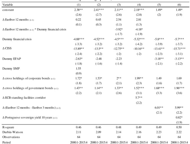
Regarding the other MFIs, we estimate two important components from the liability side: liabilities vis-à-vis the Portuguese central bank and non-resident institutions. In equation (4) 67 876797 : 0 _ ;<= ; is the q-o-q variation of the liabilities of the Portuguese other MFIs vis-à-vis residents. In this variable residents include other MFIs and non-monetary financial institutions. The set of independent variables include both non-monetary and non-monetary variables:
67 876797 : 0 _ ;<= ; = μ-+ μ.@/0 1+ μ2A 0 _/0 1+ B . (4)
Table 4 presents the results for the determinants of external funding, i.e. liabilities of the resident other MFIs vis-à-vis non-residents. Regression 6 in Table 4 shows there was a reduction of external funding due to financial systemic stress in Europe.6 During the period
after the financial crisis the dependent variable decreased, in particular a deeper reduction took place during the EFAP. However, external funding increased due to financial integration
16
on government debt in the euro area, the slope of yield curve on the monetary market and the 10-year government yield. In addition, there was statistical significance of the standing facilities corridor, 12- month Euribor rate after the financial crisis and financial integration of corporate bonds (regression 4).
[Table 4]
In equation (5) 67 876797 :C0 D ; E F is the y-o-y variation of the assets of
Banco de Portugal à-vis resident other MFIs (i.e. liabilities of the resident other MFIs
vis-à-vis the Portuguese central bank):
67 876797 :C0 D ; E F G- G.@
/0 1
G2A
0 _/0 1
B . (5) Funding from the Portuguese central bank includes the main refinancing operations and longer term refinancing operations. The dependent variable was positively explained by the systemic stress in Europe (Table 5). However, central bank funding was negatively explained by the current account variation, financial integration in the euro area sovereign bonds, 3-month Euribor rate and new deposits from households. These results are according to economic theory, i.e. when external funding was expensive or unavailable, the central bank offset funding to the Portuguese other MFIs. In addition, higher new deposits from households and higher current account balances reduced funding requirements for the Portuguese other MFIs.
[Table 5]
4.1.3. Households
The loans-to-deposits ratio is essential to assess the households’ financial accounts. Regarding interests, earnings had been higher than payments, but in some periods that was only a small difference. Concerning liabilities, housing loans are the main component (Figure 9), but there was a decrease in this item after the beginning of the EFAP.
[Figure 9]
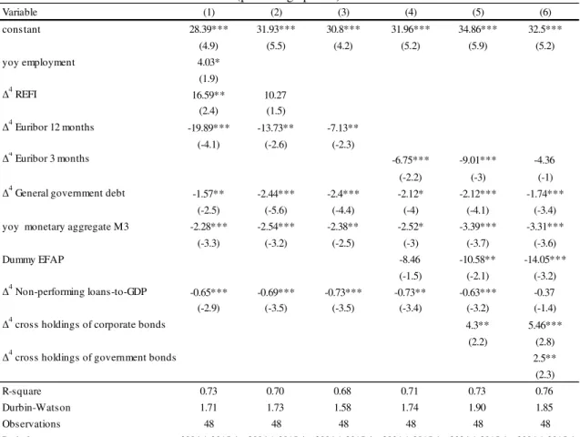
Equation (6) specifies the estimation for the y-o-y variation of new loans to households:
H I_6J H:K0 ; K0 =; L- L.M/0 1 L2N 0 _/0 1 O . (6) Regarding new loans to households (Table 6), there was a positive impact from financial integration in the euro area measured by either cross holdings of corporate bonds or cross holdings of government bonds (regression 6). In addition, there was a negative effect of the monetary aggregate M3 growth and during the EFAP period. In addition, the public debt-to-GDP ratio variation presented evidence of a crowding out effect of household’s new loans.
17
[Table 6]
4.1.4. Non-financial corporations
In this institutional sector, we assess the decomposition of assets and liabilities. Concerning liabilities, the share of loans declined after 2008 (Figure 10).
[Figure 10]
In equation (7), H I_6J H:< < < < ; is the y-o-y growth of new loans to NFCs. H I_6J H:< < < < ;= P-+ P.Q/0 1+ P
2 0 _/0 1+ R . (7)
The estimation results show that new loans to NFCs were positively affected by the period of the EFAP, Portuguese 10-year sovereign yield, PSI-20 index and financial integration in the euro area corporate bonds (Table 7). During the EFAP, there was the EU/IMF funding to the general government, which may have meant absence of crowding out effects on new loans to NFCs. On the other hand, in periods of financial stress in Europe, public debt was the safe haven and consequently there were reductions in sovereign yield and new loans to NFCs. An increase in the PSI-20 led to a rise of the market value on equity, i.e. it suggested easier access to new loans and higher expected future profits. Increases of NPLs during the previous quarter had a positive impact on the new loans, which may have been a signal of recovery in the credit market for the following periods. Financial integration measured by cross holdings of corporate bonds increased the dependent variable, which was a proxy of financial integration for the private sector. The increase of total NPLs in the previous quarter suggested a rise in the new loans to NFCs, which may be explained by the fact that loans to this institutional sector were more profitable than loans to households.
[Table 7]
However, there was a decrease of the dependent variable due to the Euribor, which was a basis for interest rates on new loans. Furthermore, higher systemic stress in Europe was a proxy for the constraints on the Portuguese other MFIs to borrow external funding and consequently providing fewer new loans to NFCs.
4.2. Impact of the euro area monetary policy on external accounts 4.2.1. External balance and terms of trade
The terms of trade compare the path between export prices and import prices. The increase of the money supply in the euro area impacts the nominal and real exchange rate in the short term. However, the depreciation of exchange rate leads to higher prices of imports
18
and lower prices of exports. There is an effect on the trade balance through two opposite effects: the increase of real exports and decrease of real imports, as well as the deterioration in the terms of trade with a negative impact on the trade balance. Figure 11 shows the difference between the trade balance (which is a nominal variable) and “trade balance” with exports and imports in volume.7 There was a rebalancing during the EFAP and a positive effect of the terms of trade.
[Figure 11]
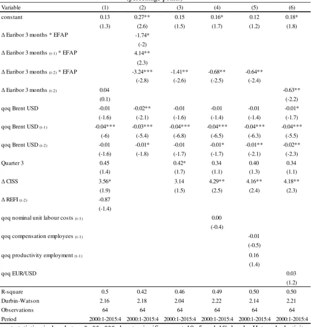
In equation (8), the dependent variable is the q-o-q variation of the terms of trade. 9 _9 S: 0 D = T-+ T. /0 1+ T2U 0 _/0 1+ R. (8)
Our results (regression 6) show the negative effect of the lagged 3-month Euribor rate and oil prices (Table 8). Therefore, an increase of commodities may have been an upward pressure on inflation and the ECB increased the interest rates in order to subdue inflation. Consequently, there was an increase of the 3-month Euribor rate, as well as a negative impact on the terms of trade. In addition, the coefficients of Brent prices were negative, which mean that there was not a complete pass through from the oil prices spike to the exports deflator. Therefore, an increase in the oil prices had a stronger impact on the imports deflator than on the exports deflator. The impact of the oil prices in the previous quarter was stronger than the current quarter. The systemic stress in Europe had a positive effect in the terms of trade. In fact, there was a negative correlation between the q-o-q change in the oil prices and the q-o-q change of the CISS. In addition, the pass through from imports deflator to the exports deflator was not complete. In this way, higher CISS was correlated to lower imports deflator, which was beneficial to the trade of terms. Finally, the exchange rate, unit labour costs, compensation of employees and labour productivity had no statistical significance. In this way, the terms of trade were mostly determined by oil prices recorded in the previous quarter.
[Table 8]
4.2.2. International investment position: price variation
The IIP variation is decomposed into flows, exchange rate effect, price effect and other adjustments. We focus on the price effect, which may be impacted by the ECB monetary policy stance. The price effect is determined by changes in the market value on assets and liabilities. In this way, monetary policy can impact on securities prices and consequently on the IIP. There was a sizeable price effect in some quarters (Figure 12).
7 The trade balance is a nominal indicator (nominal exports – nominal imports). However, we present the balance
19
[Figure 12]
In equation (9) the dependent variable is the price effect of the IIP variation as a percentage of GDP.
VVWC <E _ XX E = Y-+ Y.Z/0 1+ Y2[ 0 _/0 1+ R. (9)
We estimate the determinants that impact on the price effect underlying to the assets and liabilities for the period 2000-2015, and our results are according to the economic theory. There was evidence of a positive impact in the period after the financial crisis, for 10-year sovereign yield and S&P 500 index (Table 9). However, there was a negative impact from the Portuguese stock market (PSI-20) and during the SMP period. On the assets side, there was a positive effect price due to foreign assets held by the residents in Portugal (S&P 500 is a proxy for international stock markets). Regarding the liabilities side, increases of the Portuguese sovereign yield decreased government bond prices and consequently the market value of the Portuguese government debt held by foreigners. In addition, the variation of the PSI-20 index is a proxy for the equity securities held by foreigners. During the EFAP there was a reduction of the Portuguese sovereign yield and a negative impact on effect price.
[Table 9]
5. Robustness analysis
In this section we decompose notably the set of external and domestic independent variables. External variables are the following: 10-year Bund yield, Euribor rates, dummy for the period after the financial crisis in 2009, financial integration/fragmentation in the euro area measured by government and corporate bonds, financial systemic stress in Europe, long term German public debt ratio, monetary aggregate M3. The remaining independent variables are domestic: general government debt-to-GDP ratio, the EFAP period, PSI-20 index, current account, NPLs and EU/IMF funding.
In the case of external independent variables there was no potential endogeneity. The weight of the Portuguese economy in the euro area is small. Consequently, economic developments in Portugal were unable to determine the path for the economic indicators of the euro area.
Regarding the domestic variables included in estimations, there was no endogeneity between the regressors and the dependent variable. Notwithstanding, we estimate regressions
20
through maximum likelihood and generalized method of moments (GMM). We consider regressions with a previous higher statistical significance.
The maximum likelihood estimator takes the assumption that the contemporaneous errors present a joint normal distribution. The GMM estimator takes the assumption that the disturbances in the equations are uncorrelated with instrumental variables. The instruments are the regressors (in the case of the external variables) and lagged regressors (domestic variables). The OLS estimator takes the assumption that the independent variables are uncorrelated with the residual. Therefore, OLS is a particular case of GMM.
The robustness analysis has similar conclusions in spite of different estimators.8 The coefficients estimated by GMM and OLS are very analogous when we compare their magnitude and statistical significance. In addition, the GMM coefficients present higher statistical significance than coefficients estimated by maximum likelihood.
6. Conclusions
In this paper we have studied the impact of the euro area monetary policy on the Portuguese economy during the period 2000-2015. We considered a decomposition of each of the institutional sectors: general government, households, other MFIs, NFCs and external sector. All institutional sectors were affected by monetary policy, financial integration in the euro area as well as by the EFAP.
We estimate the effects of monetary policy on the dependent variables, which are proxies for the funding for each institutional sector: long term public debt ratio, funding from the Portuguese central bank to the other MFIs, external funding, and new loans to households and NFCs. In addition, we estimate the terms of trade and the price effect underlying to the IIP. The estimations include both monetary and non-monetary independent variables.
Regarding the general government, the ratio of long term-to-total public debt was positively explained by the German long debt-to-total public debt ratio, sovereign yield spread between Italy/Ireland/Spain and Germany, and the period after the financial crisis. However, there was a negative effect from the sovereign yield spread between Portugal and Italy/Ireland/Spain after the financial crisis, financial integration in the euro area related to government bonds, and during the SMP and EFAP periods.
In the case of the other MFIs, external funding was positively determined by the slope of the yield curve and financial integration in the euro area related to government bonds. However, there was a negative effect due to systemic stress in Europe, and during the period
21
after the financial crisis and during the EFAP. Additionally, funding from the Portuguese central bank decreased due to financial integration in the euro area government bonds, current account-to-GDP, 3-month Euribor rate and new deposits from households. On the other hand, there was an increase due to financial stress in Europe.
Concerning households, new loans were positively determined by financial integration in the euro area: cross holdings of both corporate and government bonds. On the other side, there was a negative effect due to Euribor rate, public debt-to-GDP ratio, monetary aggregate M3, NPLs and the EFAP period.
In relation to NFCs, new loans recovered during the EFAP period and were positively explained by the lagged Portuguese 10-year sovereign yield, PSI-20 index, NPLs and cross holdings of corporate bonds. On the other side, systemic stress in Europe and the 3-month Euribor rate had a negative impact.
The terms of trade were negatively explained by lagged oil prices in USD and Euribor rate. Nevertheless, systemic stress in Europe impacted positively.
The price effect underlying to the IIP was positively impacted by the period after the financial crisis, Portuguese 10-year sovereign yield and S&P 500. Still, there was a negative impact due to the PSI-20 and the EFAP period.
Interestingly, financial integration can be measured by cross holdings of government bonds or corporate bonds. However, the impact of financial integration on each institutional sector was different between the two indicators. In addition, cross holdings of government bonds impacted negatively on long term-to-total public debt ratio as well as funding from the Portuguese central bank. Both cross holdings of government and corporate bonds impacted positively on new loans to households and external funding. On the other side, new loans to NFCs were positively determined by cross holdings of the euro area corporate bonds, while financial integration related to government bonds had no impact.
The EFAP impacted on all institutional sectors. During this period there was a reduction of long term-to-GDP ratio, external funding to the Portuguese other MFIs, new loans to households and the effect price underlying to the IIP. Nevertheless, there was an increase of new loans to NFCs.
In conclusion, monetary variables impact on the following variables: long term public debt ratio (impact due to the SMP), funding from the Portuguese central bank (Euribor), external funding (Euribor, standing facilities corridor and yield curve slope), new loans to households (REFI, Euribor and monetary aggregate M3), new loans to NFCs (Euribor and SMP), terms of trade (Euribor) and price effect underlying to the IIP (Euribor).
22
7.References
Afonso, António, and João Tovar Jalles. “Euro-Area Time-Varying Sovereign Yield Spreads and Quantitative Easing.” mimeo, Department of Economics, ISEG-UL, 2017.
Afonso, António, and Jorge Silva. “Debt crisis and 10-year sovereign yields in Ireland and in Portugal.” Applied Economics Letters, forthcoming, 2017.
Altavilla, Carlo, Domenico Giannone, and Michele Lenza. “The financial and macroeconomic effects of OMT announcements.” ECB Working Paper 1707, 2014.
Andrade, Philippe, Johannes Breckenfelder, Fiorella De Fiore, Peter Karadi, and Oreste Tristan. “The ECB's asset purchase programme: an early assessment.” ECB Working Paper 1956, 2016.
Arratibel, Olga, and Henrike Michaelis. “The impact of monetary policy and exchange rate shocks in Poland: evidence from a time-varying VAR.” ECB Working Paper 1636, 2014. Bernanke, Ben. The Taylor Rule: A benchmark for monetary policy? 28 April 2015. https://www.brookings.edu/blog/ben-bernanke/2015/04/28/the-taylor-rule-a-benchmark-for-monetary-policy/#cancel (accessed January 25, 2017).
Coroneo, Laura. “European spreads at the zero lower bound.” University of York: Fiscal Policy Symposium, 2016.
Delong, J. Bradford, and Lawrence H. Summers. “Fiscal Policy in a Depressed Economy.”
Brookings Papers on Economic Activity, Spring 2012: 233-298.
Demertzis, Maria, and Guntram B. Wolff. “The effectiveness of the European Central Bank’s asset purchase programme.” Bruegel, 23 June 2016.
—. “What impact does the ECB’s quantitative easing policy have on bank profitability?”
Bruegel, 30 November 2016.
Ferrando, Annalisa, Alexander Popov, and Gregory F. Udell. “Sovereign stress, unconventional monetary policy, and SME access to finance.” ECB Working Paper 1820, 2015.
Garcia-de-Andoain, Carlos, Florian Heider, Marie Hoerova, and Simone Manganelli. “Lending-of-last-resort is as lending-of-last-resort does: Central bank liquidity provision and interbank market functioning in the euro area.” ECB Working Paper 1886, 2016.
Gaspar, Vítor. “Coherent, Comprehensive, and Coordinated Approach to Economic Policy.”
York Fiscal Policy Symposium. York, United Kingdom: Fiscal Policy Symposium, 2016.
Gaspar, Vítor, and Otmar Issing. “European Central Bank and monetary policy in the euro area.” The New Palgrave Dictionary of Economics, 2011: 1-19.
Lane, Philip R. “The European Sovereign Debt Crisis.” Journal of Economic Perspectives, 2012, 26 (3), 49–68.
23
Nechio, Fernanda. “Monetary Policy When One Size Does Not Fit All.” Federal Reserve
Bank of San Francisco - Economic Letter, 13 June 2011.
Puri, Manju, Jorg Rocholl, and Sascha Steffen. “Global retail lending in the aftermath of the US financial crisis: Distinguishing between supply and demand effects.” Journal of Financial
Economics, 2011: 556–578.
Schabert, Andreas. “Optimal monetary policy, asset purchases, and credit market frictions.” ECB Working Paper 1738, 2014.
Taylor, John B. “Discretion versus policy rules in practice.” Canergie-Rochester Conference
Series on Public Policy 39, 1993: 195-214.
Table 1 – Instruments of monetary policy, euro area
Instruments Monetary policy measures Conventional instrument?
Announcement and implementation
Open market operations
Main refinancing operations Yes -
Longer-term refinancing operations (LTRO) Yes - Targeted longer-term refinancing operations I
(TLTRO I) No
5 June 2014 June 2014 – May 2016 Targeted longer-term refinancing
operations II (TLTRO II) No
10 March 2016 Since June 2016
Asset purchase programmes
Covered bond purchase programme (CBPP1) No 7 May 2009 July 2009 – June 2010 Securities Markets Programme (SMP) No 10 May 2010
May 2010 - September 2012 Covered bond purchase programme (CBPP2) No 6 October 2011
Nov.2011 – Oct. 2012 Outright Monetary Transactions (OMT) No 2 August 2012
-
Covered bond purchase programme (CBPP3) No 4 September 2014 Since October 2014 Asset-backed securities purchase programme
(ABSPP) No
4 September 2014 Since November 2014 Public sector purchase programme (PSPP) No 22 January 2015
Since March 2015 Corporate sector purchase programme
(CSPP) No
10 March 2016 Since June 2016
Source: ECB.
Table 2 – Sterilisation and non-sterilisation of the unconventional instruments of monetary policy
Source: ECB.
Before 05 June 2014 After 05 June 2014
Full sterilization SMP, OMT OMT
24
Table 3 – Estimations of the q-o-q quarterly change: ratio between long term and total general government debt
(percentage points)
Notes: t-statistics in brackets. *, **, *** denote significance at 10, 5 and 1% levels. Heteroskedasticity and Autocorrelation Consistent Covariance (HAC) or Newey-West estimator. Equations were estimated by OLS.
Variable (1) (2) (3) (4) (5) (6)
constant -0.48* -0.76** -0.76** -0.8** -0.79** -0.79** (-1.9) (-2.6) (-2.6) (-2.4) (-2.5) (-2.5) Dummy EFAP -1.06** -1.53** -1.13* -1.15* -1.11* -1.13* (-2.6) (-2.6) (-1.9) (-2) (-1.9) (-1.9) Dummy financial crisis 1.11* 1.22** 1.28** 1.33** 1.45** (1.9) (2.3) (2.3) (2.4) (2.6) Δ yield spread PT vs GE (t-1) -0.004
(-1)
Δ yield spread IT/IR/SP vs GE (t-1) 1.6* 1.59* 1.63** 1.76** (1.9) (1.9) (2.1) (2.2) Δ yield spread PT vs IT/IR/SP (t-1) -0.01** -0.002 -0.002
(-2.3) (-0.5) (-0.5)
Δ yield spread PT vs IT/IR/SP (t-1) * (1-dummy financial crisis) -0.16*** -0.17*** (-2.9) (-3) Δ German long debt ratio (t-2) 1.15** 1.15** 1.13*** 1.16** 1.18*** 1.18***
(2.5) (2.6) (2.7) (2.7) (3) (3) Δ cross holdings of government bonds (t-1) -0.35 -0.54* -0.48* -0.46* -0.54** -0.53**
(-1.6) (-2) (-1.8) (-1.8) (-2.2) (-2.1) Dummy SMP -1.11 -2.09** -2.07** -2.41*** -2.55*** (-1.2) (-2.4) (-2.4) (-4.2) (-4.6) qoq EUR/USD 0.03 (0.6) Δ Euribor 3 months 0.44 (1.2) R-square 0.35 0.39 0.43 0.44 0.48 0.48 Durbin-Watson 2.08 2.11 2.08 2.08 1.91 1.95 Observations 61 61 61 61 61 61 Period 2000:4-2015:4 2000:4-2015:4 2000:4-2015:4 2000:4-2015:4 2000:4-2015:4 2000:4-2015:4
25
Table 4 – Estimations of the q-o-q quarterly change of the liabilities of resident other MFIs vis-à-vis non-residents (other MFIs and non-monetary financial institutions)
(percentage points)
Notes: t-statistics in brackets. *, **, *** denote significance at 10, 5 and 1% levels. Heteroskedasticity and Autocorrelation Consistent Covariance (HAC) or Newey-West estimator. Equations were estimated by OLS.
Variable (1) (2) (3) (4) (5) (6)
constant 2.38** 2.41*** 2.11** 2.18*** 1.49* 1.49* (2.6) (2.7) (2.6) (2.8) (2) (1.9) Δ Euribor 12 months (t-1) 0.22 0.45 2.54 2.81
(0.1) (0.3) (1.1) (1.3) Δ Euribor 12 months (t-1) * Dummy financial crisis -3.92* -4.18*
(-1.7) (-1.9)
Dummy financial crisis -4.88*** -4.52*** -4.5*** -5.32*** -5.8*** -5.7*** (-3.3) (-3.2) (-3.2) (-4.2) (-3.9) (-3.7) Δ CISS -13.89** -13.5** -12.75** -10.16** -13.41** -15.71*** (-2.4) (-2.2) (-2) (-2) (-2.3) (-3.1) Dummy EFAP -2.63* -2.48 -2.23 -3.18** -3.13** (-1.8) (-1.6) (-1.4) (-2.1) (-2.2) Dummy SMP 1.55 (0.9)
Δ cross holdings of corporate bonds (t-1) 1.72* 1.53* 2** 1.99** 1.49 1.69 (1.8) (1.7) (2.1) (2.3) (1.6) (1.7) Δ cross holdings of government bonds (t-1) 1.43** 1.14** 1.33** 1.52*** 1.68*** 1.96***
(2.2) (2.1) (2.6) (3.1) (3.3) (3.6) Δ ECB standing facilities corridor 5.7**
(2.2)
Δ (Euribor 12 months - Euribor 3 months) (t-2) 6.01** 5.99** (2.1) (2.2) Δ Portuguese sovereign yield 10 years (t-1) 0.82*
(1.9)
R-square 0.46 0.46 0.48 0.49 0.49 0.50
Durbin-Watson 2.11 2.09 2.14 2.16 2.23 2.22
Observations 64 64 64 64 64 64
26
Table 5 – Estimations of the y-o-y quarterly change of the assets of Banco de Portugal vis-à-vis resident other MFIs
(percentage points)
Notes: t-statistics in brackets. *, **, *** denote significance at 10, 5 and 1% levels. Heteroskedasticity and Autocorrelation Consistent Covariance (HAC) or Newey-West estimator. Equations were estimated by OLS.
Variable (1) (2) (3) (4) (5) (6) constant 91.78*** 79.44** 95.31*** 88.99*** 90.31*** 78.8*** (3.8) (2.5) (3.6) (4) (4) (2.9) Δ4 current account as % of GDP -55.57*** -57.55*** -53.68*** -57.26*** -51.79*** -61.77*** (-4.5) (-4.1) (-3.7) (-4.7) (-4.2) (-4.3) Δ4 CISS 358.18* 377.34** 353.46* 307.06* 236.67 401.7*** (2) (2) (1.8) (1.9) (1.6) (2.3) yoy employment -39.36*** -37.47*** -41.07*** -21.89 -22.07 (-3.1) (-3.4) (-3.7) (-1.5) (-1.2) Δ4 cross holdings of government bonds -32.81** -32.72** -33.04*** -45.52*** -53.38*** -56.42***
(-2.1) (-2.2) (-2.1) (-2.9) (-3.9) (-3.5) Dummy financial crisis 32.78
(0.7)
Dummy EFAP -29.15
(-0.5)
Δ4 Euribor 3 months -42.44*** -58.99*** -37.88* (-2.8) (-3.8) (-2)
yoy households new deposits -2.13**
(-2)
R-square 0.48 0.48 0.48 0.51 0.49 0.53
Durbin-Watson 1.71 1.73 1.70 1.84 1.71 1.87
Observations 64 64 64 64 64 48
27
Table 6 – Estimations of the y-o-y quarterly change of new loans to households
(percentage points)
Notes: t-statistics in brackets. *, **, *** denote significance at 10, 5 and 1% levels. Heteroskedasticity and Autocorrelation Consistent Covariance (HAC) or Newey-West estimator. Equations were estimated by OLS.
Variable (1) (2) (3) (4) (5) (6) constant 28.39*** 31.93*** 30.8*** 31.96*** 34.86*** 32.5*** (4.9) (5.5) (4.2) (5.2) (5.9) (5.2) yoy employment 4.03* (1.9) Δ4 REFI 16.59** 10.27 (2.4) (1.5) Δ4 Euribor 12 months -19.89*** -13.73** -7.13** (-4.1) (-2.6) (-2.3) Δ4 Euribor 3 months -6.75*** -9.01*** -4.36 (-2.2) (-3) (-1)
Δ4 General government debt -1.57** -2.44*** -2.4*** -2.12* -2.12*** -1.74***
(-2.5) (-5.6) (-4.4) (-4) (-4.1) (-3.4)
yoy monetary aggregate M3 -2.28*** -2.54*** -2.38** -2.52* -3.39*** -3.31***
(-3.3) (-3.2) (-2.5) (-3) (-3.7) (-3.6)
Dummy EFAP -8.46 -10.58** -14.05***
(-1.5) (-2.1) (-3.2)
Δ4 Non-performing loans-to-GDP -0.65*** -0.69*** -0.73*** -0.73** -0.63*** -0.37
(-2.9) (-3.5) (-3.5) (-3.4) (-3.2) (-1.4)
Δ4 cross holdings of corporate bonds 4.3** 5.46***
(2.2) (2.8)
Δ4 cross holdings of government bonds 2.5**
(2.3)
R-square 0.73 0.70 0.68 0.71 0.73 0.76
Durbin-Watson 1.71 1.73 1.58 1.74 1.90 1.85
Observations 48 48 48 48 48 48
28
Table 7 – Estimations of the y-o-y quarterly change new loans to NFCs
(percentage points)
Notes: t-statistics in brackets. *, **, *** denote significance at 10, 5 and 1% levels. Heteroskedasticity and Autocorrelation Consistent Covariance (HAC) or Newey-West estimator. Equations were estimated by OLS.
Variable (1) (2) (3) (4) (5) (6)
constant -9.72* -11.59** -6.62*** -7.52*** -10.28*** -10.14*** (-2) (-2.5) (-3.1) (-4.5) (-4.9) (-4.6)
Dummy financial crisis 0.74 3.58
(0.1) (0.5)
Dummy EFAP 10.58** 8.27** 11.86*** 10.59***
(2.5) (2.4) (2.8) (3.5)
Δ4 Euribor 3 months -4.03* -5.25** -7.62*** -7.73*** -6.68*** -6.35*** (-1.7) (-2.1) (-3.1) (-2.8) (-3.2) (-2.9) Δ4 Portuguese sovereign yield 10 years (t-1) 1.05 1.5* 2.75*** 10*** 3.8*** 3.21***
(1.2) (1.8) (4.3) (3.6) (5.2) (7) Δ4 Portuguese sovereign yield 10 years (t-1) * (dummy financial crisis) -7.55***
(-2.7)
yoy PSI-20 0.29*** 0.25** 0.21*** 0.2*** 0.2*** 0.21***
(5.2) (2.5) (5.1) (5.1) (4) (4.8) Δ4 cross holdings of corporate bonds (t-1) 7.24*** 8.67*** 7.63*** 7.48*** 10.34*** 9.34***
(3.3) (4.3) (5.4) (5.3) (6) (7.1)
Δ4 cross holdings of government bonds (t-1) 0.93
(1.1) Δ4 CISS (t-3) -36.61*** -38.74** -44.23*** -43.9*** (-4.5) (-4.7) (-8.3) (-7.5) Δ4 Non-performing loans-to-GDP (t-1) 9.9*** 8.55*** (6.4) (4.7) Dummy SMP 13.84** 12.75** (2.6) (2.2) yoy S&P 500 0.11 (0.7)
Δ4 General government debt-to-GDP -0.16
(-0.5)
R-square 0.61 0.62 0.68 0.70 0.73 0.73
Durbin-Watson 1.89 1.91 2.03 2.11 2.26 2.13
Observations 49 49 49 49 49 49
29
Table 8 – Estimations of the q-o-q quarterly change of the terms of trade
(percentage points)
Notes: t-statistics in brackets. *, **, *** denote significance at 10, 5 and 1% levels. Heteroskedasticity and Autocorrelation Consistent Covariance (HAC) or Newey-West estimator. Equations were estimated by OLS.
Variable (1) (2) (3) (4) (5) (6)
constant 0.13 0.27** 0.15 0.16* 0.12 0.18*
(1.3) (2.6) (1.5) (1.7) (1.2) (1.8)
Δ Euribor 3 months * EFAP -1.74*
(-2)
Δ Euribor 3 months (t-1) * EFAP 4.14**
(2.3)
Δ Euribor 3 months (t-2) * EFAP -3.24*** -1.41** -0.68** -0.64**
(-2.8) (-2.6) (-2.5) (-2.4)
Δ Euribor 3 months (t-2) 0.04 -0.63**
(0.1) (-2.2)
qoq Brent USD -0.01 -0.02** -0.01 -0.01 -0.01 -0.01*
(-1.6) (-2.1) (-1.6) (-1.4) (-1.4) (-1.7)
qoq Brent USD (t-1) -0.04*** -0.03*** -0.04*** -0.04*** -0.04*** -0.04***
(-6) (-5.4) (-6.8) (-6.5) (-6.3) (-5.5)
qoq Brent USD (t-2) -0.01 -0.01* -0.01 -0.01* -0.01** -0.02**
(-1.6) (-1.8) (-1.7) (-1.7) (-2.1) (-2.3) Quarter 3 0.45 0.42* 0.34 0.40 0.34 (1.4) (1.7) (1.1) (1.3) (1.1) Δ CISS 3.56* 3.14 4.29** 4.16** 4.18** (1.9) (1.5) (2.5) (2.4) (2.3) Δ REFI (t-2) -0.87 (-1.4)
qoq nominal unit labour costs (t-1) 0.00
(-0.4)
qoq compensation employees (t-1) -0.01
(-0.5)
qoq productivity employment (t-1) 0.16
(1.4) qoq EUR/USD 0.03 (1.2) R-square 0.5 0.42 0.46 0.49 0.50 0.50 Durbin-Watson 2.16 2.18 2.04 2.22 2.14 2.21 Observations 64 64 64 64 64 64 Period 2000:1-2015:4 2000:1-2015:4 2000:1-2015:4 2000:1-2015:4 2000:1-2015:4 2000:1-2015:4
30
Table 9 – Estimations of the quarterly net international investment position: price effect
(percentage of GDP)
Notes: t-statistics in brackets. *, **, *** denote significance at 10, 5 and 1% levels. Heteroskedasticity and Autocorrelation Consistent Covariance (HAC) or Newey-West estimator. Equations were estimated by OLS.
Variable (1) (2) (3) (4) (5) (6)
constant 0.00 -0.01 -0.04 0.01 0.03 0.01
(0) (-0.1) (-0.2) (0.1) (0.2) (0.1) Dummy EFAP -1.43*** -1.43*** -1.48*** -1.45*** -1.4***
(-4.1) (-4) (-4) (-3.8) (-3.8) Dummy financial crisis 0.75** 0.74** 1.05*** 0.52** 0.62**
(2.5) (2.5) (3.6) (2) (2.3) Δ Portuguese sovereign yield 10 years 1*** 0.98*** 1.03*** 0.95*** 1.12*** 1.11***
(4.5) (4.2) (5.2) (4.6) (7) (4.9) Δ Euribor 3 months 0.46* 0.43 0.64* (1.8) (1.5) (2) Dummy SMP 0.43 (0.9) qoq PSI-20 -0.12*** -0.12*** -0.09*** -0.12*** -0.12*** -0.12*** (-8.6) (-8.3) (-6.6) (-8.4) (-6.8) (-8.3) qoq S&P 500 0.07*** 0.06*** 0.07*** 0.07*** (2.9) (2.9) (3) (3)
Δ cross holdings of government bonds -0.07 (-0.3)
Δ (Euribor 12 months - Euribor 3 months) -1.20 (-1.3)
R-square 0.73 0.73 0.69 0.73 0.66 0.73
Durbin-Watson 2.15 2.14 2.20 2.03 1.79 2.09
Observations 64 64 64 64 64 64