FUNDAÇÃO GETULIO VARGAS ESCOLA DE ECONOMIA DE SÃO PAULO
JOÃO GUILHERME SANTOS LAZZARO
SOVEREIGN DEFAULT RISK AND
COMMODITY PRICES
SÃO PAULO
2017
JOÃO GUILHERME SANTOS LAZZARO
SOVEREIGN DEFAULT RISK AND COMMODITY PRICES
Dissertação apresentada à Escola de Economia de São Paulo da Fundação Getulio Vargas como requisito para obtenção do título de Mestre em Economia de Empresas.
Campo de conhecimento:
Macroeconomia e Finanças Internacionais
Orientador: Bernardo Guimarães
SÃO PAULO
2017
Lazzaro, João Guilherme Santos.
Sovereign default risk and commodity prices / João Guilherme Santos Lazzaro. - 2017.
30 f.
Orientador: Bernardo Guimarães
Dissertação (mestrado) - Escola de Economia de São Paulo. 1. Países de risco (Economia). 2. Ciclos econômicos. 3. Mercado financeiro - Previsão. 4. Mercado futuro de mercadorias. I. Guimarães,
Bernardo. II. Dissertação (mestrado) - Escola de Economia de São Paulo. III. Título.
JOÃO GUILHERME SANTOS LAZZARO
SOVEREIGN DEFAULT RISK AND COMMODITY PRICES
Dissertação apresentada à Escola de Economia de São Paulo da Fundação Getulio Vargas como requisito para obtenção do título de Mestre em Economia de Empresas.
Campo de conhecimento:
Macroeconomia e Finanças Internacionais Data de Aprovação: __/__/____
Banca Examinadora:
Prof. Dr. Bernardo Guimarães FGV – EESP
Prof. Dr. Vladimir Teles FGV – EESP
Prof. Dr. Samer Shousha Federal Reserve Board
SÃO PAULO
2017
AGRADECIMENTOS
O mestrado foi um período de mudanças grandes em minha vida. Quando re-gressei à FGV não tinha esta perspectiva, mas a primeira experiência com pesquisa acadêmica foi tão apaixonante que decidi seguir esta trilha nos próximos anos. Algu-mas pessoas foram fundamentais nestes anos, gostaria de agradecer:
À minha querida família, minha base e porto seguro. Sem o incentivo, apoio e amor incondicional de vocês não teria chegado até aqui.
À Paula, que me deu muito carinho e motivação. Conhecer você foi a melhor coisa que aconteceu neste período. Eu te amo.
Ao meu orientador Bernardo, fonte de inspiração, críticas e sugestões. Não só foi fundamental para a execução deste trabalho, mas também na decisão de seguir em frente.
Aos meus amigos, que sempre estão ao meu lado. Nada seria possível sem vocês.
“Muchos años después, frente al pelotón de fusilamiento, el coronel Aureliano Buendía había de recordar aquella tarde remota en que su padre lo llevó a conocer el hielo." (Gabriel Garcia Marques, Cien años de Soledad)
ABSTRACT
Country risk is known to be an important driver of emerging economies business cycles. Existing studies of macroeconomics effects of commodities prices on emerging economies’ country risk assume an exogenous negative relation be-tween these two variables. This work presents a model to explain endogenously this relation built upon the sovereign debt literature deriving fromArellano (2008). Our framework is then used to assess quantitatively the importance of the country risk effect of commodity prices on output volatility. We find that although this ef-fect is negligible for economies with a high share of commodities on GDP but low indebtedness, the effect is important in indebted economies with a lower share of commodities in GDP.
Key-words: Country Risk. Sovereign Default. Business Cycles. Commodities
RESUMO
O risco país é conhecido por ser um motor importante dos ciclos econômi-cos das economias emergentes. Os estudos existentes sobre os efeitos macroe-conômicos dos preços das commodities sobre o risco país das economias emer-gentes assumem uma relação negativa exógena entre essas duas variáveis. Este trabalho apresenta um modelo para explicar endogenamente esta relação baseado na literatura de dívida soberana derivada deArellano(2008). Este arcabouço é en-tão utilizado para avaliar quantitativamente a importância efeito do risco país dos preços de commodities sobre a volatilidade do produto. Descobre-se que, em-bora este efeito seja insignificante para economias com uma alta proporção de commodities em relação ao PIB e baixo endividamento, o efeito é importante em economias endividadas com menor participação de commodities no PIB.
Palavras-chaves: Risco país. Calote soberano. Ciclos de negócios. Preços de
Contents
1 Introduction . . . . 10
1.1 Related Literature. . . 11
2 Data . . . . 14
3 The Model . . . . 16
4 Calibration and Solution Strategy . . . . 19
4.1 Calibration. . . 19
4.2 Solution Strategy . . . 20
5 Results . . . . 22
6 Conclusion . . . . 27
10
1 Introduction
Policy discussions frequently perceive commodity prices as important drivers of business cycles in emerging economies. Since commodity exports consist of a large share of these countries GDPs, there is an evident direct prices’ effect on cycles. Inter-estingly, this perception is also common for countries in which commodities accounts for less than 10% of the GDP such as Brazil and Argentina.
To understand this relation, this paper explores another channel. The effect attributed to commodity prices on sovereign risk and interest rates and its effects on business cycles. The rationale is: commodity price slumps decrease country’s rev-enues and increase its indebtedness ratios; thus, financial markets perceive this coun-try as riskier driving interest rates up. This channel could amplify the direct one since higher interest rates lead to higher capital costs, lowering investment and output. The high correlation of country risk and commodities prices in emerging economies is an indicative that this channel might play a major role.
We build on the framework of the sovereign debt literature deriving from Eaton and Gersovitz (1981). This framework departs from the standard frictionless RBC model relaxing the full commitment assumption, in other words, lenders have no means to enforce the reimbursement of their loans, and the borrower may choose to in its debt stock. Therefore, default decision and interest rates are endogenous in this setup and depend on the probability of the borrower choosing not to repay its obligations. We extendArellano(2008) seminal work including a production function and an exogenous stochastic commodity endowment.
In our model, commodity price shocks affect the economy through two chan-nels. The first is the direct mechanical channel; high commodity prices mean more resources to invest or consume. The second is through the risk channel: at lower commodity prices default risk increases, and cost of debt gets higher. Since debt is costly, the sovereign reduces investment in new capital lowering future production and augmenting the debt-to-output relation. The sovereign chooses default in the model when commodity prices are low, and indebtedness is high. Usually, this happens when prices change dramatically from high to low levels.
In addition to proposing a theoretical framework to relate commodities prices and country risk, our framework can assess, quantitatively, how important to business cycles is the country risk channel of commodity prices fluctuation. For this task, the model is calibrated to match Chilean economy key moments.
Chapter 1. Introduction 11
how much of GDP fluctuation is due to the country risk channel. We find that the risk channel is not quantitatively important and the direct channel is responsible for almost all GDP fluctuation in the model. This result is not surprising since Chile indebtedness is very low and its country risk premium was at most half of the premium paid by Argentina in the last two decades.
We then calibrate three more versions of the model increasing its indebtedness level and reducing its commodity-to-GDP ratio reaching levels close to Brazil or Ar-gentina. We find that the risk channel is relevant to amplify the fluctuations of highly indebted countries since investment in those countries relies heavily on external financ-ing and interest rates volatility. The amplification effect is also higher if the commodity share in the country’s output is low. In the model, a country with low commodity en-dowments receive few resources externally and is, therefore, more dependent on its own investment making it even more vulnerable to interest rates shocks.
Another contribution of this paper is the construction of a country-specific com-modity price index for five Latin Americans emerging countries. This index is neces-sary since there are no commodity prices indexes calculated for individual countries1.
The indexes are used to estimate the stochastic processes followed by the commodity prices in the model.
This dissertation is organized as follows: the next section situates our work in the relevant literature. Section 3 presents the data for commodity prices and business cycles, section 4 develops the model, and section 5 explains how we calibrate the model and details of the exercise. In section 6 we present the results and give final remarks in section 7.
1.1
Related Literature
The evidence of commodity prices effects in emerging economies is substantial. From a quantitative perspective, Mendoza(1995), Kose (2002) find that price shocks account for more than half of GDP’s fluctuations in emerging economies. More re-cently, Fernández, Schmitt-Grohé and Uribe (2016) estimated, with a structural VAR, the contribution of the price of three commodities groups to aggregate fluctuations in a panel of 138 countries over the period of 1960 to 2015. They have found that price shocks explain approximately one-third of these movements; when they restrict the estimation period post-2000, price shocks explain 79% of output variation.
However, these effects might not only be direct. The hypothesis is that commod-ity prices fluctuation affect GDP of emerging countries through country risk channel.
1 The IMF calculates commodity price indexes for country groups besides publishing monthly
Chapter 1. Introduction 12
Neumeyer and Perri (2005) seminal work calibrate a small open economy model, for Argentinean data, where country risk accounts for most of GDP fluctuation. In their setup, country risk is assumed to be completely exogenous or to respond inversely to productivity shocks. They find that when country risk responds to fundamentals, the model fits data better. Eliminating default risk could attenuate about 27% of output volatility.
Hilscher and Nosbusch(2010) find evidence of commodity prices effect in coun-try risk since an increase of one standard deviation in terms-of-trade volatility is asso-ciated with one-half standard deviation increase in country risk (EMBI+) of emerging economies. Finally,Reinhart, Reinhart and Trebesch(2016) analyses two centuries of sovereign default data and find that a bust in commodity prices, after years of bonanza, precedes four of the six major debt crisis episodes2.
This evidence is also in line withShousha(2016) who estimated an open econ-omy multi-sector model with financial frictions and found that the most relevant channel of commodity prices shocks is the country risk channel. Fernandez, Gonzalez and Ro-driguez (2015) embed a commodity sector into a multi-country business cycle model of small emerging market economies and find that the estimated model gives an im-portant role to commodity prices when accounting for aggregate dynamics if country risk is assumed to respond to commodity prices. In these two last works, the relation between sovereign risk and commodity prices is exogenous.
In this work, we propose a theoretical framework to explain this relation. We endogenize the country risk in the presence of commodity price shocks building on the quantitative sovereign default literature started by Eaton and Gersovitz (1981), Arel-lano (2008) in which a sovereign borrows in international financial markets to maxi-mize the welfare of domestic consumers. In our setup, the government has access to a production technology, endogenizing investment decisions, as in Bai and Zhang
(2012b), Gordon and Guerrón-Quintana (2016). The key assumption of our model is that the sovereign receives, also, an exogenous commodity endowment whose price is stochastic in the spirit ofFernandez, Gonzalez and Rodriguez(2015).
The international financial market has two frictions: first, the country and finan-cial intermediaries only trade non-contingent one-period bonds; second, debt contracts have limited enforcement, that is, the sovereign may choose to default on its debt. If the country chooses to default, it is excluded from international financial markets tem-porarily, and it is it faces an ad-hoc decline in commodity prices. This last assumption was first proposed by Bulow and Rogoff (1989) since they show that, in its absence, endogenous default model cannot sustain debt in equilibrium. Besides the theoretical justification,Martinez and Sandleris(2011) found that, in average, in the first five years
Chapter 1. Introduction 13
after a sovereign default there is a reduction in defaulting country’s total trade of ap-proximately 3.2% per year. WhileRose(2005) finds evidence of a persistent decline of 8% per year in the defaulting country bilateral trade.
14
2 Data
The dataset includes business cycle quarterly data for Argentina, Brazil, Chile, Colombia and Peru available at IMF International Financial Statistics. We use as a measure of country risk the J.P.Morgan’s EMBI+ emerging markets index. The sample periods vary across countries due to EMBI+ availability: Argentina and Brazil 1994Q2-2016Q2, Colombia and Peru 1997Q1-2016Q2 and Chile 1999Q2-2016Q2.
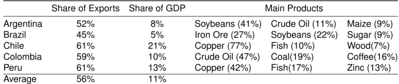
Table 1shows the commodity export profile for each country in the sample cal-culated as the arithmetic average from yearly SITC level 4 groups UN COMTRADE trade data from 1995-2015. The profile of the countries in the sample is similar. Com-modities represent nearly half of total exports. Energy is relevant only in Colombian commodity exports, while metals and agricultural products are the main exports of the rest of the sample. The major difference between these countries is the importance of commodities exports in total GDP, ranging from 5% in Brazil to 21% in Chile.
Table 1: Commodity exports by country
Share of Exports Share of GDP Main Products
Argentina 52% 8% Soybeans (41%) Crude Oil (11%) Maize (9%)
Brazil 45% 5% Iron Ore (27%) Soybeans (22%) Sugar (9%)
Chile 61% 21% Copper (77%) Fish (10%) Wood(7%)
Colombia 59% 10% Crude Oil (47%) Coal(19%) Coffee(16%)
Peru 61% 13% Copper (42%) Fish(17%) Zinc (13%)
Average 56% 11%
Figures in parenthesis are the share of the product in total commodity exports.
Real commodity export prices indexes for each country, illustrated in Figure1, were calculated as in Deaton and Miller (1996), Fernandez, Gonzalez and Rodriguez
(2015),Shousha(2016) following 4 steps:
1. Relate SITC level 4 groups and the IMF commodity prices database;
2. Find the value of each primary commodity exports using the UN COMTRADE database for each country, and take the average;
3. Weight each commodity by dividing its average share in exports for the sample period and compute a geometric weighted average of nominal commodity export prices;
4. Calculate the real commodity price index by dividing the nominal price index by the U.S. CPI.
Chapter 2. Data 15
Figure 1: Real Commodity Export Prices (1995 = 100)
Table 2 shows key business cycles statistics for the sample. The sign of the correlations are the same for all countries, but its magnitudes vary considerably. While real export commodity prices correlate positively with GDP and investment, it corre-lates negatively with country risk and this correlation is strong for all countries except Argentina and Chile. Country risk is also negatively correlated with GDP1. These
cor-relations are ad-hoc assumptions in the current business cycle literature which we propose to endogenize in our model.
Table 2: Business Cycles Statistics
Argentina Brazil Chile Colombia Peru Average
𝜎𝑌 3% 2% 2% 1% 2% 2% 𝜎𝐼 9% 5% 2% 6% 6% 6% 𝜌𝑃,𝑌 0.25 0.25 0.35 0.29 0.22 0.27 𝜌𝑃,𝐼 0.32 0.25 0.34 0.20 0.19 0.26 𝜌𝑃,𝑅 -0.11 -0.87 -0.23 -0.87 -0.93 -0.60 𝜌𝑌,𝑅 -0.39 -0.28 -0.30 -0.29 -0.19 -0.29 𝜌𝐼,𝑅 -0.38 -0.25 -0.30 -0.20 -0.16 -0.26 𝐵 𝑌 57% 67% 11% 39% 32% 41%
The letters 𝑌 , 𝐼, 𝑃 , 𝑅 are respectively: logs of GDP, investment, real commodity prices and EMBI+. 𝑌 and 𝐼 were detrended using HP filter with smoothing parameter of 1600 while R and P do not have trends. 𝜎𝑋is the standard deviation of variable 𝑋 and 𝜌𝑋,𝑍 is the correlation coefficient of variables 𝑋
and 𝑍.𝐵
𝑌 is the average debt-to-GDP ratio for each country.
We now present the model used to evaluate the importance of commodity price shocks and the country risk channel in business cycles.
1 Neumeyer and Perri(2005) show that this correlation is a standard feature of emerging economies,
16
3 The Model
The model consists of a small open economy producing a homogeneous good that can be consumed or invested and a continuum of risk-neutral international finan-cial intermediaries performing the role of international finanfinan-cial markets with access to a risk-free interest rate 𝑟*. The economy has a production function 𝑓 (𝑘) and a benevo-lent government who chooses consumption, investment, the amount of borrowing and to default or not on existing debt to maximize the utility of a continuum of identical consumers: 𝐸0 ∞ ∑︁ 𝑡=0 𝛽𝑡𝑢(𝑐) (3.1)
Where c denotes consumption good, 0 < 𝛽 < 1 the discount factor, and 𝑢 is the utility function satisfying the typical Inada conditions. For simplicity, we abstain to model commodities production and followFernandez, Gonzalez and Rodriguez(2015) where, in every period, the government may extract a fixed commodity endowment 𝑋. Although we could model commodity production, we prefer to assume an exogenous process for its prices reflecting the fact that domestic conditions of commodity produc-ing countries do not influence commodities prices. Moreover, commodities are mostly natural resources, therefore it is not only a matter of investing in the sector to increase production. The government sells its commodities for the price of 𝑝. We assume that 𝑝is exogenous and follows a first-order Markov process with finite support P and tran-sition matrix Π. We also assume an extraction cost 𝑝 to be paid by the sovereign. If in period 𝑡, 𝑝 < 𝑝, the government does not extract the commodity.
Let 𝑏 be the amount of debt held by the country at the beginning of each pe-riod. In normal times, the country repays all of its debt every period and can borrow from international markets for a price 𝑞. In equilibrium, 𝑞 will depend on the state of commodity prices 𝑝, capital and debt stocks 𝑘 and 𝑏. We denote the value function of the economy in normal states, when the country has access to financial markets, as 𝑉 (𝑝, 𝑘, 𝑏).
The sovereign decides to default or not at the beginning of each period. Let 𝑉𝑑𝑒𝑓 denote the value function of a country that chooses to default and 𝑉𝑝𝑎𝑦 the value
function of the country choosing to repay its debts. When default is optimal, 𝑉𝑑𝑒𝑓 >
𝑉𝑝𝑎𝑦 and the government does not pay its past debt. The country in default phase is
excluded from the international financial market and, thus, cannot borrow. Also, it faces another punishment of 𝛾% drop in commodity price while in autarky.
Chapter 3. The Model 17
Finally, the defaulting country is redeemed and re-enters a normal phase with probability 𝜑, when this happens all the past debt is forgiven, and the country has a zero debt stock. The sovereign chooses optimal policies 𝑏′ and 𝑘′ to maximize consumers’ utility. The expected value from next period onward and bond price 𝑞 incorporate the fact that the government could choose to default in the future. The sovereign has a lower bound on debt 𝑏′ ≥ 𝑧, not binding in equilibrium, to prevent Ponzi schemes.
The government problem in normal phase is:
𝑉 (𝑝, 𝑘, 𝑏) = max [𝑉𝑑𝑒𝑓(𝑝, 𝑘), 𝑉𝑝𝑎𝑦(𝑝, 𝑘, 𝑏)] (3.2) 𝑉𝑝𝑎𝑦 is given by: 𝑉𝑝𝑎𝑦(𝑝, 𝑘, 𝑏) = max 𝑏′,𝑘′ 𝑢(𝑐) + 𝛽𝐸[𝑉 (𝑝 ′ , 𝑘′, 𝑏′)] (3.3) s.t. 𝑐 + 𝑘′ + 𝑞(𝑝, 𝑘′, 𝑏′)𝑏′ ≤ 𝑓 (𝑘) + (1 − 𝛿)𝑘 + 𝑏 + max[𝑝 − 𝑝, 0]𝑋 (3.4) 𝑉𝑑𝑒𝑓 is given by: 𝑉𝑑𝑒𝑓(𝑝𝑡, 𝑘𝑡) = max 𝑘′ 𝑢(𝑐) + 𝛽𝐸[(1 − 𝜑)𝑉 𝑑𝑒𝑓(𝑝′ , 𝑘′) + 𝜑𝑉 (0, 𝑘′, 𝑝′)] (3.5) s.t. 𝑐 + 𝑘′ ≤ 𝑓 (𝑘) + (1 − 𝛿)𝑘 + max[(1 − 𝛾)𝑝 − 𝑝, 0]𝑋 (3.6) For a given capital and bond levels (𝑝, 𝑏) default is optimal for price levels pro-vided by the default set:
𝐷(𝑘, 𝑏) := {𝑝 : 𝑉𝑝𝑎𝑦(𝑝, 𝑘, 𝑏) < 𝑉𝑑𝑒𝑓(𝑝, 𝑘)} (3.7) When the government defaults, risk-neutral international lenders do not receive any repayment since we ignore the possibility of debt renegotiation1asArellano(2008)
does. The default function 𝑑(𝑝, 𝑘, 𝑏) = 1 if 𝑝 ∈ 𝐷(𝑘, 𝑏) and 0 otherwise. From a zero profit condition we must have:
𝑞(𝑝, 𝑘′, 𝑏′) = 1 − 𝐸[𝑑(𝑝
′, 𝑘′, 𝑏′)|𝑝])
1 + 𝑟* (3.8)
Chapter 3. The Model 18
Where 𝐸[𝑑(𝑝′, 𝑘′, 𝑏′)|𝑝]is the expected default probability. We define the country interest rate as the inverse of the debt price: ¯𝑟 = 1𝑞 − 1, country spread is, therefore, defined by the difference of country and risk-free interest rates: ¯𝑟 − 𝑟*.
With the equations above, we can define the model’s equilibrium:
Definition 1 Let 𝑠 = {𝑝, 𝑘, 𝑏} be the aggregate states for the economy. The recursive equilibrium for this economy is defined as a set of policy functions for (i) consumption 𝑐(𝑠); (ii) Sovereign bond holdings 𝑏′(𝑠); (iii) Sovereign capital stock 𝑘′(𝑠); and (iv) the bond price function 𝑞(𝑝, 𝑘′, 𝑏′)such that:
1. Taking as given the sovereign’s policies, households’ consumption 𝑐(𝑠) satisfies the resource constraint.
2. Taking as given the bond price function 𝑞(𝑝, 𝑘′, 𝑏′), the government’s policy func-tions and default sets 𝐷(𝑘, 𝑏) satisfies the sovereign problem.
3. Bond prices 𝑞(𝑝, 𝑘′, 𝑏′)reflect the sovereign’s default probabilities and are
consis-tent with international lenders’ expected zero profits.
Eaton and Gersovitz(1981),Arellano(2008) showed that in models with stochas-tic endowment the cardinality of the default set 𝐷(𝑘, 𝑏) is decreasing in 𝑏 since the value of repayment 𝑉𝑝𝑎𝑦 is increasing in 𝑏. Gordon and Guerrón-Quintana (2016)
ar-gues, quantitatively, that it is not possible to state how the cardinality of the default set changes with a variation of 𝑘 since the difference 𝑉𝑝𝑎𝑦 − 𝑉𝑑𝑒𝑓 varies in erratic ways for
different levels of 𝑏, the same relation is present in this model. We show quantitatively, for our calibration, that if a country default at a given price it would also choose to default if price levels were lower and capital and debt stocks were the same.
We now proceed with the strategy used for the estimation of 𝑝, the calibration of the parameters and to solve the model numerically.
19
4 Calibration and Solution Strategy
4.1
Calibration
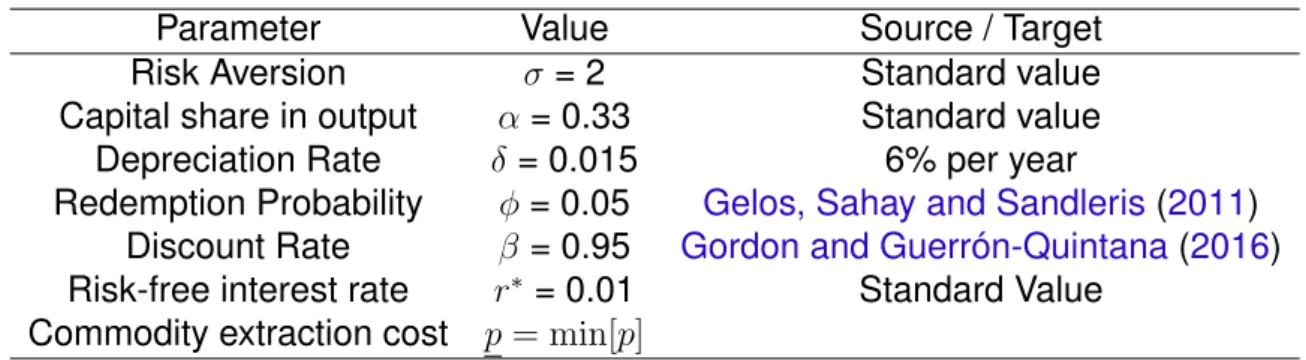
We calibrate the model following the sovereign default literature to assess the effect of commodity prices fluctuations on country risk and business cycles. Each pe-riod corresponds to a quarter. Utility function is set as standard CRRA of the form 𝑢(𝑐) = 𝑐1−𝜎1−𝜎−1 with risk-aversion parameter 𝜎 = 2 as is common in the literature. Pro-duction function is a standard normalized Cobb-Douglas 𝑓 (𝑘) = 𝑘𝛼. The capital share
in output, 𝛼, is set at 0.33. The standard depreciation rate in the literature for emerging economies is 6% per year, translating into a 𝛿 at 0.015 in our quarterly model. The probability of return to financial markets, 𝜑, is set at 0.05 following Gelos, Sahay and Sandleris(2011), who documents that countries stay, on average, five years in autarky following a default.
Table 3: Calibrated Parameters Value
Parameter Value Source / Target
Risk Aversion 𝜎= 2 Standard value
Capital share in output 𝛼= 0.33 Standard value Depreciation Rate 𝛿 = 0.015 6% per year
Redemption Probability 𝜑 = 0.05 Gelos, Sahay and Sandleris(2011) Discount Rate 𝛽 = 0.95 Gordon and Guerrón-Quintana(2016) Risk-free interest rate 𝑟* = 0.01 Standard Value
Commodity extraction cost 𝑝 = min[𝑝]
Sovereign default models usually require an unrealistically low discount rates, 𝛽, to match data moments such as debt-to-GDP ratio and default rates. In our model, a low beta is not able to replicate the relation of prices and risk observed in the data. We thus follow another approach, setting 𝛽 = 0.95 as found by Gordon and Guerrón-Quintana(2016)1. Extraction cost 𝑝 was set to the lowest possible value of 𝑝, explained
below, so that only in extreme case the sovereign does not receive any resources from commodities, this cost aims to capture the fact that at low prices commodity extraction might not be profitable. Table 3summarizes the fixed parameters.
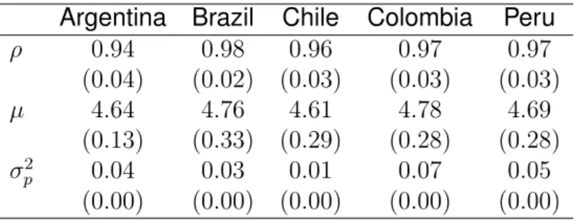
Commodity prices 𝑝 were assumed to follow an AR(1) process of the form:
log(𝑝𝑡+1) = (1 − 𝜌)𝜇 + 𝜌 log(𝑝𝑡) + 𝜖 (4.1)
1 For having 𝛽 = 0.95 Gordon and Guerrón-Quintana (2016) includes long-term debt and capital
Chapter 4. Calibration and Solution Strategy 20
The autocorrelation coefficient, 𝜌, the long run average log of the price 𝜇 and the i.i.d. shock 𝜖 ∼ 𝑁 (0, 𝜎2
𝑝) were estimated for each of the countries in the sample
and the estimation results are in table4. Since the estimated value were similar for all countries and shocks are highly persistent, we chose to run the model with the Chilean values of 𝜌 = 0.96, 𝜇 = 4.61 and 𝜎𝑝 = 0.01.
Table 4: Estimation Results
Argentina Brazil Chile Colombia Peru
𝜌 0.94 0.98 0.96 0.97 0.97 (0.04) (0.02) (0.03) (0.03) (0.03) 𝜇 4.64 4.76 4.61 4.78 4.69 (0.13) (0.33) (0.29) (0.28) (0.28) 𝜎𝑝2 0.04 0.03 0.01 0.07 0.05 (0.00) (0.00) (0.00) (0.00) (0.00)
All coefficients are significant at 0.01 confidence level. Figures in parenthesis are standard errors.
There are two parameters, the exogenous commodity endowment 𝑋 and de-fault punishment 𝛾, which were set to match two empirical data moments: commodities-to-GDP and debt-commodities-to-GDP ratios. We present these parameters with the results in the next section.
4.2
Solution Strategy
We solve the model by the discrete state-space method. We approximate the estimated commodity prices AR(1) by a Markov-chain following Kopecky and Suen
(2010) method for a highly persistent process using 60 grid points. The asset and capital spaces are discretized in 50 and 80 points, respectively2. Capital and debt
limits were set as never being binding in equilibrium. The solution algorithm is based onAguiar and Gopinath (2006) and consists of:
1. Assume an initial price function 𝑞0(𝑝, 𝑘′, 𝑏′) = 1+𝑟1*∀(𝑝, 𝑘′, 𝑏′).
2. Guess initial 𝑉0𝑑𝑒𝑓and 𝑉 𝑝𝑎𝑦
0 and use 𝑞0to iterate until convergence of the bellmans
equations3.3and3.5.
3. With the new Value Functions, find 𝑉 (𝑝, 𝑘, 𝑏) = max [𝑉𝑑𝑒𝑓(𝑝, 𝑘), 𝑉𝑝𝑎𝑦(𝑝, 𝑘, 𝑏)], the
optimal policy functions and the default set 𝐷(𝑘′, 𝑏′).
2 Due to lack of computational power, we were not able to use more grid points but some tests were
made, and the model is stable with this grid size. We are looking forward to run the model on a better computer.
Chapter 4. Calibration and Solution Strategy 21
4. Finally, update the price 𝑞1(𝑝, 𝑘′, 𝑏′) = 1−𝐸[𝑑(𝑝 ′,𝑘′,𝑏′)|𝑝]
1+𝑟* and use it to iterate steps 2
22
5 Results
We begin this section by matching the baseline model to Chilean data and an-alyzing the behavior of the model economy. We proceed by calculating how much of the output fluctuation are due to commodity price volatility muting the investment chan-nel. Then, we propose the following experiments with the model: run one version for a highly indebted country, other with lower commodity-to-GDP ratio and finally a version with low commodity and high debt. We end this section presenting, numerically, the default sets and debt prices.
In the baseline model, the parameters 𝑋, the commodity endowment, and 𝛾, the default cost, were set to match two moments of Chilean data, Commodity-to-GDP and Debt-to-GDP ratios. At higher levels of 𝛾, the economy can sustain more debt in equilibrium since lenders know that the government will only choose to incur default costs in extreme situations. A default cost, 𝛾 of 4.5% is required to match Chilean data. This figure is close to the ones estimated by Martinez and Sandleris (2011), Rose
(2005) who found, respectively, a decline in trade of approximately 3.2% and 8% per year.
First, we analyze the implications of capital accumulation in the model. Figure2
plots the bond price schedule, with commodity price at its mean value, along with capital and debt levels dimensions. For a given capital value, we observe higher bond prices (low q) at higher levels of debt. This figures also shows us an interesting relation: additional capital can sustain higher debt levels, but not in a monotonic way.
To understand this relation, figure3plots how the difference between 𝑉𝑝𝑎𝑦(𝑝, 𝑘, 𝑏)
and 𝑉𝑑𝑒𝑓(𝑝, 𝑘) evolves with capital stock (right figure) and for different debt levels (left
figure). When indebtedness is high, the value of autarky increases in capital slower than repayment value. Therefore, 𝑉𝑝𝑎𝑦(𝑝, 𝑘, 𝑏) − 𝑉𝑑𝑒𝑓(𝑝, 𝑘)is increasing in capital stock
and the relation is inverted at low debt levels.
Gordon and Guerrón-Quintana(2016) presents an elaborated discussion of why this happens, but the key is to understand that when indebted, additional capital bene-fits the government by augmenting its output and reducing debt costs. While additional capital only benefits a government in autarky through the output channel. When debt is not costly (i.e. 𝑞 is close to risk-free levels), at high 𝑘 or low 𝑏 states, the second benefit of capital vanishes and is the sovereign in autarky who enjoys more of capital at higher levels. Since capital stocks increase output and, jointly with the benefit of not having to repay debt, default punishments are outweighed.
Chapter 5. Results 23
Figure 2: Bond prices with average commodity price
Figure 3: 𝑉𝑝𝑎𝑦(𝑝, 𝑘, 𝑏) − 𝑉𝑑𝑒𝑓(𝑝, 𝑘)
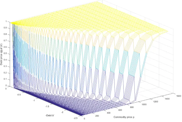
prices dimensions with capital fixed in its median grid value. This figure reveals that higher prices can sustain higher debt levels.
Chapter 5. Results 24
Figure 4: Bond prices with median capital
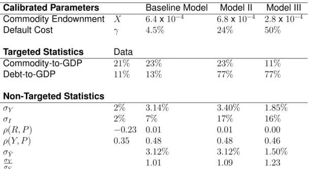
Table 5presents the results of the model. GDP volatility of the baseline model at 3.14% is reasonably close to the figure observed in Chilean data of 2% taking into account that the model’s volatility reflects mainly commodity prices volatility, which is the same as the estimated values for the Chilean economy. As expected, investment volatility is much higher than observed in data since after a negative price shock, to smooth consumption the sovereign chooses to reduce investment instead of borrowing in financial markets because the cost of debt is higher when prices are low.
The model is not able to replicate correlation between commodities prices and country risk1. When commodity prices are high, the model economy invests and
accu-mulate more debt increasing GDP and spreads. However, when prices are high, the economy have more resources to repay its debt and spread also tends to be lower. In our calibration, no effect is dominant, and correlations are nearly zero. When com-modity prices change dramatically from a high level to a low level, the economy has incentives to default on its debt instead of reducing its capital. Recall that in our model there are no productivity shocks as is common in standard RBC models. Thus, capi-tal’s marginal productivity does not change in better states of the world and investment
1 Gordon and Guerrón-Quintana(2016) includes capital adjustment costs and long-term debt to match
Chapter 5. Results 25
Table 5: Results
Calibrated Parameters Baseline Model Model II Model III Commodity Endownment 𝑋 6.4x 10⁻⁴ 6.8 x 10⁻⁴ 2.8 x 10⁻⁴
Default Cost 𝛾 4.5% 24% 50%
Targeted Statistics Data
Commodity-to-GDP 21% 23% 23% 11% Debt-to-GDP 11% 13% 77% 77% Non-Targeted Statistics 𝜎𝑌 2% 3.14% 3.40% 1.85% 𝜎𝐼 2% 7% 17% 16% 𝜌(𝑅, 𝑃 ) −0.23 0.01 0.01 0.00 𝜌(𝑌, 𝑃 ) 0.35 0.48 0.48 0.46 𝜎𝑌¯ 3.12% 3.12% 1.50% 𝜎𝑌 𝜎𝑌¯ 1.01 1.09 1.23
The Baseline model was calibrated to match Chilean data. Model II is a highly indebted country with high commodity-to-GDP ratio. Model III is a highly indebted country low high commodity-to-GDP ratio.
¯
𝑌 is the GDP when capital is constant.
is not sacrificed in lower states.
Using this model as a laboratory, we intend to verify if the country risk channel can amplify the economy’s volatility in response to commodity prices fluctuations. To do so, we remove investment of the economy by fixing the capital level at the economy’s average value. In this world, all the volatility comes from the mechanical channel of commodity prices. We find that the volatility of the full model is only 1.01 times higher than the one with fixed capital. This low amplification effect contradicts what was found by Shousha (2016), Fernandez, Gonzalez and Rodriguez (2015) where the interest rate channel was the primary driver of commodity shocks.
This might be happening because in our calibration debt levels are low com-pared to most of the emerging economies even though the commodity share of GDP is high. To verify if countries with different indebtedness or commodity shares would behave differently, we calibrate two other versions of the model. Model II has high commodity and debt shares of GDP and Model III has low commodity and high indebt-edness.
Models II and III uses the same parameters as the baseline model. The only difference is in the default cost 𝛾 and the commodity endowment 𝑋. To achieve a ratio of commodity-to-GDP of 77% models II and III requires a reduction of 24% and 50%, respectively, in commodity prices as default punishment 𝛾. These default costs seem too high compared to the data, but we do no expect that all the punishment in trade suffered by countries with low commodity share in GDP comes from a reduction
Chapter 5. Results 26
in commodity prices. Such reduction might be interpreted as a reduced form of other punishments suffered by those countries.
The results for model II and III are similar to those of our baseline version. Naturally, GDP volatility of model III is lower than the baseline due to the mechanical effect of commodities. Both models present a considerably higher investment volatility. This happens because the greater default cost lowers its incentives to default and the economy will acquire more debt in equilibrium. More debt means that the government can invest more during good times, but this also means that it can sacrifice more capital stock to smooth consumption instead of increasing its debt stocks.
The most interesting difference between the models is when we compare the volatility of GDP in steady state with the volatility of the full model. Both models now present a significant amplification due to the country risk channel. Model II has an amplification of 1.09 while model III is at 1.23 times its volatility in steady state. Thus, in our setup, the risk channel is more important for a highly indebted country. This was not unexpected since a country dependent on external finance would suffer more from interest rate shocks than one with lower debt.
Perhaps surprisingly, this effect is higher if the country is less dependent on commodities. In our setup, the commodity sector acts as an anchor of GDP’s fluctu-ation. When the country has a low commodity endowment, it must rely mostly on its internal sector which for consumption smoothing. The internal sector, in turns, depends on investment and interest rates. The endogenous default framework implies that in good states, debt is cheap and the sovereign invests and even when commodities are only a small fraction of the output, this effect can lead to high volatility in interest rates. An implication of this model is that in countries such as Brazil and Argentina the risk channel is relatively larger than it is to Chile. This is not only due to the high indebt-edness of these countries when compared to Chile, but also because their economy is less dependent on commodities and are, therefore, more vulnerable to interest rates shocks. Following a commodity price meltdown, we should expect a higher response of Brazilian and Argentinean interest and investment rates than to Chile. Even though, in absolute values, the recession in the Chilean economy could be more severe.
27
6 Conclusion
Recent models investigate the effects of commodity prices fluctuation in the business cycle and find that the country risk channel is one of the most important drivers of the effect. However, these models assume an exogenous response of coun-try risk to commodity prices. This paper provided a simple micro-founded framework to endogenize this relation based on the sovereign default literature. We modify the standard endogenous default model by including an endogenous production function and an exogenous commodity endowment.
Our model can explain how country-risk amplifies commodity prices volatility effect on GDP’s fluctuation. When commodity prices are low, default risk increases the cost of new debt issuance. When debt is costly, the government reduces investment and, therefore, reduces production in the next periods. In the model, default happens when the country is highly indebted and there is a dramatic change in commodity prices as was documented in previous empirical works.
From a quantitative perspective, our model can assess the importance of the country-risk amplification channel. For our baseline economy, which mimics Chilean data, the channel does not seem to play an important role. However, this is not a surprise since Chilean indebtedness level is much lower than the indebtedness level of other emerging economies. When the model replicates a more indebted economy, we find that the country-risk channel amplifies commodity prices volatility effect on GDP by 1.23 times. This effect is more relevant for countries depending less on commodities such as Brazil or Argentina.
This paper also followed a standard methodology to calculate a new commodity prices index for five Latin-American countries. The index was used to estimate the stochastic process followed by commodity prices in the model.
This work could be extended in several fashions. First, commodity production could also be endogenized to explain better how the mechanisms work. Second, one could investigate the effects of long-term debt in the model since it is known that default models with capital investment perform better when long-term debt is allowedguerron. Third, the commodity prices index could be used to investigate better how commodity prices influence other aspects of emerging economies.
28
Bibliography
AGUIAR, M.; GOPINATH, G. Defaultable debt, interest rates and the current account. Journal of International Economics, v. 69, n. 1, p. 64–83, June 2006. Cited on page
20.
ARELLANO, C. Default Risk and Income Fluctuations in Emerging Economies. American Economic Review, v. 98, n. 3, p. 690–712, June 2008. Cited 6 times on pages7,8,10,12,17, and18.
BAI, Y.; ZHANG, J. Duration of sovereign debt renegotiation. Journal of International Economics, v. 86, n. 2, p. 252–268, 2012. Cited on page 17.
BAI, Y.; ZHANG, J. Financial integration and international risk sharing. Journal of International Economics, v. 86, n. 1, p. 17–32, 2012. Cited on page12.
BULOW, J.; ROGOFF, K. Sovereign Debt: Is to Forgive to Forget? American Economic Review, v. 79, n. 1, p. 43–50, March 1989. Cited on page12.
DEATON, A.; MILLER, R. International Commodity Prices, Macroeconomic
Performance and Politics in Sub-Saharan Africa. Journal of African Economies, v. 5, n. 3, p. 99–191, October 1996. Cited on page 14.
EATON, J.; GERSOVITZ, M. Debt with Potential Repudiation: Theoretical and Empirical Analysis. Review of Economic Studies, v. 48, n. 2, p. 289–309, 1981. Cited 3 times on pages10,12, and18.
FERNANDEZ, A.; GONZALEZ, A.; RODRIGUEZ, D. Sharing a Ride on the Commodities Roller Coaster; Common Factors in Business Cycles of Emerging Economies. [S.l.], 2015. Cited 4 times on pages 12,14,16, and25.
FERNáNDEZ, A.; SCHMITT-GROHé, S.; URIBE, M. World Shocks, World Prices, and Business Cycles: An Empirical Investigation. In: NBER International Seminar on Macroeconomics 2016. [S.l.]: National Bureau of Economic Research, Inc, 2016, (NBER Chapters). Cited on page11.
GELOS, R. G.; SAHAY, R.; SANDLERIS, G. Sovereign borrowing by developing countries: What determines market access? Journal of International Economics, v. 83, n. 2, p. 243–254, March 2011. Cited on page19.
GORDON, G.; GUERRóN-QUINTANA, P. Dynamics of investment, debt, and default. [S.l.], 2016. Cited 5 times on pages12,18,19,22, and24.
HILSCHER, J.; NOSBUSCH, Y. Determinants of Sovereign Risk: Macroeconomic Fundamentals and the Pricing of Sovereign Debt. Review of Finance, v. 14, n. 2, p. 235–262, 2010. Cited on page 12.
KOPECKY, K.; SUEN, R. Finite State Markov-chain Approximations to Highly Persistent Processes. Review of Economic Dynamics, v. 13, n. 3, p. 701–714, July 2010. Cited on page 20.
Bibliography 29
KOSE, M. A. Explaining business cycles in small open economies: ’How much do world prices matter?’. Journal of International Economics, v. 56, n. 2, p. 299–327, March 2002. Cited on page 11.
MARTINEZ, J. V.; SANDLERIS, G. Is it punishment? Sovereign defaults and the decline in trade. Journal of International Money and Finance, v. 30, n. 6, p. 909–930, October 2011. Cited 2 times on pages12and22.
MENDOZA, E. G. The Terms of Trade, the Real Exchange Rate, and Economic Fluctuations. International Economic Review, v. 36, n. 1, p. 101–37, February 1995. Cited on page11.
NEUMEYER, P. A.; PERRI, F. Business cycles in emerging economies: the role of interest rates. Journal of Monetary Economics, v. 52, n. 2, p. 345–380, March 2005. Cited 2 times on pages 12and15.
REINHART, C. M.; REINHART, V.; TREBESCH, C. Global Cycles: Capital Flows, Commodities, and Sovereign Defaults, 1815-2015. American Economic Review, v. 106, n. 5, p. 574–580, May 2016. Cited on page 12.
ROSE, A. K. One reason countries pay their debts: renegotiation and international trade. Journal of Development Economics, v. 77, n. 1, p. 189–206, June 2005. Cited 2 times on pages13and22.
SHOUSHA, S. Macroeconomic effects of commodity booms and busts: The role of financial frictions. Working Paper, 2016. Cited 3 times on pages 12,14, and25. YUE, V. Z. Sovereign default and debt renegotiation. Journal of International Economics, v. 80, n. 2, p. 176–187, March 2010. Cited on page 17.