A COMPARISON ABOUT THE PREDICTIVE ABILITY OF
FCGARCH, FACING EGARCH AND GJR
Ricardo Miguel Borges Matias
Project submitted as partial requirement for the conferral of
Master in Finance
Supervisor:
Prof. Dr. José Dias Curto, Associate Professor, ISCTE-IUL Business School, Quantitative Methods Department
Co-Supervisor
Dr. Renato Costa, Lecturer, Western Institute of Technology at Taranaki (WITT), Engineering Department
Abstract
In order to study the volatility of a stock market, several volatility models have been created, studied and improved throughout the time. Due to the extreme and actual situation in international stock market’s volatility, the main objective of this thesis is to focus on the FCGARCH model created by Medeiros and Veiga (2009), and compare it with some of the most popular asymmetric autoregressive conditional heteroskedasticity models, such as EGARCH and GJR.
Using the daily returns of 5 most important international stock market indexes, such as S&P500 (USA), FTSE100 (UK), Nikkei225 (Japan), DAX30 (Germany) and PSI20 (Portugal), and using the Harvey-Newbold test, we are going to check which of these models is the best one to fit the conditional heteroskedastic volatilities of the returns of the indexes under study.
In order to make the thesis possible, I have created the FCGARCH, EGARCH and GJR models’ codes in Matlab, with the help of my co-supervisor, Doctor Renato Costa, as well as used the Harvey-Newbold test in E-views, created by my supervisor, Professor José Dias Curto.
According to the estimation results, in the in-sample analysis, when looking at the Quasi-Maximum-Log likelihood goodness-of-fit measure, the FCGARCH fits most of the indexes’ returns under study, where, in the out-of-sample analysis, according to the Harvey-Newbold test for multiple forecasts encompassing, the results show that the GJR seems to encompass the other two models in most of the indexes, thus concluding that GJR seems to be the best model to forecast the volatility.
Keywords: Forecasting volatility, EGARCH, GJR, FCGARCH
Resumo
Para que possamos estudar a volatilidade de uma ação, muitos foram os modelos criados, estudados e melhorados ao longo do tempo. Devido à extrema e atual situação da volatilidade nos mercados acionistas internacionais, o principal objetivo desta tese é focar no modelo FCGARCH, criado por Medeiros e Veiga (2009), e compará-lo com alguns dos mais importantes modelos heterocedásticos, autorregressivos e assimétricos, como o EGARCH e o GJR.
Utilizando os retornos diários de 5 dos índices mais importantes a nível internacional, tais como S&P500 (EUA), FTSE100 (RU), Nikkei225 (Japão), DAX30 (Alemanha) e PSI20 (Portugal), e usando o teste de Harvey-Newbold, vamos descobrir qual dos modelos apresentados é o que melhor descreve o comportamento das variâncias condicionais heterocedásticas dos retornos dos índices sob estudo.
Para que a criação desta tese fosse possível, tive de criar os códigos dos modelos do FCGARCH, EGARCH e GJR no Matlab, com a ajuda do meu co-orientador, o Doutor Renato Costa, assim como usar o teste de Harvey-Newbold no E-views, criado pelo meu orientador, o Professor José Dias Curto.
De acordo com os resultados estimados, na análise in-sample, ao olharmos para a medida de quase-máxima-verosimilhança, o FCGARCH descreve bem a maioria dos retornos sob estudo, enquanto, na análise out-of-sample, de acordo com o teste de Harvey-Newbold para a abrangência de previsões, os resultados demonstram que o GJR parece abranger os outros dois modelos na maioria dos índices, desta forma concluindo que o GJR parece ser o melhor modelo para prever a volatilidade.
Palavras-chave: Previsão de volatilidade, EGARCH, GJR, FCGARCH
Acknowledgements
Since, with this thesis, I am going to reach a new goal, not only professionally but also in life as well, I would like to thank all the people who helped me throughout this process.
First of all, I would like to thank my friends and the Tuna Académica do ISCTE, for the company, partying and understanding given in these years, which helped me developing my skills, not only in a professional way, but also in a personal way.
I would like to thank also Doctor João Ribeiro and his assistant, Elisabete Faria, for the time and help given in order to finish this thesis in time, as well as the professional and personal development I accomplished through this months since I started working in Mercal.
Furthermore, I would like to thank my co-supervisor, Doctor Renato Costa for all the collaboration, not only for the creation of the Matlab codes, but also for the help and support he had given me through the elaboration of this thesis and the codes related to FCGARCH. Without his insights, this thesis wouldn’t have the same quality as it has now.
I also would like to thank my supervisor, Professor José Dias Curto, for the kind support, guidance and insight in helping me to structure this thesis, as well as to improve the quality of the thesis with the introduction of the Harvey-Newbold test and its codes created by him.
Last but definitely not least, I would like to thank my parents and sister who supported me during all of these years of studies, not only financially, but also emotionally. Having the patience and understanding needed to a person like me. I hope and will try that all of their work with me and my life will not be in vain.
I
Index
1. Introduction ... 1
2. Models under Comparison – EGARCH, GJR and FCGARCH... 4
3. Empirical Study ... 10
3.1. Statistical Properties of Returns ... 10
3.2. In-sample Analysis ... 11
3.2.1. Descriptive Statistics ... 11
3.2.2. Estimation Results ... 12
3.3. Out-of-sample Analysis - Results ... 18
4. Conclusions ... 21
References ... 23
Annexes ... 25
1.1. Daily Closing Prices and Returns of the assets ... 25
1.2. Matlab Codes ... 26
1.2.1. Estimation of Parameters ... 26
1.2.2. Forecasting Returns ... 30
1.3. E-views Codes ... 31
II
Executive Summary
Due to the financial instability faced nowadays throughout the world, the need of the existence of a plausible study of the volatility in the international stock market’s volatility has been the main point of interest among the academy, the industries, and the markets themselves.
In this thesis, we are going to focus on the models which have reached a consensus on being the most important ones for the study of the volatility, starting with the ARCH model by Engle (1982), and continuing with other models such as GARCH by Bollerslev (1986), EGARCH by Nelson (1991), GJR by Glosten, Jagannathan and Runkle (1993), and STGARCH by Hagerud (1997).
However, the focus for this thesis will be on the model proposed by Medeiros and Veiga (2009), the FCGARCH model, which, among others, has as a main advantage the fact that the model can deal with more than 2 regimes, while others cannot.
Thus, this thesis will be focused on the comparison of the FCGARCH model, with other two main important models, the EGARCH and the GJR models. Creating the codes in Matlab for the estimation of the parameters for these models, and using the Harvey-Newbold test code on E-views, we will try to conclude which of these three models seems to be the best one to predict the volatilities of the assets.
Using the S&P500 (USA), FTSE100 (UK), Nikkei225 (Japan), DAX30 (Germany) and PSI20 (Portugal) indexes’ returns from January 2001 to December 2011, I divided the sample in two main periods, being the first 2/3 of the observations used for the parameters estimation (In-sample analysis), where, using these results, the final 1/3 are considered as the forecast period (Out-of-sample Analysis).
According to the estimation in-sample results, the Quasi-Maximum-Likelihood shows that the FCGARCH model seems to be the best model in most of the indexes, fitting the dynamics of the returns of the indexes in study. If we consider other goodness-of-fit measures, such as Akaike and Schwarz criterions, although the FCGARCH model has a significant number of parameters, the results confirm the QML conclusions, favoring not only the FCGARCH model, but also the GJR model.
III
The out-of-sample results, based on the Harvey-Newbold encompassing test, show that the best model to predict the volatility forecasts for the majority of the indexes under study, seems to be, not the FCGARCH model, but the GJR model.
This thesis and its empirical result tends to be useful for those who want, not only to get deeper in the FCGARCH model, but also to be closer to find the best model, regarding the forecast of volatility in financial markets, mainly during periods of high volatility.
IV
Sumário Executivo
Devido à instabilidade económica enfrentada a nível mundial ao longo dos tempos, a necessidade na existência de um estudo plausível da volatilidade nos mercados internacionais acionistas tem vindo a ser o maior ponto de interesse entre a academia, as empresas, e os próprios mercados.
Nesta tese, iremos focar-nos nos modelos aos quais chegou-se a um consenso relativamente a serem os mais importantes a serem estudados para a volatilidade, começando com o modelo ARCH de Engle (1982), e continuando com outros modelos, tais como GARCH de Bollerslev (1986), EGARCH de Nelson (1991), GJR de Glosten, Jagannathan e Runkle (1993), e STGARCH de Hagerud (1997).
No entanto, o foco nesta tese será no modelo proposto por Medeiros e Veiga (2009), o modelo FCGARCH, sendo que, entre outros, tem a principal vantagem de poder lidar com mais do que dois regimes, algo que os outros modelos não conseguem.
Sendo assim, esta tese focar-se-á na comparação entre o modelo FCGARCH, com outros dois principais modelos, o EGARCH e o GJR. Criando os códigos em Matlab para a estimação dos parâmetros para estes modelos, e usando o código do teste de Harvey-Newbold no E-views, vamos tentar concluir quais destes três modelos parece ser o melhor para prever as volatilidades das ações.
Usando os retornos dos índices S&P500 (EUA), FTSE100 (RU), Nikkei225 (Japão), DAX30 (Alemanha) e PSI20 (Portugal), desde Janeiro de 2001 até Dezembro de 2011, dividi a amostra em dois períodos distintos, sendo os primeiros 2/3 das observações usados para a estimação dos parâmetros (análise in-sample), donde, usando esses retornos, o 1/3 final será considerado o período de previsão (análise out-of-sample).
De acordo com os resultados da estimação in-sample, o indicador de Quase-Máxima-Verosimilhança demonstra que o modelo FCGARCH parece ser o melhor, na maioria dos índices, enquadrando-se nas dinâmicas dos retornos dos índices estudados. Se considerarmos outras medidas como os critérios de Akaike and Schwarz, apesar de o modelo FCGARCH apresentar um número significativo de parâmetros, os resultados confirmam as conclusões do QMV, favorecendo não só o FCGARCH como também o GJR.
V
Os resultados out-of-sample, baseados no teste de Harvey-Newbold, demonstram que o melhor modelo para prever a volatilidade na maioria dos índices, parece ser, não o modelo FCGARCH, mas sim o GJR.
Esta tese e seu resultado empírico tornam-se necessários para aqueles que querem não só aprofundar o modelo FCGARCH, mas também para estar mais próximo de encontrar o melhor modelo, relativamente à previsão da volatilidade nos mercados financeiros, principalmente durante períodos de elevada volatilidade.
1
1. Introduction
When we talk about stock markets, one of the first things that comes in our mind is volatility. Starting with Bachelier (1990), who identified an impossibility to predict stock returns, due to the huge number of factors that should be included in their forecast, this definition has been developed throughout the years, even more when the concept of market risk (uncertainty about the future market price of a financial asset) has been the main point of interest among the academy, the industries, and the markets themselves.
Nowadays, due to the development of technology and the fastness of how the information is passed throughout the world, we have an infinite number of arriving news which has a huge impact on the prices of stocks in the capital markets. Consequently, we are facing financial markets whose prices and returns change by the second, thus making even more difficult to predict how these markets are going to act in the recent future, and how these acts will affect their prices and returns in the future.
This uncertainty changed some of the minds and behaviors of the investors, who are considered more risk averse (want to invest and have the highest return at the minimum risk possible), and thus are more concerned about the variability of the returns of these markets.
Many authors tried to identify some regularity in the asset returns. Mandelbrot (1963: 418) concluded that “large changes tend to be followed by large changes, of either sign, and small changes tend to be followed by small changes”, thus describing the “volatility clustering effect”, in which we can conclude that the returns cannot be independent and identically distributed (i.i.d.). Black (1976) discovered the “Leverage effect”, a tendency for negative correlations between changes in the stock prices and in the volatilities of those prices, that is, unexpected bad news or negative innovations have a higher impact on the risk and the prices of a stock than positive news with the same magnitude.
On the same article, Black also discovered that there may be a co-movement among volatilities, saying that high volatility stocks are somewhat more correlated to market volatility changes rather than low volatility changes. Finally, Schwert (1989) found that during financial crisis and recessions, the volatility of the stock rises, but its relation with macroeconomic uncertainty is very weak, which means that maybe stock values are not that closely tied to the health of the economy as we should expect.
2
All these factors lead to one conclusion: We have to find a model which can predict the risk of certain stocks, always having in mind their regularities. Although this is difficult to find, some authors have reached some helpful models. However, each model has its own disadvantage: there is not a perfect model, so there is a continuous research for the perfect model.
In the last years several models have been proposed to deal with the stock markets’ volatility. Starting with the ARCH Model by Engle (1982), and continuing with other models such as GARCH by Bollerslev (1986), EGARCH by Nelson (1991), GJR by Glosten, Jagannathan and Runkle (1993), STGARCH by Hagerud (1997), among many others, we finally reach the FCGARCH model, proposed by Medeiros and Veiga (2009). It is to note the importance of FCGARCH, due to the fact that the model can deal with more than 2 regimes, while EGARCH and GJR can only deal with no more than 2 regimes, thus being FCGARCH a possible solution for the predictability of certain financial assets’ volatilities.
There are some researches and studies using FCGARCH which have already been made, such as the one made by Hillebrand and Medeiros (2008), which studied the statistical consequences of neglecting structural breaks and regime switches in autoregressive and GARCH models, proposing the FCGARCH model as a solution for the problem, since the regime-switches are governed by an observable variable, thus concluding that the FCGARCH is a variation of the GARCH model which contains and identifies the different volatility regimes. Another paper worth of mentioning is the one made by Costa (2010). He investigated the pricing of options according to the use of the FCGARCH model, making simulations according to the results estimated in Medeiros and Veiga’s paper. Finally, Salgado (2011) tested the predictive accuracy of some GARCH models, including the FCGARCH, concluding that the model has the best performance on realized volatility.
Based on this, the main purpose of this paper is to confirm the importance of the FCGARCH model, computing the predictability of three GARCH type models, mainly EGARCH, GJR and FCGARCH, according to the daily returns of 5 most important international stock market indexes, such as S&P 500 (USA), FTSE 100 (UK), DAX 30 (Germany), Nikkei 225 (Japan), and PSI 20 (Portugal).
In order to analyze the models and their characteristics according to the indexes in study, and with the help of my co-supervisor, Professor Renato Costa, I had to create the code for the programs for the estimation of the models in Matlab, not only for FCGARCH, but also
3
for EGARCH and GJR, so that each model can be compared in-sample according to the Quasi-Maximum-Log-likelihood. It is to note the complexity of these models, specially the FCGARCH, even more due to the fact that this model is very recent, and so there are very few studies talking about this model, as well as there are no codes shared to the public, thus obligating to create the codes from scratch, based on the paper from the creators Medeiros and Veiga (2009). These codes turn out to be crucial for the analysis in this thesis.
Although it was very challenging, I have been successful in this task, even more since the parameters estimated in this thesis follow all the constraints specified in the model and present in the codes. Consequently, for the out-of-sample analysis, I had to use the Harvey-Newbold test. In order to make some conclusions for this test, I used the code in E-views created by my supervisor, Professor José Dias Curto, which allowed me to make a better conclusion regarding the predicting capability of these three models.
The structure of this thesis is based on the following: first, we are going to make a small introduction and recap of the models in study, indicating their importance in the financial market and their main advantages and disadvantages, with a main focus on the FCGARCH model. Then, we are going to describe and analyze the data which we will use in this thesis, followed by the estimation results of the models’ parameters based on the same data, and make a comparison of the out-of-sample evaluation results, with the consequent discussion of the results. Finally, some conclusion remarks will be made.
4
2. Models under Comparison – EGARCH, GJR and FCGARCH
According to Majmudar and Benerjee (2004), financial volatility can be divided in three main groups: realized volatility, which is based on the standard deviation of the returns of the asset; implied/market volatility, representing the market prediction about future price fluctuations; and model volatility, based on theoretical models such as GARCH (Generalized Autoregressive Conditional Heteroskedasticity) and stochastic volatility. Since in this thesis we are focusing on the FCGARCH model, our main concern will be concentrated on this last category.
Let represent the price of one specific asset at time t. Using the logarithm return,
. (1) Let represent all the available information at time t-1, and . If we consider a constant volatility, then the returns at time t should be viewed as:
(2)
What happens with this formula is that although we are using a conditional mean, a constant volatility is not the best assumption to make. There is a volatility clustering effect studied by Mandelbrot (1963) and Fama (1965), which means that we have to assume since then that the volatility does change through time, and consequently, the variance must be heteroskedastic. This means that we have to assume that is now a stochastic process, and the conditional variance is denoted by .
In order to solve this problem, Engle (1982) tried an ARCH (Autoregressive Conditional Heteroskedasticity) model. In this model, we assume that the conditional variance is a linear function of the past q squared innovations, this is:
(3)
It is to note that in this model, , and , , so that the conditional mean and variance can be positive, and , to ensure that this process is covariance stationary. This model has the advantage of being easy to use, due to its simplicity of formulation and estimation, allowing also the impact of volatility clustering.
5
However, the ARCH model has many drawbacks, being the main one the fact that only affects the current volatility, which may be unrealistic, since the latter may respond differently to good or bad news ( or ), and the impact of a large shock only lasts for q periods, with a long length implying a large number of parameters, thus being more difficult to estimate.
Bollerslev (1986) tried to circumvent this problem proposing the Generalized ARCH (GARCH) model, in which the conditional variance is a linear combination not only of the past q squared innovations, but also of the past p conditional variances, being represented by:
(4)
It is to note that ; , with ; , with , in order to assure a positive conditional variance and , to ensure a covariance stationary process. This model has the advantage of being more flexible than the ARCH model, when parametrizing the conditional variance. The GARCH model not only captures thick tailed returns, but also the volatility clustering effect.
However, with the GARCH model we are concluding that really bad news ( ) have the same impact on future volatility than really good news ( ), both with the same impact. Since we are only considering the square of the errors, and not their sign, we are excluding the “financial leverage effect” determined by Black (1976) and Christie (1982). This means that GARCH model is not appropriate to predict conditional volatility at all.
Nelson (1991) proposed the Exponential GARCH (EGARCH) model to include this effect. In this model, the conditional variance depends on both the size and the sign of the residuals. This is:
(7) With this model, it is to note that, must be negative. By doing so, the leverage effect is considered, this is, negative news/shocks ( ) will increase volatility more than positive news/shocks ( ). It is also to note that with the use of the log-conditional variance we don’t have to impose that all the coefficients must be positive, to ensure a positive conditional variance.
6
There is also one model created by Glosten, Jagannathan and Runkle (1993) that is very used on the conditional volatility subject: the GJR model. The specificity of this model is the fact that, modifying the GARCH formula, we are now using a dummy variable, which makes it possible to analyze the impact of the negative shocks (news), as we can see below:
(8)
As we can see, the coefficient for the dummy variable is represented by , which, if it is positive and statistically significant, (we have bad news), and , which indicates a negative asymmetric volatility response.
Continuing with the idea of the news impact on the volatility, Hagerud (1997) identified the existence of several regimes which have a different impact on the returns and the volatility, thus concluding that the conditional volatility can’t always be a linear function. By doing so, he indicated a nonlinear model which allowed a smooth transition among those regimes, depending on the sign of the past returns. He introduced the Smooth Transition GARCH (STGARCH) Model, which is represented by:
(9)
It is to recall that and are constants, and is the transition function, which can take the logistic form , or the exponential form , both forms with . As the name of the model suggests, it allows a smooth transition between volatility regimes. The exponential form highlights the differences between the effects of big and small shocks, and the logistic form implies the “financial leverage effect”.
This study of nonlinear models leads us finally to the Flexible Coefficient GARCH (FCGARCH) model, presented by Medeiros and Veiga (2009). The main characteristic of this model is that, comparing to other nonlinear GARCH models, it allows more than two limiting regimes. Being with , . With limiting regimes, for an FCGARCH(1,1,m), this model has the following expression,
7
As we can see, the FCGARCH has the logistic elements of the STGARCH, and by that the stationary condition is satisfied, even with weak restrictions.
The slope parameter:
, (11) with , determines the speed of the transition between two regimes. is the transition variable, measurable at time , and often interpreted as .
According to Medeiros and Veiga (2009), and Hillebrand and Medeiros (2008), the main advantages of FCGARCH in comparison to other nonlinear models are the following:
More than two limiting regimes can be modeled, with the number of regimes being determined by a simple and easy sequence of tests.
Unlike the STGARCH, there are no fixed values for where the transitions are located;
It is highly flexible, since it is stationary and ergodic independently of the intensity of the regimes and the strength of the restrictions;
It describes several stylized facts of financial time series, such as the volatility clustering effect, the financial leverage effect, among others, that other models can’t do with the same accuracy;
For the FCGARCH to be successful, some assumptions must be made. According to Medeiros and Veiga (2009), the main ones are:
1. . This is, the true parameter vector is in the interior of , a compact and convex parameter space. This is important for the estimation of the model.
2. must be drawn from a continuous, symmetric, unimodal, positive everywhere density and bounded in a neighborhood of zero.
3. For the model to be identifiable, , and .
4. To guarantee strictly positive conditional variances, , .
5. To guarantee strictly positive conditional variances, , , and .
8
6. must be strictly stationary and ergodic, since if it is nonstationary some regimes may be unidentifiable.
7. To guarantee strict stationary of the model, .
8. For the model to be identifiable, , and can’t vanish jointly for some , thus not allowing any irrelevant regimes.
9. In order to cause identifiability of the model, 10. In order to guarantee the fourth moment of , we must also guarantee that
For the sake of understanding how this model is used, let us suppose that , is highly negative, and is highly positive. We have the following FCGARCH(1,1,3) model:
(12) As we can see, 3 regimes are determined: extremely low negative shocks/”very bad news” ( ), low absolute returns/”tranquil periods” (
), and very high positive shocks, or ”very good news” (
).
Salgado (2011) created a small but resuming table, which explains the engine of a FCGARCH(1,1,2) model. Assuming that :
Table 1: The Engine of a FCGARCH (1,1,2)
N/A Highly Negative Highly Positive
N/A
9
In order to know how many regimes should be determined, Medeiros and Veiga (2009) created a somehow complex but effective test for the presence of an additional regime. By using the form , their test consists on the following:
Assuming a normal distribution, we should:
1. Estimate the FCGARCH model with the new regime, under , and call its variance .
2. Compute the Sum of Squares Residual:
. (13)
3. Regress
on and , and compute its Sum of Squares Residual: . 4. Compute the LM Statistic:
(14) or the F statistic: , (15) in order to study the significance of the new regime.
So, as we know how FCGARCH works, according to Medeiros and Veiga (2009), in order to estimate the parameters of the model, since is unknown, there should be a maximization of the following quasi-maximum likelihood (QML) function:
(16)
The use of the QML is reliable, since, according to Lee and Hansen (1994), Jeantheau (1998), and Ling and McAleer (2003), this function is consistent and asymptotically normal, even under weaker conditions. By always assuming a normal distribution for the errors, the is not conditional on the true which makes it easier to be used in practical applications.
10
3. Empirical Study
3.1.Statistical Properties of Returns
The daily returns of the indexes in which we are going to implement the FCGARCH model, as well as EGARCH and GJR models, are 5 of the most important international stock market indexes: S&P 500 (USA), DAX 30 (Germany), FTSE 100 (UK), PSI 20 (Portugal), and Nikkei 225 (Japan).
The closing prices of these indexes were taken from Yahoo Finance, and can be seen, as well as its returns, in the annexes 1.1.
Being the closing price of the index at time t, using the logarithm return,
(17) the descriptive statistics of the returns of these indexes are presented in Table 2:
Table 2. Summary Statistics of Returns
S&P500 DAX FTSE100 PSI20 Nikkei 225
Starting 02-01-2001 01-01-2001 02-01-2001 01-01-2001 04-01-2001 Ending 30-12-2011 30-12-2011 30-12-2011 30-12-2011 30-12-2011 Observations 2766 2839 2777 2672 2695 Mean -0,0000073 -0,0000306 -0,0000370 -0,0002390 -0,0001788 Median 0,000682206 0,000409408 0,000337363 0 0,000195023 Std. Deviation 0,013845017 0,016282365 0,013346508 0,012044358 0,016181109 Maximum 0,109571959 0,107974655 0,09384244 0,125297903 0,13234585 Minimum -0,094695145 -0,090084123 -0,092645552 -0,137764669 -0,121110256 Skewness -0,166292013 0,000400489 -0,114410308 -0,211229535 -0,387071593 Kurtosis 7,611780592 4,447750073 5,878927454 18,73589903 6,742653538 Jarque-Bera 2463,945 247,93708 965,07486 27588,065 1640,2167
As we can see, from January 2001 to December 2011, all the indexes had a negative mean, as well as a negative skewness (except DAX 30, although is very close to 0, thus being close to having a symmetric distribution), which implies an asymmetry, namely a heavier and longer left tail in the sample distribution. The high kurtosis computed in the returns, being leptokurtic, implies that the distribution of these returns have fatter tails, and a more sensitive peak around the mean, when compared to the normal distribution.
11
According to the Jarque and Bera (1987) Test:
, (18)
being the number of observations, the skewness, and the kurtosis, the results confirm the rejection of the normality assumption for each of the series.
The sample used in this thesis is divided in two main periods. The first 2/3 of the observations are the ones used for the parameters estimation (In-sample analysis), where, using these results, the final 1/3 are considered as the forecast period (Out-of-sample Analysis).
3.2.In-sample Analysis
3.2.1. Descriptive Statistics
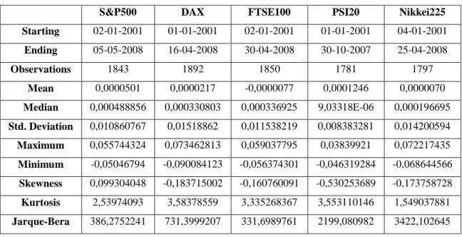
The descriptive statistics of the returns of these indexes, based on the in-sample data, are presented in Table 3:
Table 3. Summary Statistics of Returns (In-sample)
S&P500 DAX FTSE100 PSI20 Nikkei225
Starting 02-01-2001 01-01-2001 02-01-2001 01-01-2001 04-01-2001 Ending 05-05-2008 16-04-2008 30-04-2008 30-10-2007 25-04-2008 Observations 1843 1892 1850 1781 1797 Mean 0,0000501 0,0000217 -0,0000077 0,0001246 0,0000070 Median 0,000488856 0,000330803 0,000336925 9,03318E-06 0,000196695 Std. Deviation 0,010860767 0,01518862 0,011538219 0,008383281 0,014200594 Maximum 0,055744324 0,073462813 0,059037795 0,03839921 0,072217435 Minimum -0,05046794 -0,090084123 -0,056374301 -0,046319284 -0,068644566 Skewness 0,099304048 -0,183715002 -0,160760091 -0,530253689 -0,173758728 Kurtosis 2,53974093 3,58378559 3,335268367 3,553110146 1,549037881 Jarque-Bera 386,2752241 731,3999207 331,6989761 2199,080982 3422,102645
As we can see, according to the results presented in the in-sample analysis, contrary to the ones presented in the whole sample, we can see that most of the indexes have a positive mean. One of the reasons for this situation is the fact that in these sample are not considered
12
the last 3/4 years (mid 2008 to 2011), when the world crisis had and has an extreme impact on the assets’ returns, thus suffering a decrease, and consequently contributing for the negative mean, if we consider the whole sample.
However, most of the indexes continue to have an asymmetry, with a heavier and longer left tail, except for S&P 500, which has a longer right tail, but the value seems to be significant. The kurtosis implies that all of them are leptokurtic, and the Jarque-Bera test results confirm the rejection of the normality assumption, the same conclusions as if we consider the whole sample.
3.2.2. Estimation Results
According to Bollerslev, Chou and Kroner (1992), and more recently, Hansen and Lunde (2005), the use of model is satisfactory when estimating the volatility of financial assets. Since most of the empirical papers deal with this specification, Medeiros and Veiga (2009) focused their attention on a first-order FCGARCH specification. Thus, when estimating the FCGARCH model, and in order to compare it with EGARCH and GJR, we are going to use this specification.
Moreover, when estimating the volatility using the FCGARCH model, due to the complexity of the estimation of the regimes in Matlab, and since in Medeiros and Veiga (2009) paper most of their estimated results were based on 3 regimes, we are going to use that assumption in our estimation, that is, H=2.
According to Franses and Van Dijk (2000), as well as Fan and Yao (2003), since we don’t know the “true” distribution of the innovations/news, the use of QML can provide a practical way to estimate non-normal GARCH parameters, being much more simple its estimation. So, in order to compare the in-sample results, we are going to use the quasi maximum log-likelihood (QML) on the three models, so we can make a more realistic analysis and comparison.
The use of this estimator assumes that the innovations follow a normal distribution, although it can also be used for non-normal distributions, such as Student t (1925), for example. Medeiros and Veiga (2009) used the QML in their paper, so we are going to do the
13
same. Since the FCGARCH model properties were developed for the normal distribution, we will also assume in this thesis that the innovations follow a Gaussian (Normal) distribution.
It is also to be acknowledged that, although we have seen that the observations for this thesis seem to follow a non-normal distribution, as seen in the results for the Jarque-Bera test, the use of FCGARCH, according to Medeiros and Veiga (2009: 117), has the main advantage of “generating series with high kurtosis”, so the assumption for the normality of the innovations is plausible for this thesis.
The codes which were used for the estimation of the three models were made on Matlab program, and are present in annexes 1.2. It is to note the complexity of the FCGARCH model and consequently of its incorporation in Matlab, due to the number of parameters and regimes incorporated in the model. However, in this thesis we have reached a point where all the conditions are satisfied, the parameters seem reasonable, if compared to the ones predicted by Medeiros and Veiga (2009), and it was created a prediction code of FCGARCH, all of them working, with no errors whatsoever, thus contributing for a better interpretation and conclusion of the results presented in this thesis.
It is also to note, since I created the codes for the FCGARCH model, in order to make a plausible comparison between the models in study, I thought it would be better if I created not only the estimation codes for the FCGARCH, but also for EGARCH and GJR models. With the use of these codes, based on the in-sample observations, we reach the following results, presented on tables 4, 5 and 6:
14 Table 4. Estimation Results
Parameters S&P 500 DAX 30
EGARCH GJR FCGARCH EGARCH GJR FCGARCH
-0,2618 1,5508E-06 - -0,2792 2,85E-06 - 0,0851 0 1,0000E-06 0,1192 0 3,1822E-06 0,9792 0,9149 1,2028 0,9786 0,901 1,3006 - - 0,0737 - - 0,0701 - - 2,6376E-06 - - -7,3908E-07 - - -0,3242 - - -0,4881 -0,1222 1,1377 -0,0737 -0,1246 0,1671 0,0381 - - -0,72 - - -0,72 - - 2,52 - - 2,52 - - -2,6376E-06 - - 3,0621E-05 - - -0,3326 - - -0,4882 - - 0,0713 - - -0,0759 - - 1,56 - - 1,56 - - 2,85 - - 2,85 Quasi-Log-Likelihood
6.0149e+03 6.0066e+003 6.0188e+003 5.6624e+03 5.6616e+03 5.6558e+03
Akaike Information
Criterion
-1,2030E+08 -1,2013E+08 -1,2038E+08 -1,1325E+08 -1,1323E+08 -1,1312E+08
Schwarz Bayesian Criterion
15 Table 5. Estimation Results
Parameters FTSE 100 EGARCH GJR FCGARCH -0,2821 1,83E-06 - 0,1098 0 1,0000E-08 0,9795 0,8881 1,2968 - - 0,0565 - - 2,4500E-06 - - -0,4717 -0,151 0,1839 0,0569 - - -0,72 - - 2,52 - - -2,4500E-06 - - -0,4636 - - -0,0562 - - 1,56 - - 2,85
Quasi-Log-Likelihood 6.0696e+03 6.0627e+003 6.0785e+003
Akaike Information
Criterion -1,2139E+08 -1,2125E+08 -1,2157E+08
Schwarz Bayesian
16 Table 6. Estimation Results
Parameters
Nikkei 225 PSI 20
EGARCH GJR FCGARCH EGARCH GJR FCGARCH
-0,3609 2,98E-06 - -1,5266 4,49E-06 - 0,1704 0,0356 9.0685E-07 0,2139 0,048 4,7407E-05 0,9736 0,9041 1,1994 0,8584 0,8102 0,5225 - - 0,0640 - - 0,7731 - - -8.9685E-07 - - -3,9627E-05 - - -0,2884 - - 0,0324 -0,0785 0,0941 -0,0640 -0,1589 0,1625 -0,7731 - - -0,72 - - -0,72 - - 2,52 - - 2,52 - - 4.1674E-05 - - 1,4257E-05 - - -0,6589 - - -0,5549 - - 0,1162 - - 0,2080 - - 1,56 - - 1,56 - - 2,85 - - 2,85
Quasi-Log-Likelihood 5.2486e+003 5.2465e+003 5.2634e+003 6.1476e+03 6.1638e+003 6.1319e+003
Akaike Information
Criterion
-1,0497E+08 -1,0493E+08 -1,0527E+08 -1,2295E+08 -1,2328E+08 -1,2264E+08
Schwarz Bayesian Criterion
17
As we can see, the in-sample estimation results confirm the high sensitivity of the market according to the “bad news”, since the sign of the parameter is negative in the EGARCH and positive in the GJR. The same happens in FCGARCH model, since each regime is related to certain kinds of innovations, as explained before and seen in the tables.
We can also see, in the case of the S&P500, DAX30 and FTSE indexes, we have an which is exactly 0 in the GJR model, according to the codes created for this thesis. Since the parameter is combined with the dummy related to bad news, we can conclude that future positive news have no impact at all in the future volatilities, thus focusing mainly on the leverage effect explained before.
Another point worth of mentioning is the fact that, in the FCGARCH model, the and parameters are exactly the same in all the indexes estimated. However, these parameters are only related to the transition between regimes, and since the conditions are satisfied, the logistic function is considered a smooth transition function in the FCGARCH model linking the regimes included in the model. So, our main focus will be on the GARCH parameters of the FCGARCH model, that is, the , and .
As we can also see, the Quasi-Maximum-Log-Likelihood, which its results show how well the data is incorporated in the models, testing how the data used for the estimation is more likely to fit in a certain model than in another, shows positive values for all the models studied in this thesis. Since Matlab cannot maximize, thus can only minimize, the codes present in annex 1.2.1. show a negative function for the QML, thus showing the most negative possible value. So, the sign of the output must be changed, which means that the results shown in Matlab should be changed back to positive values, as seen in tables 4, 5 and 6.
According to the Quasi-Maximum-Log-Likelihood, we see that the FCGARCH model has the highest values, mainly on S&P 500, FTSE 100 and Nikkei 225 indexes, being GJR the best model in PSI 20 and DAX 30.
One thing that it is to note, is the fact that, although the FCGARCH has the main advantage of modeling more than two limiting regimes, and has a higher QML in some of the indexes studied, this model’s QML result is very close to the ones from EGARCH and GJR. Since the model deals with a high number of parameters, contrary to EGARCH and GJR, the
18
FCGARCH may fail in some goodness-of-fit measures, such as Akaike Information Criterion (1978):
, (19)
as well as Schwarz Bayesian Criterion (1978):
, (20)
being the number of parameters in the model, the number of observations used for the estimation, and the Log-Likelihood function, which, in this case, will be the Quasi-Maximum-Log-Likellihood.
The main characteristic of these criterions is the fact that they are based mainly on the number of parameters estimated: the less parameters the model uses, the more likely it is the best model. However, as we can see, the results confirm the QML conclusions, showing that the FCGARCH model seems to be the best one in S&P 500, FTSE 100 and Nikkei 225, since it has the lowest values from the three models presented. Regarding DAX 30 and PSI 20, the results favour EGARCH and GJR, respectively.
In conclusion, by looking at the parameters’ estimation results, and at the QML, we see that FCGARCH and GJR models seem to be the most prone to generate and predict the future data.
3.3.Out-of-sample Analysis - Results
In order to check which of the models studied in this paper predicts best the volatilities in-sample, we use the quasi-log-likelihood maximum value. However, for the out-of-sample, there is also a volatility forecast comparison test, proposed by Harvey and Newbold (2000), for multiple surrounding forecasts.
Assuming that are the competing forecasts, made one-step ahead with non-autocorrelated errors, of the actual quantity , the test can be written by the following formula:
19
It is to note that , with , with , and is the error of the combined forecast. Thus, we can write the regression in its matrix general form, being the following:
and (22)
Where , and . The F test used for this case is an F test of the joint significance of the parameters of , being the null hypothesis the fact that encompasses , that is:
The codes which were used for the test of these three models were made on E-views program, by my supervisor, Professor José Dias Curto, and are present in annex 1.2.3. What I have made is comparing one model according to the 2 competing ones, and test their joint significance, applying the out-of-sample observations, according to the hypothesis shown before, thus testing the predictive capability of the models in study.
In order to use the Harvey-Newbold test I have created a volatility prediction code for the FCGARCH model in Matlab, present in annex 1.2.2.1. The predictions for the variances of the other two models were made by hand, using the Microsoft Excel.
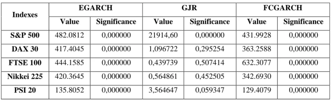
Table 6 shows the results for using the Harvey-Newbold test for the forecasts of the 5 indexes, according to the models studied in this paper.
Table 6. Harvey-Newbold Test Indexes
EGARCH GJR FCGARCH
Value Significance Value Significance Value Significance
S&P 500 482.0812 0,000000 21914,60 0,000000 431.9928 0,000000
DAX 30 417.4045 0,000000 1,096722 0,295254 363.2588 0,000000
FTSE 100 444.1585 0,000000 0,439739 0,507414 632.3077 0,000000
Nikkei 225 420.3645 0,000000 0,564861 0,452505 342.6930 0,000000
PSI 20 135.8052 0,000000 3,564647 0,059347 129.4079 0,000000
The results seem to favour the GJR model in 4 out of 5 indexes, where we fail to reject the null that the GJR forecasts can’t be improved by combination with the other two models, except for S&P 500, where the null is rejected (for a 5% significance level), which means that
20
the FCGARCH and/or EGARCH predictions, with the ones from GJR, would lead to an improvement of the S&P 500 index forecast performance. However, since the FCGARCH presents a much lower value, although the test is not statistically significant, we can conclude that the FCGARCH seems better to encompass EGARCH and GJR in this index, thus seeming to be a better model than EGARCH and GJR.
21
4. Conclusions
Nowadays, due to the complexity and constant fastness of how the information is passed throughout the world, it is very difficult not only to predict the price of a certain asset, but also to forecast its volatility. Therefore, there is a need to create a model which can be used in order to make the most rightful decision.
Several regularities of these assets have been discovered, and consequently, several models have been determined, with the most popular ones being GARCH models, namely EGARCH, GJR and FCGARCH. The main purpose of this thesis was to discover which one of these models seems better to predict the financial markets’ volatility.
The empirical analysis is based on the daily returns of 5 most important international stock market indexes, such as S&P 500 (USA), FTSE 100 (UK), DAX 30 (Germany), PSI 20 (Portugal), and Nikkei 225 (Japan). These returns, from January 2001 to December 2011, were divided in two main periods, being the first 2/3 used for the estimation of the parameters, and the final 1/3 for the forecast period.
According to the estimation in-sample results based on the codes created in Matlab for all three models, based on the Quasi-Maximum-Likelihood, the FCGARCH model seem to be the best in S&P 500, FTSE 100 and Nikkei 225 indexes, fitting the dynamics of the returns of the indexes in study.
If we consider other goodness-of-fit measures, such as Akaike and Schwarz criterions, the results confirm the QML conclusions, showing that the FCGARCH model, although it has a significant number of parameters, seems to be the best one in the same indexes, since it has the lowest values from the three models presented. These criterions also seem to favour the GJR model.
The out-of-sample results, based on the Harvey-Newbold encompassing test, based on the codes created in E-views, show that the best model to predict the volatility forecasts for the majority of the indexes under study, seems to be not FCGARCH, but the GJR model.
Some of the limitations and future research that should be considered in this thesis are the following ones:
The fact that, first, we assume that the observation’s returns follow a normal distribution, when in fact, the descriptive statistics show the opposite (a non-normal
22
distribution). Thus, it could be useful to use other distributions than the Gaussian one in this study, such as Student t (1925), for example.
According to Andersen and Bollerslev (1998), the use the daily squared returns as a proxy of daily volatility can be considered a noisy estimator, which may lead us to use an alternative proxy for the daily volatility, such as the intraday realized volatility, for example.
For this thesis, the in-sample observations do not include the financial crisis period started in 2008. It could be a plus if we could separate the in-sample data and the out-of-sample data in a more convenient way, thus considering the extreme variances of the returns of the indexes in these last years.
In this thesis we used the PSI20 index, a Portuguese one which was not considered in the paper by Medeiros and Veiga (2009). It could be considered for future analysis other indexes than the ones studied, not also in their paper but also in this thesis. Lastly, it is to note that the variance estimated coefficients for the three models in this
thesis do not have their significance measure for the errors, thus not knowing if they are statistically significant and thus plausible for study. However, the main objective of this thesis was to compare the models, obtaining the maximum value for the QML, thus knowing which of the models seems to be the best one to describe the volatility. For future research, it should be considered a measure for the significance of the estimated coefficients.
This thesis and its empirical result tends to be useful for those who want to get deeper in the FCGARCH model, and study its advantages, disadvantages, parameters and results, thus being closer to find the best model, regarding the forecast of volatility in financial markets, mainly during periods of high volatility.
23
References
Akaike, H. 1978. Time series analysis and control through parametric models. Applied time
series analysis, D. F. Findley (ed.). New York: Academic Press
Andersen, T.G. & Bollerslev, T. (1998). Answering the skeptics: yes, standard volatility models do provide accurate forecasts. International Economic Review, 39: 885-905.
Bachelier, L. 1990. Théorie de la Spéculation. Annales Specifiques de l’É.N.S. 3e série, tome 17: 21-86
Bollerslev, T. 1986. Generalized autoregressive conditional heteroskedasticity, Journal of
Econometrics. 21: 307-327
Bollerslev, T., Chou, R., & Kroner, K. 1992. ARCH modeling in finance. Journal of
Econometrics, 52: 5-59
Black, F. 1976. Studies in stock price volatility changes. ASA Proceedings, Business and
Economic Statistics: 177-181
Christie, A. A. 1982. The stochastic behavior of common stock variances: value, leverage and interest rate effects. Journal of Financial Economics, 10: 407-432
Costa, R. 2010. Risk Neutral Option Pricing under some special GARCH models. Ph.D. Dissertation, Pontifícia Universidade Católica do Rio de Janeiro
Engle, R. F. 1982. Autoregressive conditional heteroskedasticity with estimates of the variance of United Kingdom inflation. Econometrica, 50: 987-1008
Fan, J., & Yao, Q. 2003. Nonlinear Time Series: Nonparametric and Parametric Models. Springer-Verlag, New York
Fisher, R. A. 1925. Applications of "Student's" distribution. Metron, 5: 90–104
Franses, P. H.; Van Dijk, D. 2000. Non-linear Time Series Models in Empirical Finance. Cambridge University Press, Cambridge
Glosten L., Jagannathan, R., & Runkle, R. 1993. On the relationship between the expected value and the volatility of the nominal excess returns on stocks. Journal of Finance, 48: 1779-1801
Hagerud, G. E. 1997. A new non-linear GARCH Model. Ph.D. Dissertation, Stockholm School of Economics
Hansen, P., & Lunde, A. 2005. A forecast comparison of volatility models: does anything beat a GARCH(1,1)?. Journal of Applied Econometrics, 20: 873-889
Harvey, D., & Newbold, P. 2000, Tests for multiple forecast encompassing. Journal of
Applied Econometrics, 15: 471-482
Hillebrand, E., & Medeiros M.C. 2008, Estimating and forecasting GARCH models in the presence of structural breaks and regime switches. Frontiers of Economics and Globalization, vol. 3: 303-327
24
Jarque, C., M. & Bera, A. K., 1987. A test for normality of observations and regression residuals. International Statistical Review, 2: 163-172
Jeantheau, T. 1998. Strong consistency of estimates for multivariate ARCH models,
Econometric Theory, 14: 70-86
Lee, S. -W. & Hansen, B. E. 1994. Asymptotic theory for the GARCH(1,1) quasi-maximum likelihood estimation. Econometric Theory, 10: 29-52
Ling, S., & McAleer, M. 2003. Asymptotic theory for a vector ARMA-GARCH model,
Econometric Theory, 19: 280-310
Majmudar, U., & Banerjee, A. 2004. VIX Forecasting. The 40th Annual Conference of the Indian Econometrics Society
Mandelbrot, B. 1963. The variation of certain speculative prices. Journal of Business, 36: 394-419
Medeiros, M. C, & Veiga, A. L. 2009. Modeling multiple regimes in financial volatility with a flexible coefficient GARCH(1,1) model, Econometric Theory, 25: 117-161
Nelson, D.B. 1991. Conditional Heteroskedasticity in asset returns: A new approach.
Econometrica, 59: 347-370
Salgado, J. 2011. What best predicts realized and implied volatility: GARCH, GJR or FCGARCH?. Master in Finance, ISCTE.
Schwarz, G. 1978. Estimating the dimension of a model, Annals of statistics, 6: 461-64 Schwert, G. W. 1989. Business cycles, financial crisis, and stock volatility.
25
Jan 2001 Jan 2003 Jan 2005 Jan 2007 Jan 2009 Jan 2011 Dec 2011 2000 3000 4000 5000 6000 7000 8000 9000
DAX 30 Daily Closing Prices
Jan 2001 Jan 2003 Jan 2005 Jan 2007 Jan 2009 Jan 2011 Dec 2011 3000 3500 4000 4500 5000 5500 6000 6500 7000
FTSE100 Daily Closing Prices
Jan 2001 Jan 2003 Jan 2005 Jan 2007 Jan 2009 Jan 2011Dec 2011 5000 6000 7000 8000 9000 10000 11000 12000 13000 14000
PSI20 Daily Closing Prices
Jan 2001 Jan 2003 Jan 2005 Jan 2007 Jan 2009 Jan 2011 Dec 2011 600 700 800 900 1000 1100 1200 1300 1400 1500 1600
S&P500 Daily Closing Prices
Jan 2001 Jan 2003 Jan 2005 Jan 2007 Jan 2009 Jan 2011Dec 2011 -0.1 -0.05 0 0.05 0.1 0.15
DAX 30 Daily Returns
Jan 2001 Jan 2003 Jan 2005 Jan 2007 Jan 2009 Jan 2011 Dec 2011 -0.1 -0.08 -0.06 -0.04 -0.02 0 0.02 0.04 0.06 0.08 0.1
FTSE100 Daily Returns
Jan 2001 Jan 2003 Jan 2005 Jan 2007 Jan 2009 Jan 2011 Dec 2011 -0.2 -0.15 -0.1 -0.05 0 0.05 0.1 0.15
PSI20 Daily Returns
0 Jan 2003 Jan 2005 Jan 2007 Jan 2009 Jan 2011 Dec 2011 -0.1 -0.05 0 0.05 0.1 0.15
S&P500 Daily Returns
Jan 20010.6 Jan 2003 Jan 2005 Jan 2007 Jan 2009 Jan 2011 Dec 2011 0.8 1 1.2 1.4 1.6 1.8 2x 10
4 Nikkei225 Daily Closing Prices
Jan 2001 Jan 2003 Jan 2005 Jan 2007 Jan 2009 Jan 2011 Dec 2011 -0.2 -0.15 -0.1 -0.05 0 0.05 0.1 0.15
NIKKEI225 Daily Returns
Annexes
26 1.2.Matlab Codes 1.2.1. Estimation of Parameters 1.2.1.1.EGARCH clear all; close all; clear global; clc; global x; x=xlsread('C:\...\*.xlsx'); T=size(x,1); h(1)=x(1)^2; constant = 0.0005; alpha = 0.15; beta = 0.8; gama = -0.04; x0=[constant,alpha,beta,gama];
options = optimset('Algorithm','sqp','display', 'iter','TolX', 1e-14,
'TolCon',1e-14, 'TolFun', 1e-14, 'MaxFunEvals', 2000);
[parameters, fval,exitflag,output] =
fmincon('objfunegarch',x0,[],[],[],[],[],[],'confunegarch',options,x)
function [cons, ceq] = confunegarch(parameters,x)
T=size(x,1);
constant = parameters(1); alpha = parameters(2); beta = parameters(3); gama = parameters(4);
% Nonlinear inequality constraints; note: make (...)<0
cons = [gama;
abs(beta)-0.9999999999999];
% Nonlinear equality constraints
ceq = [] ;
function likeli = objfunegarch(parameters,x)
constant = parameters(1); alpha = parameters(2); beta = parameters(3); gama = parameters(4); T=size(x,1); h(1)=(x(1))^2; for t=2:T; h(t,1)=exp(constant+alpha*(abs(x(t-1,1))/((h(t-1))^(1/2)))+gama*(x(t-1,1)/((h(t-1))^(1/2)))+beta*log((h(t-1))^2)); end
27
likeli=T*((1/T)*sum((1/2)*log(2*pi)+(1/2)*log(h)+(x.^2)./(2*h))); %note:
used – because matlab can’t maximize. There are points after x because x is a vector. end 1.2.1.2.GJR clear all; close all; clear global; clc; global x; x=xlsread('C:\...\*.xlsx'); T=size(x,1); h(1)=x(1)^2; constant = 0.0005; beta = 0.8; lambda = 0.15; gama = 0.04; x0=[constant,beta,lambda,gama];
options = optimset('Algorithm','sqp','display', 'iter','TolX', 1e-14,
'TolCon',1e-14, 'TolFun', 1e-14, 'MaxFunEvals', 2000);
[parameters, fval,exitflag,output] =
fmincon('objfun2012gjr',x0,[],[],[],[],[],[],'confun2012gjr',options,x)
function [cons, ceq] = confun2012gjr(parameters,x)
T=size(x,1); constant = parameters(1); beta = parameters(2); lambda = parameters(3); gama = parameters(4);
% Nonlinear inequality constraints; note: make (...)<0
cons = [-constant; -beta; -lambda; -lambda-gama;
beta+lambda+(1/2)*gama-1];
% Nonlinear equality constraints
ceq = [] ;
function likeli = objfun2012gjr(parameters,x)
constant = parameters(1); beta = parameters(2); lambda = parameters(3); gama = parameters(4);
28 T=size(x,1); h(1)=(x(1))^2; dummy=0; for t=2:T; if x(t-1)<0; dummy=1; else dummy=0; end h(t,1)=constant+(lambda+gama*dummy)*x(t-1)^2+beta*h(t-1); end likeli=T*((1/T)*sum((1/2)*log(2*pi)+(1/2)*log(h)+(x.^2)./(2*h))); %note:
used – because matlab can’t maximize. There are points after x because x is a vector. end 1.2.1.3.FCGARCH clear all; close all; clear global; clc; global x; x=xlsread('C:\...\*.txt'); H=2; T=size(x,1); h=ones(T,1); h(1)=x(1)^2; alphas= [2.22*(10^-16), 2.55*(10^-5), 3.73*(10^-4) ]; betas=[1.21, -0.32, -0.25]; lambdas=[0.06,-0.01,-0.04]; c=[-0.72,1.56]; gama=[2.52,2.85]; x0=[alphas,betas,lambdas,c,gama];
options = optimset('Algorithm','sqp','display', 'iter','TolX', 1e-14,
'TolCon',1e-14, 'TolFun', 1e-14, 'MaxFunEvals', 1500);
[parameters, fval,exitflag,output] =
fmincon('objfun2012',x0,[],[],[],[],[],[],'confun2012',options,x)
function [cons, ceq] = confun2012(parameters,x)
T=size(x,1); alphas = parameters(1:3); betas = parameters(4:6); lambdas = parameters(7:9); c = parameters(10:11); gama = parameters(12:13);
sum_alphas= cumsum(alphas); %cum sum A=[1,2,3]; cumsum(A) = [1,3,6]
sum_betas= cumsum(betas); sum_lambdas= cumsum(lambdas);
29
% Nonlinear inequality constraints; note: make (...)<0
cons = [-c(2)+c(1)+(10^-8); %assumption 3 r1; +10^-18 because it’s
strictly positive
-c(1)-realmax; %assumption 3 r1; realmax = best MATLAB
approximation to infinity -c(2)-realmax; %assumption 3 r1 -gama(1)+10^-18; %assumption 3 r2 -gama(2)+10^-18; %assumption 3 r2 -sum_alphas(1)+10^-8; -sum_alphas(2)+10^-8; %assumption 5 r1; -sum_alphas(3)+10^-8; -(1./(1+exp(-gama(1)*(x-c(1)))))+(1./(1+exp(-gama(2)*(x-c(2)))));
%assumption 4; There are points after 1 because 1 is a vector.
-sum_betas(1); %assumption 5 r2 -sum_betas(2); -sum_betas(3); -sum_lambdas(1); %assumption 5 r3 -sum_lambdas(2); -sum_lambdas(3); (1./(1+exp(-gama(1)*(x-c(1)))))+(1./(1+exp(gama(1)*(x-c(1)))))-1; % assumption 9 (1./(1+exp(-gama(2)*(x-c(2)))))+(1./(1+exp(gama(2)*(x-c(2)))))-1; (1/2)*(2*betas(1)+betas(2)+betas(3)+2*lambdas(1)+lambdas(2)+lambdas(3))-1+10^-18;%assumption 7 betas(1)^2+betas(1)*(betas(2)+betas(3))+(((betas(2)+betas(3))^2)/2)+(sum(x. ^4)/T)*(lambdas(1)+lambdas(1)*(lambdas(2)+lambdas(3))+((lambdas(2)+lambdas( 3))^2)/2)+2*lambdas(1)*betas(1)+betas(1)*(lambdas(2)+lambdas(3))+lambdas(1) *(betas(2)+betas(3))+(lambdas(2)+lambdas(3))*(betas(2)+betas(3))-1+10^-18 %assumption 10 ];
% Nonlinear equality constraints
ceq = [] ;
function likeli = objfun2012(parameters,x)
alphas = parameters(1:3); betas = parameters(4:6); lambdas = parameters(7:9); c = parameters(10:11); gama = parameters(12:13); H=2; T=size(x,1); h(1)=(x(1))^2; for t=2:T; regi(1)=alphas(1)+betas(1)*h(t-1)+lambdas(1)*x(t-1)^2; for j=1:H; if (1/(1+exp(-gama(j)*(x(t-1)-c(j))))) <0 disp('AFFLog') end regi(j+1)=(alphas(j+1)+betas(j+1)*h(t-1)+lambdas(j+1)*x(t-1)^2)*(1/(1+exp(-gama(j)*((x(t-1)/(h(t-1))^(1/2))-c(j))))); regac=sum(regi); end
30 h(t,1)=regac; if min(h)<0 disp('AFF') h pause end end likeli=T*((1/T)*sum((1/2)*log(2*pi)+(1/2)*log(h)+(x.^2)./(2*h)));
%note: used – because matlab can’t maximize. There are points after x because x is a vector. end 1.2.2. Forecasting Returns 1.2.2.1.FCGARCH clear all clc H=2; T=899; k=1000; %number of simulations p=13863.47; %closing price at t-1 tic
%using estimated results of the parameters (for each index)
alpha=[1.5152*10^-05,-8.1461*10^-06,-6.9958*10^-06]; beta=[1.1994,-0.2884,-0.6589];
lambda=[0.0640,-0.0640,0.1122]; gama=[-0.72,1.56];
c=[2.52,2.85];
sigma=0.3; %initial value for sigma
sigma2=sigma^2; diasnoano=360;
h(1:k,1)=((sigma2)/diasnoano);
Nor=randn(k,T); % creates random numbers, which will be the noises. It will
be created a number of vectors throughout the simulations for i=1:k; y(i,1)=h(i,1)^(1/2)*Nor(i,1); for t=2:T; regi(1)=alpha(1)+beta(1)*h(i,t-1)+lambda(1)*(h(i,t-1)^(1/2)*Nor(i,t-1))^2; for j=1:H; regi(j+1)=(alpha(j+1)+beta(j+1)*h(i,t-1)+lambda(j+1)*(h(i,t-1)^(1/2)*Nor(i,t-1))^2)*(1/(1+exp(-gama(j)*(y(i,t-1)-c(j))))); regac=sum(regi); end h(i,t)=regac; if h(i,t)<0; h(i,t)=0.0000001; end
31 y(i,t)=h(i,t)^(1/2)*Nor(i,t);
end
end
retornoac=sum(y,2); sum of y throughout the lines (,2)
ST=p*(exp(retornoac)) toc 1.3. E-views Codes 1.3.1. Harvey-Newbold Test series e1t=rt2-sigfcgarch vector(1000) yt stomna(e1t, yt) series e2t=rt2-sigegarch series e3t=rt2-siggjr series de12t=e1t-e2t series de13t=e1t-e3t equation eq3
eq3.ls e1t de12t de13t show eq3.output !obs=@obssmpl !s2=@se^2 !K=@ncoef eq3.makeresids res1 vector(1000) resf1 stomna(res1, resf1) vector(!K) LAMB for !i=1 to !K LAMB(!i)=@coefs(!i) next matrix(1000,2) X
group HNg1 de12t de13t stomna(HNg1, X) matrix(1000,2) HatM matrix(1000,2) HatQ matrix(1000,2) HatD HatM=(!obs^-1)*@transpose(X)*X HatQ=!s2*HatM HatD=@inverse(HatM)*HatQ*@inverse(HatM) 'F standard test matrix(1,1) F11 F11=@transpose(lamb)*@inverse(HatD)*lamb scalar F=!obs*(!K-1)^(-1)*@trace(F11) !ProbF=1-@cfdist(F,!K-1,!obs-!K+1) 'Computing F1 !q=0 !cm=@columns(HatM) !rm=@rows(HatM) matrix(!cm, !rm) HatQ1 for !i=1 to !cm for !j=1 to !rm for !l=1 to !obs !q=!q+X(!l, !i)*X(!l,!j)*resf1(!l)^2
32 next HatQ1(!i,!j)=!q*!obs^(-1) !q=0 next next matrix(!rm, !cm) HatD1 HatD1=@inverse(HatM)*HatQ1*@inverse(HatM) matrix(1,1) F12 F12=@transpose(lamb)*@inverse(HatD1)*lamb scalar F1=!obs*(!K-1)^(-1)*@trace(F12) !ProbF1=1-@cfdist(F1,!K-1,!obs-!K+1) 'Computing F1 !q=0 !cm=@columns(HatM) !rm=@rows(HatM) matrix(!cm, !rm) HatQ2 for !i=1 to !cm for !j=1 to !rm for !l=1 to !obs !q=!q+X(!l, !i)*X(!l,!j)*yt(!l)^2 next HatQ2(!i,!j)=!q*!obs^(-1) !q=0 next next matrix(!rm, !cm) HatD2 HatD2=@inverse(HatM)*HatQ2*@inverse(HatM) matrix(1,1) F13 F13=@transpose(lamb)*@inverse(HatD2)*lamb scalar F2=!obs*(!K-1)^(-1)*@trace(F13) !ProbF2=1-@cfdist(F2,!K-1,!obs-!K+1) 'COMPUTING MS* scalar MS=(!obs-(!K-1)*F2)^(-1)*(!obs-!K+1)*F2 !ProbMS=1-@cfdist(MS,!K-1,!obs-!K+1) series dmsv1=(sigfcgarch-rt2)^2 'MAE MSV-EGARCH series dmsv2 dmsv2=@abs(sigfcgarch-rt2) show resulta