Controle preditivo multi-modelos baseado em LMIs para sistemas estáveis e instáveis...

(1)

BRUNO DIDIER OLIVIER CAPRON

LMI-based Model Predictive Control of uncertain stable and unstable systems based on a realigned state space representation

(2)

Tese apresentada à Escola Politécnica da Universidade de São Paulo para obtenção do título de Doutor em Ciências

(3)

Este exemplar foi revisado e corrigido em relação à versão original, sob responsabilidade única do autor e com a anuência de seu orientador. São Paulo, de agosto de 2014.

Assinatura do autor ____________________________

Assinatura do orientador _______________________

Catalogação-na-publicação

Capron, Bruno Didier Olivier

LMI-based Model Predictive Control of uncertain stable and unstable systems based on a realigned state space representa-tion / B.D.O. Capron. – versão corr. -- São Paulo, 2014.

190 p.

Tese (Doutorado) - Escola Politécnica da Universidade de São Paulo. Departamento de Engenharia Química.

(4)

Tese apresentada à Escola Politécnica da Universidade de São Paulo para obtenção do título de Doutor em Ciências

Área de Concentração: Engenharia Química

Orientador: Prof. Dr. Darci Odloak

(5)

ACKNOWLEDGEMENTS (In portuguese)

Ao professor Darci Odloak por ter me dado a oportunidade de trabalhar neste projeto, pela disponibilidade, pela atenção e pela competência na orientação desta tese.

Aos professores Claudio Garcia, Luiz Cláudio e Galo Leroux, aos doutores Zanin e Lincoln Moro pela dedicação na leitura da tese e pelas sugestões de melhoria dadas tanto durante o exame de qualificação quanto durante a defesa.

Aos companheiros do Laboratório de Simulação e de Controle de Processos pela boa companhia.

À minha família pelo suporte e pela compreensão.

À minha namorada pelo carinho e pelo apoio.

(6)

RESUMO

(7)

(8)

ABSTRACT

(9)

(10)

LIST OF FIGURES

Figure 2-1 : Zone control and input target strategy structure ... 8 Figure 3-1: Schematic representation of the PP splitter ... 28 Figure 3-2: Outputs with the IHMPC-OPOM (───), outputs with the IHMPC-RM

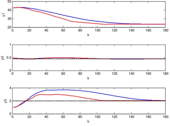
(───) and output zone limits (─ ─ ─). First part of simulation ... 30

Figure 3-3: Inputs with the IHMPC-OPOM (───), inputs with the IHMPC-RM (───)

and input targets (─ ─ ─). First part of simulation ... 31

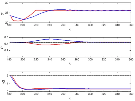
Figure 3-4: Outputs with the IHMPC-OPOM (───), outputs with the IHMPC-RM

(───) and output zone limits (─ ─ ─). Second part of simulation ... 33

Figure 3-5: Inputs with the IHMPC-OPOM (───), inputs with the IHMPC-RM (── ─) and input targets (─ ─ ─). Second part of simulation ... 34

Figure 4-1: Schematic representation of a FCC unit ... 58 Figure 4-2: Outputs with the LMI-based MPC (───) and the NLP-based MPC (───),

and bounds (− − −). Multi-plant uncertainty ... 62 Figure 4-3: Inputs with the LMI-based MPC (────) and the NLP-based MPC

(────_{) and targets (}······_{). Multi-plant uncertainty ... 63}

Figure 4-4: Upper bound to the cost function of the true plant with the LMI-based MPC. Multi-plant uncertainty ... 64 Figure 4-5: Outputs with the LMI-based MPC (────), bounds (− − −) and setpoints

(······). Switching nominal model ... 67

Figure 4-6: Inputs with the LMI-based MPC (────) and targets (······). Switching

nominal model ... 68 Figure 4-7: Upper bound to the cost function of the true plant with the LMI-based MPC. Switching nominal model ... 68 Figure 4-8: Outputs with the LMI-based MPC (────) and bounds (− − ). Polytopic

uncertainty. ... 70 Figure 4-9: Inputs with the LMI-based MPC. Polytopic uncertainty. ... 71 Figure 4-10: Upper bound to the cost function of the true plant with the LMI-based MPC. Polytopic uncertainty. ... 72 Figure 4-11: Schematic representation of the C3/C4 splitter ... 73 Figure 4-12: Operating window of the C3/C4 splitter obtained with a rigorous process simulator ... 75 Figure 4-13 : Outputs with the LMI-based MPC (───) and with the NLP-based MPC

(───). Calculated setpoints with the LMI-based MPC (──) and with the NLP-based

MPC (──) and control zones (− − −). ... 78

Figure 4-14: Manipulated inputs with the LMI-based MPC (───) and with the

NLP-based MPC (───) and targets(− − −). ... 79

Figure 4-15: Measured disturbances. Second simulation. ... 80 Figure 4-16: Outputs with the LMI-based MPC (───) and with the NLP-based MPC

MPC (──) and bounds(− − −). ... 82

(11)

Figure 4-18: Measured disturbances. Third simulation. ... 84 Figure 4-19: Outputs with the LMI-based MPC (───) and with the NLP-based MPC

MPC (──) and bounds(− − −). ... 86

NLP-based MPC (───) and targets (− − −). ... 87

Figure 5-1: Schematic representation of the combined LQR-MPC approach ... 93 Figure 5-2: Input limits (───), input targets (───), input with the LQR-MPC (───)

and inputs with the conventional MPC (───) ... 114

Figure 5-3: Outputs with the LQR-MPC (───), output setpoints with the LQR-MPC

(───), outputs with the conventional MPC (───) and output zones (───) ... 116

Figure 5-4: Real plant cost Vk with the LQR-MPC ... 118

Figure 5-5: Input limits (───), input targets (───), input with the LQR-MPC (───)

and inputs with the conventional MPC (───) ... 120

Figure 5-6: Outputs with the LQR-MPC (───), output setpoints with the LQR-MPC

(───), outputs with the conventional MPC (───) and output zones (───) ... 122

Figure 5-7: Input target (───) and inputs with the MM-LQR-MPC (───) ... 134

Figure 5-8: Outputs with the MM-LQR-MPC (───), output setpoints with the

MM-LQR-MPC (───) and output zones (───) ... 136

Figure 5-9: Output y1 (───), y1 output zone (───) and y1 setpoint (───) with

the MM-LQR-MPC during y₁ zone transition... 137

Figure 5-10: Real plant cost Vk,1 with the MM-LQR-MPC ... 138

Figure 5-11: Schematic representation of the FCC Unit ... 140 Figure 5-12: Inputs with the MM-LQR-MPC (───), input targets (───) and input

limits (───) ... 145

Figure 5-13: Outputs (───) and output setpoints (───) with the MM-LQR-MPC,

and output zones (───) ... 147

Figure 5-14: Possible model combinations for the predictions of ∆uˆ ... 148

Figure 5-15: Inputs with the R-LQR-MPC (───), inputs with the MM-LQR-MPC

(───) and input target (───) ... 157

Figure 5-16: Outputs with the R-LQR-MPC (───), outputs with the MM-LQR-MPC

(───), output setpoints with the R-LQR-MPC (───) and output zones (───) .. 159

(12)

LIST OF TABLES

Table 3-1. Transfer functions relating the inputs and the outputs of the PP splitter ... 28

Table 3-2. Output zones of the PP splitter ... 29

Table 3-3. Input constraints of the PP splitter ... 29

Table 3-4. Tuning parameters of the IHMPC-OPOM and IHMPC-RM ... 29

Table 3-5. Feed composition of the PP splitter in the first part of the simulation ... 32

Table 3-6. Feed composition of the PP splitter in the second part of the simulation . 32 Table 4-1. Transfer function model coefficients of the C3/C4 splitter ... 76

Table 5-1. Transfer functions of the system – model 1 ... 141

Table 5-2. Transfer functions of the system – model 2 ... 141

(13)

GLOSSARY

IEEE Institute of Electrical and Electronics Engineers IHMPC Infinite Horizon Model Predictive Control

LMI Linear Matrix Inequality

LPV Linear Parameter Varying

LQR Linear Quadratic Regulator

MIMO Multiple Inputs Multiple Outputs

MPC Model Predictive Control

NLP Nonlinear Programming

N/A Not Applicable

OPOM Output Prediction Oriented Model

PP Propylene/Propane

QP Quadratic programming

RAM Random Access Memory

RECAP Capuava refinery

ROMeo Rigorous Online Modeling and equation based optimization

RTO Real Time Optimization

(14)

NOMENCLATURE

0 Matrix of appropriate dimensions with all entries equal to zero

dim1,dim 2

0 Matrix of dim1 rows and dim2 columns with all entries equal to

zero

i

a Coefficients of the difference equation associated with the

outputs

A State matrix of the process model

Aɶ State matrix of the system model with the LQR-MPC

y

A In the realigned model, part of the state matrix relating the state components associated with the outputs

u

A_∆ In the realigned model, part of the state matrix relating the

state components associated with the outputs to the state components associated with the inputs

i

b Coefficients of the difference equation associated with the

inputs

B Input matrix of the system model

Bɶ Input matrix of the system model with the LQR-MPC

d

B In the extended OPOM model, matrix relating the inputs and

d

x

s

B In the extended OPOM model, gain matrix of the system

,1

s

B In the stable subsystem state space representation, input matrix associated with uˆ

,2

s

B In the stable subsystem state space representation, input matrix associated with u

,1

u

B In the unstable subsystem state space representation, input matrix associated with uˆ

,2

u

B In the unstable subsystem state space representation, input matrix associated with u

u

B_∆ In the realigned model, part of the input matrix relating the

state components associated with the outputs to the inputs

C Output matrix of the system model

Cɶ Output matrix of the system model with the LQR-MPC y

C In the realigned model, part of the output matrix related to the state components associated with the outputs

u

C_∆ In the realigned model, part of the output matrix related to the

state components associated with the inputs

F State feedback control gain

d

F In the extended OPOM, matrix containing the dynamics of the

system

I Identity matrix of appropriate dimension

dim

I Identity matrix of dimension dim

(15)

state components associated with the inputs to the state components associated with the outputs

I In the realigned model, part of the input matrix relating the

state components associated with the inputs to the inputs

k Actual instant time

K State observer gain matrix

L Number of models in the set of possible plants Ω

m Input horizon

na Number of poles of the system model

nau Number of poles of the unstable subsystem model

nb Number of zeros of the system model

nbu Number of zeros of the unstable subsystem model

nd In the extended OPOM model, number of stable poles of the

system

np _{Output prediction horizon}

nu Number of inputs of the system

ˆ

nu Number of inputs in the subset of inputs represented by uˆ

nu Number of inputs in the subset of inputs represented by u

nuɶ Number of manipulated inputs in the LQR-MPC configuration nx Number of states in the system state space representation nxs Number of states associated with the stable subsystem state

space representation

nxu Number of states associated with the unstable subsystem

state space representation

ny _{Number of outputs of the system}

nys _{Number of outputs in the set of stable outputs} nyu _{Number of outputs in the set of unstable outputs}

p _{In the extended OPOM model, upper bound to the system} time delays

u

Q Weighting matrix in the objective function penalizing the

distance between the inputs and their respective targets

ˆ

u

distance between uˆ and its target

u

distance between u and its target

u

x

distance between the unstable state and its setpoint

y

Q Weighting matrix in the objective function penalizing the distance between the predicted outputs and their setpoints

s

y

Q Weighting matrix in the objective function penalizing the distance between the predicted stable outputs and their setpoints

u

y

(16)

distance between the predicted unstable outputs and their setpoints

, ,1,..., , ,

i j i j na

r r Poles of the transfer function relating input u_j and output y_i

R, R∆u Weighting matrix in the objective function penalizing the effort of u

ˆ

u

R_∆ Weighting matrix in the objective function penalizing the effort

of uˆ

u

R_∆_ɶ Weighting matrix in the objective function penalizing the effort

of uɶ

1,..., p 1

S S ₊ In the extended OPOM model, step response coefficients of

the system

u

S Weighting matrix in the objective function penalizing slack δu k, ˆ

u

S Weighting matrix in the objective function penalizing slack δu kˆ ,

u

S Weighting matrix in the objective function penalizing slack δu k,

y

S Weighting matrix in the objective function penalizing slack δ_{y k}_,

u

y

S Weighting matrix in the objective function penalizing slack

, u

y k δ

s

y

S Weighting matrix in the objective function penalizing slack

, s

y k δ

S_λ Weighting matrix in the objective function penalizing λ

T Sampling time period

u Input of the system

ˆ

u In the LQR-MPC configuration, input controlling the unstable

outputs through the state feedback control law

u In the LQR-MPC configuration, free control moves

manipulated by the MPC

uɶ Input of the system model with the LQR-MPC composed of u and sp

u y ˆ_n

u Prediction of uˆ according to model Θ_n

, ,

ˆ i j k

u_Θ Prediction of uˆ according to the successive applications of

models Θ_i, Θj and Θk

V Measurement noise covariance

k

V Objective cost at time instant k

k

V⌢ Objective function corresponding to a feasible solution at time step k

W Process noise covariance

x State of the system model

xɶ State of the system model with the LQR-MPC d

(17)

modes of the system s

x In the extended OPOM, state corresponding to the predicted

output at steady state

y

x In the realigned model, component of the state associated with the outputs

u

x_∆ In the realigned model, component of the state associated

with the inputs

y _{Output of the system}

s

y Stable outputs of the system

u

y Unstable outputs of the system

Greek symbols

u

Γ Set of unstable outputs inside their predefined zones u

δ Slack variable for the deviation between the input and its target

ˆ

u

δ Slack variable for the deviation between uˆ and its target

u

δ Slack variable for the deviation between u and its target

y

δ Slack variable for the deviation between the predicted outputs

and their setpoints

u

y

δ Slack variable for the deviation between the predictions of y_u

and its setpoint

s

y

δ Slack variable for the deviation between the predictions of y_s

and its setpoint

∆ Increment of

k

u

∆ Sequence of m input increments at time instant k, decision

variable of the control optimization problem

k

u

∆ Sequence of m increments of u at time instant k, decision

k

u

∆ɶ Sequence of m increments of uɶ at time instant k, decision

sp k y

∆ _{Sequence of}m increments of ysp at time instant k, decision

variable of the control optimization problem λ Distance between the unstable output and Γ_u

Λ Set of model parameters for which only the multi-plant uncertainty model can be addressed

θ Matrix of the system time delays

,

i j

θ Time delay between input u_j and output y_i

n

Θ A possible model of the system

N

(18)

Ω

T

Θ The real plant model

ϒ Set of model parameters for which the polytopic uncertainty model can be addressed

Ψ _{In the OPOM model, matrix relating the outputs and} d

x

Ω Set of a system possible models

Superscripts

͡ _{Feasible solution}

* Optimal solution

min Lower bound to

max Upper bound to

sp Setpoint of

T Transpose of

Subscripts

0 Initial value of

des Target of

k At time instant k

s Associated with the set of stable outputs

ss At steady state

u Associated with the set of unstable outputs

n

Θ Associated with model Θn

N

Θ Associated with model ΘN

T

(19)

CONTENTS

1. INTRODUCTION 1

1.1. BACKGROUND AND OBJECTIVES 1

1.2. OUTLINE OF THE THESIS 4

1.3. METHODS 4

1.4. PUBLICATIONS 5

1.4.1. PUBLISHED PAPERS 5

1.4.2. SUBMITTED PAPERS 5

1.4.3. PARTICIPATION AT CONFERENCES 5

2. BIBLIOGRAPHICAL REVIEW 7

2.1. CONTROL STRUCTURE 7

2.2. MPC REVIEW 8

2.2.1. UNCONSTRAINED CASE 8

2.2.2. CONSTRAINED CASE 9

2.3. CLOSED-LOOP STABILITY 13

2.4. REALIGNED MODEL 15

2.5. OPOM MODEL FOR TIME-DELAYED SYSTEMS 16

2.6. STATE ESTIMATION 19

2.7. KALMAN FILTER 20

2.8. MPC WITH MODEL UNCERTAINTY 21

2.9. LMI TECHNIQUES IN CONTROL THEORY 23

3. IMPLEMENTABILITY OF THE MPC BASED ON A REALIGNED MODEL 25 3.1. PERFORMANCE AND ROBUSTNESS OF THE MPC BASED ON A REALIGNED MODEL 25

3.1.1. NOMINAL IHMPC OF STABLE SYSTEMS WITH ZONE CONTROL AND INPUT TARGET

STRATEGY 26

3.1.2. STATE OBSERVER OF THE IHMPC-OPOM 27

3.1.3. IMPLEMENTATION 27

3.1.4. SIMULATION RESULTS 27

3.2. APPLICABILITY OF AN MPC BASED ON A REALIGNED MODEL TO LARGE-SCALE

SYSTEMS 34

3.2.1. CONSTRUCTION OF THE DIFFERENCE EQUATION 35

3.2.2. CONSTRUCTION OF THE MODEL PREDICTIVE CONTROLLER MATRICES 37

3.3. CONCLUSIONS 39

4. LMI-BASED ROBUST MODEL PREDICTIVE CONTROL OF PROCESS

(20)

4.1. NOMINAL MPC WITH ZONE CONTROL AND OPTIMIZING TARGETS 41 4.2. ROBUST MPC WITH ZONE CONTROL AND OPTIMIZING TARGETD 48

4.3. LMI FORMULATION OF THE ROBUST MPC 50

4.4. IMPLEMENTATION OF THE ROBUST MPC IN THE LMI FRAMEWORK 55

4.5. SIMULATION RESULTS 57

4.5.1. APPLICATION TO A FLUID CATALYTIC CRACKING (FCC) SYSTEM 57

4.5.2. APPLICATION TO THE CONTROL OF AN INDUSTRIAL C3/C4 SPLITTER 73

4.6. CONCLUSIONS 87

5. A COMBINED LQR-MPC ROBUST STRATEGY ALLOWING INPUT

SATURATION FOR THE CONTROL OF UNSTABLE PROCESS SYSTEMS 89

5.1. THE PROCESS MODEL FOR THE LQR-MPC 89

5.2. STABLE NOMINAL LQR-MPC FOR PROCESS SYSTEMS WITH UNSTABLE OUTPUTS 94

5.2.1. CONTROLLER DESCRIPTION 94

5.2.2. A PARTICULAR CASE:THE LQR EXTENDED TO THE ZONE CONTROL AND INPUT

TARGET STRATEGY 108

5.3. MULTI MODEL LMI-BASED LQR-MPC FOR UNCERTAIN SYSTEMS WITH UNSTABLE

OUTPUTS 122

5.3.1. MODEL UNCERTAINTY 122

5.4. ROBUST LMI-BASED LQR-MPC FOR SYSTEMS WITH UNSTABLE OUTPUTS 148

5.5. CONCLUSIONS 160

6. CONCLUSIONS AND DIRECTIONS FOR FUTURE WORKS 162

7. REFERENCES 164

APPENDIX A: JORDAN CANONICAL FORM OF A MATRIX: DEFINITION,

(21)

1. Introduction

1.1. Background and objectives

Since the early applications of MPC more than three decades ago, this control method has shown a tremendous development and has been largely implemented in areas such as oil refining, chemical, food processing, automotive and aerospace industries (Qin and Badgwell, 2003) and nowadays continues to gain the interest of other fields, such as in medical research (Lee and Bequette, 2009).

The success and popularization of these controllers are due to their impact on the operation of the plant: MPC handles multivariable control problems quite naturally, it takes account of actuator limitations, and the applications of these controllers leads not only to a greater stability but also makes the optimization possible, by allowing to bring the plant closer to the equipment restrictions and the product specifications (Maciejowski, 2002). The market of MPC controllers is dominated by large software companies such as AspenTech and Honeywell, for instance. In Brazil, only Petrobras has an own MPC package largely implemented in its process units. The other companies have to resort to foreign companies, which considerably increases the implementation cost of the controllers, so that only large-scale companies can actually make the implementation of such controllers economically feasible. Medium-scale companies such as alcohol fuel plants for instance miss the opportunity to gain operational efficiency. It is therefore strategically important to develop homemade controllers that could be implemented to a larger extent.

Besides, in an environment where there is a need to tackle more and more complex processes, a recent review on MPC (Xi et al., 2013) pointed out that, despite a number of publications that remained high in the recent years, the present industrial controllers are showing some limitations and that no much improvement has been recently observed in the industrial MPC controllers. An explanation given by the authors is that there is an important gap between the existing MPC theory and its applications:

(22)

The controllers developed in recent years are too computationally expensive for online applications.

The additional constraints added to the physical constraints to get theoretical guarantee for system performance, e. g. the constraints of invariant set, the constraints to obtain a decreasing objective function, etc, have unclear physical meanings and make it difficult to relate with application practice. Moreover, in addition to bringing conservatism, the infeasibility issues caused by the addition of these constraints are not always tackled in the literature. The cost of implementation, maintenance and training are still too high.

Most of the main results of MPC theory and algorithms are for linear systems and the control for strongly nonlinear systems is still immature. In 2003, the number of nonlinear MPC applications was only approximately 2% of the controllers implemented in industry (Qin and Badgwell, 2003).

Those current limitations also motivate the development of a homemade control package and must guide the development of the controllers developed in this thesis.

To begin with, focusing on the implementation on real systems of the process industry, the zone control and input target strategy (Maciejowski, 2002) will be considered and it will be assumed that an upper layer in the control structure defines targets for some of the inputs and/or some of the outputs of the system.

(23)

Despite the drawbacks discussed above regarding the addition of non physical constraints to guarantee the closed-loop stability of a system, this latter method remains the major approach to design a robust model predictive controller. Hence, although an infinite output horizon involves the use of terminal state constraints in the optimization problem, such a horizon will be used to guarantee the stability of the controllers designed in this thesis provided that slack variables will be, as much as possible, used to maximize the domain of attraction of the controller. Besides, stability is often proved in the literature assuming that the state is measured, which rarely happens in practice, or exploiting the separation principle. In the latter case, since the state is not measured and the separation principle is only applicable when the control law calculated by the controller is linear (Maciejowski, 2002; Zheng and Morari, 1995), this approach does not apply when the control optimization problem is constrained. A method to circumvent this issue consists in avoiding the use of a state observer by using a realigned model, for which the state is composed of the past measured outputs and inputs of the system (Maciejowski, 2002). In addition, since a controller based on a realigned model does not require the use of a filter for the estimation of the states, it is expected that a controller based on a realigned model will be more efficient and more robust to unmeasured disturbances. These are the reasons why it is chosen in this thesis to develop a model predictive controller based on a realigned state space representation.

In order to build an MPC package that would be implementable for any kind of process of the chemical industry, this work focuses on two important objectives: the control of large-scale systems and the control of systems with uncertain unstable (including integrating) systems.

(24)

compared to the nominal case, some nonlinear constraints are added to the optimization problem so that the control optimization problem is not a Quadratic Programming (QP) problem but a computationally expensive Nonlinear Programming (NLP) problem. For this purpose, the LMI techniques that have been developed over the last two decades will be used to recast the problem into a less expensive one. Another aspect to be considered is the feasibility of using a controller based on a realigned model for large-scale systems. Indeed, it will be seen that the construction of the model and controller matrices is subject to numerical rounding errors that can strongly degrade the performance of the controller.

With respect to the control of uncertain unstable systems, when the inputs do not follow a state feedback control law, the closed-loop stability of such systems has only been achieved for a limited class of systems. Another objective of this thesis will then be to achieve the closed-loop stability for a larger class of such systems.

In summary, the objective of this thesis is to design a stable LMI-based model predictive controller for uncertain stable and unstable systems for the zone control and input target strategy that is based on a realigned state space representation and that can be applied to large-scale systems.

1.2. Outline of the thesis

The main steps of this thesis are:

To study the implementability of a controller based on a realigned model. To recast the conventional robust MPC based on an NLP optimization

problem into a less computationally expensive LMI-based robust MPC.

To design an LMI-based MPC for the control of uncertain stable and unstable systems.

1.3. Methods

All the algorithms developed in this thesis were implemented in MATLAB. More specifically, the following toolboxes were used:

(25)

The Optimization Toolbox The LMI Toolbox

1.4. Publications

Some of the results of this thesis can be found in the following journals and congress proceedings.

1.4.1. Published papers

Capron, B. D. O., Uchiyama, M. T., Odloak, D. (2012) Linear matrix inequality-based robust model predictive control for time-delayed systems. IET Control Theory and Applications, 6, 37-50.

Capron, B. D. O., Odloak, D. (2013) LMI-Based Multi-model Predictive Control of an Industrial C3/C4 Splitter. Journal of Control, Automation and Electrical Systems, 4, 420-429.

1.4.2. Submitted papers

Capron, B. D. O., Odloak, D., An extended Linear Quadratic Regulator with zone control and input targets submitted to the Journal of Process Control.

1.4.3. Participation at conferences

Capron, B. D. O., Odloak, D LMI-Based Multi-Model Predictive Control of An Industrial C3/C4 Splitter. 2011 AIChE Annual meeting. Minneapolis. October 16-21 2011.

Capron, B. D. O., Odloak, D. A combined LQR-MPC robust strategy with input saturation for the control of a deisobutanizer distillation column. 2013 AIChE Annual meeting. San Francisco. November 3-8 2013.

(26)

Unit Using Dynamic Process Simulation. 2013 AIChE Annual meeting. San Francisco. November 3-8 2013

Capron, B. D. O., Odloak, D., A combined LQR-MPC robust strategy for the control of a Fluid Catalytic Cracking Unit, ADCONIP 2014, Hiroshima, May 28-30 2014.

(27)

2. Bibliographical review

In the process industry, the advanced control of constrained multivariable systems is usually tackled with MPC (Qin and Badgwell, 2003). Based on a model that represents the system, the MPC strategy consists in calculating at each time step an open-loop finite sequence of manipulated inputs that optimizes the predicted behavior of the system over a defined horizon, usually subject to constraints on the inputs and the outputs.

In modern chemical plants, the MPC controllers are part of a multi-level hierarchy of control functions, in which they perform the dynamic constrained control of the plant that was previously accomplished by a combination of PID algorithms, lead-lag (L/L) blocks and high/low select logic (Qin and Badgwell, 2003). The control structure adopted in this thesis is presented in the following section.

2.1. Control structure

In chemical processes, it is in most cases sufficient to maintain the controlled variables inside boundaries instead of driving them to a fixed setpoint. In practice, this can be enforced in the MPC configuration by adding the setpoints of the controlled outputs to the set of decision variables and by restricting their movement through soft constraints added to the control problem. The advantage to work with the zone control of the outputs is that it leaves more degrees of freedom to perform the economical optimization of the process.

(28)

Figure 2-1 : Zone control and input target strategy structure

The way the economical optimization of the process is performed will not be addressed in this thesis. An extensive review of the different strategies of implementation can be found in (Darby et al., 2011).

Let us then focus on the MPC algorithm. A review of the available MPC formulations is presented in the next section.

2.2. MPC review

2.2.1. Unconstrained case

In the unconstrained case, MPC with infinite input and output horizons can be formulated as the Linear Quadratic Regulator (LQR) (Kalman, 1960) for which the solution to the underlying optimization problem is a linear state feedback control law that can be expressed as u k( +i)=F k x k( ) ( +i). Besides being optimal in closed-loop,

an advantage of the LQR is that stability can be assured in the state feedback case and the separation principle allows the inclusion of a state estimator such that

( )

u k

∆

, des k

u

( )

y k

economic

objective

(29)

stability is extended to the output feedback case. However, focusing on practical applications, an important drawback of this strategy is obviously the fact that it does not consider constraints on the inputs and outputs of the system.

2.2.2. Constrained case

In the constrained case, a linear state feedback control law that stabilizes any controllable system obtained by an optimal infinite input horizon MPC cannot be directly obtained as in the unconstrained case. Indeed, since constraints can become active over the control horizon, the control law cannot be described as a linear function of the state.

In this case, two main strategies are prevailing:

Free control moves strategy

(30)

through the application of the proposed controller is only obtained if particular conditions on the values of the weights penalizing the slack variables are satisfied.

Now, let us focus on the controllers of the literature oriented towards real applications, and more specifically those adapted to the zone control and input target strategy and considering an infinite output horizon together with slacks variables to maximize their domains of attraction.

The first work in the literature to match these requisites is presented in (González and Odloak, 2009). In that work, the authors present a stable nominal infinite horizon MPC (IHMPC) with zone control and input target strategy for open-loop stable systems. In the same year, that work was extended to systems with integrating modes in (Alvarez et al., 2009). The approach was then extended to the multi-model case in (González et al., 2009a) for stable systems, in (González and Odloak, 2010) for stable systems with a controller based on a realigned model and finally in (Martins et al., 2013a) for a limited class of stable and integrating systems.

State feedback control law strategy

In order to maintain the remarkable stabilizing properties of the LQR, it can be very interesting to adapt this approach to the constrained case and maintain the structure of the state feedback control law. However, as already mentioned above, when the infinite input horizon is considered, the number of constraints on the inputs is theoretically infinite, which would make the control optimization problem unsolvable. This issue was circumvented in (Scokaert and Rawlings, 1998; Sznaier and Damborg, 1987) where it is proposed, for the nominal case, to design in a finite time a stabilizing state feedback control law for any kind of controllable systems.

(31)

approach has opened the gate to great improvements in the field of robust MPC, it still suffers from the following drawbacks:

the conservativeness of the approach based on a single Lyapunov function is prejudicial to the controller performance,

the conservativeness of the way the constraints are implemented impacts on the performance and domain of attraction of the controller,

the zone control and input target strategy cannot be directly addressed,

the large number of decision variables goes in the opposed direction of reducing the computation burden of the robust model predictive controller.

Then, since Kothare’s seminal paper, many authors have focused on the improvement of the approach. For instance, to enlarge the controller feasibility region, several methods were proposed:

Adaptation of the control policy by considering a semi-feedback approach for norm bounded additive uncertainties (Alamo et al., 2008), (Alamo et al., 2007), by using a variable feedback control law instead of a fixed one (Li et al., 2009), (Cychowski and O'Mahony, 2010), by introducing one free control move before the feedback control law (Lu and Arkun, 2000),(Li et al., 2009), (Cychowski and O'Mahony, 2010), by introducing a sequence of N control moves before the feedback control law (Ding et al., 2004), (Lee and Park, 2008) or by using a parameter dynamic output feedback law (Ding, 2010a). Use of prediction models with local polytopic embedding for nonlinear systems

(Falugi et al., 2010b), (Falugi et al., 2010a)

Use of a sequence of one-step sets as predictions to which all extreme predictive state realizations should belong (Cychowski and O'Mahony, 2010)

(32)

To accommodate a larger class of uncertain systems and to improve the controller performance, several works focused on the reduction of the controller conservativeness by:

minimizing the nominal performance cost in the control problem instead of the worst case one (Ding et al., 2007),

replacing the fixed Lyapunov function by a parameter dependent Lyapunov function (A. Cuzzola et al., 2002), (Ding et al., 2004), (Xia et al., 2008), (Lee and Park, 2008),(Lee, 2009), (Li et al., 2009),

considering relaxation matrices to reduce the conservativeness of the condition that assures cost monotonicity (Lee et al., 2008).

Regarding the reduction of the algorithm complexity of the LMI-based controllers, some alternatives have been proposed. (Alamo et al., 2008) reduced the computational burden by using the equivalence of the maximization problem with a network problem, and (Alamo et al., 2007) managed to replace the min-max problem by a QP problem. However, the most promising breakthrough seems to be obtained by moving a part of the computational burden to be executed offline, as it was done in (Wan and Kothare, 2003), (Ding and Huang, 2007a; Li et al., 2009), (Ding et al., 2007), (Ding and Huang, 2007b), (Falugi et al., 2010a), (Li and Xi, 2010).

Alongside with these improvements, the approach developed by (Kothare et al., 1996) was extended for time-delayed systems in (Ding and Huang, 2007a), multiple time delay systems in (Ding, 2010b), quasi linear parameter varying systems with bounded disturbances in (Ding, 2010a) and for LPV systems with bounded rates of parameter changes (Li and Xi, 2010).

Although the approach has been improved over time, it still suffers from the limitations mentioned before: the conservative way the constraints are implemented reduces the attraction domain of the controller; the zone control and input target strategy cannot be directly addressed and the large number of decision variables impacts the computational burden of the robust MPC of large systems.

(33)

robust case for the open-loop unstable systems while added conservative constraints make this possible in the state feedback control law strategy. However, for being more practical, the free control moves strategy will be used as a starting point for the development of the controllers of this thesis. Nevertheless, in the last chapter of the thesis, the state feedback control law strategy will be combined to the free control moves strategy to design a controller for which the closed-loop stability can be guaranteed for a larger class of uncertain unstable processes.

The way the system closed-loop stability will be proved in this thesis is presented in the next section.

2.3. Closed-loop stability

Here, it is assumed that the system closed-loop stability is a key pre-requisite for a satisfactory control. For safety or/and economical reasons indeed, the loss of control of one or more of the outputs is not acceptable.

In this thesis, the nominal closed-loop stability is proved assuming that the controller model is perfect while the robust closed-loop stability is proved assuming that the plant model is not known but that it belongs to a set of models that are supposed to represent the behavior of the plant at different operating points.

There are many ways to guarantee the system closed-loop stability. Some of them are presented in (Maciejowski, 2002). The basic idea is to impose that beyond a defined output horizon, the states of the system will reach a certain fixed desired value or a certain invariant set by means of the inclusion of terminal constraints in the control problem. Nevertheless, since the MPC controller usually optimizes the behavior until a finite output horizon, it does not take into account the behavior of the plant beyond this horizon so that it could happen that the controller be too short sighted and drive the plant to a state at which it cannot stabilize. Therefore, the larger the output horizon, the more stable the closed-loop system will be.

(34)

The closed-loop stability is proved using the stability theorem of Lyapunov. Before enunciating this theorem, let us first define a Lyapunov function (Aström and Wittenmark, 1997):

Definition – Lyapunov function

( )

V x is a Lyapunov function for the system

( 1) ( ( ))

x k+ = f x k with f(0)=0 _{( 2-1 )}

if:

( )

V x is continuous in x ( )

V x is positive definite

( ( 1)) ( ( ))

V x k+ −V x k is negative definite

Then, the stability theorem of Lyapunov is stated as follows (Aström and Wittenmark, 1997):

Theorem – Lyapunov function

The solution x k( )=0 is asymptotically stable if there exists a Lyapunov function to

the system defined in ( 2-1 ).

Specifically in this thesis, the closed-loop stability will be proved by showing that the objective function associated with the real plant system is a Lyapunov function to the closed-loop system.

(35)

2.4. Realigned model

Consider a system with nu inputs and ny outputs.

The state space model for stable and integrating systems considered here is based on the following difference equation (Maciejowski, 2002):

1 1

( ) ( ) ( )

na nb

i i

y k a y k i b u k i

= =

= −

∑

− +

∑

− _{( 2-2 )}

where na is the number of poles and nb is the number of zeros of the system. The

model defined in eq. ( 2-2 ) corresponds to the following state space model in the output realigned form (González et al., 2009b):

( 1) ( ) ( )

( ) ( )

x k Ax k B u k

y k Cx k

+ = + ∆

= ( 2-3 )

where 0 y u A A A I ∆   =_ _  , u B B I ∆   =_ _

 , C=Cy C∆u,

1 1 2 1

( 1) ( 1)

0 0 0

ny na na na

ny

ny na ny na ny

y

ny

I a a a a a a

I I A I − + × + − − −         = ∈ℜ         ⋯ ⋯ ⋯ ⋮ ⋮ ⋱ ⋮ ⋮ ⋯ , 2 1

( 1) ( 1)

0 0 0

nb nb

ny na nu nb u

b b b

A − + × − ∆         = ℜ         ⋯ ⋯ ⋯ ⋮ ⋱ ⋮ ⋮ ⋯ ,

( 1) ( 1)

0 0 0

0 0

nu nu nb nu nb

nu I I I − × −       = ℜ         ⋯ ⋯ ⋮ ⋱ ⋮ ⋮ ⋯ , 1 ( 1) 0 0

ny na nu u

b

B_∆ + ×

     

= ∈ ℜ

     

(36)

( 1)

0

0 nu

nu nb nu I

I − ×

 

 

= ℜ

 

 

⋮ ,

( 1)

0 0 ny ny na

y ny

C =_I ⋯ _∈ℜ × + ,

_[

_]

( 1)

0 0 0 ny nu nb

u

C_∆ = ⋯ ∈ℜ × −

The state xis given by:

( )

( ) , ( 1) ( 1)

( )

y nx

u x k

x k nx na ny nb nu

x_∆ k

 

=_ _∈ ℜ = + + −

 

where:

( )T ( 1)T ( 1)T ( )T T

y

x =_y k y k− ⋯ y k na− + y k−na _

( ) ( 1)T ( 2)T ( 1)T T

u

x_∆ k = ∆_ u k− ∆u k− ⋯ ∆u k−nb+ _

The partition of the state is convenient in order to separate the state components related to the system output at past sampling times from those related to the input. Also, since the model is written in terms of the input increment, the model defined in eq. ( 2-3 ) contains the modes of the model defined in eq. ( 2-2 ) plus ny integrating modes. On the other hand, note that in this state space formulation, there is no explicit separation of the stable and unstable (integrating) parts of the systems.

Besides the MPC based on the realigned model presented above, the MPC based on the Output Prediction Oriented Model (OPOM) extended to time delays will also be considered for comparison purposes. The corresponding state space representation is presented in the next section.

2.5. OPOM model for time-delayed systems

Consider a system with ny controlled outputs and nu manipulated inputs, let θ_{i j}_, be

the time delay between input uj and output yi and define

,

max i j i j p

T θ

 

>  

  where T is

(37)

(González and Odloak, 2011; Odloak, 2004), assume that the Laplace transfer function relating input u_j and output y_i is given by:

, , , , ( ) ( ) ( )

i js

i j i j

i j B s e G s

A s

θ −

= _{( 2-4 )}

where

2

, ( ) , ,0 , ,1 , ,2 , ,

nb i j i j i j i j i j nb

B s =b +b s b+ s +…+b s

2

, ( ) 1 , ,1 , ,2 , ,

na i j i j i j i j na

A s = +a s+a s +…+a s

The step response of the system defined in eq. ( 2-4 ) can be represented as follows:

, ,( , )

0

, , , ,

1

( ) i j l i j

na

r kT d

i j i j i j l l

S k d d e −θ

=

= +

∑

_{( 2-5 )}

where 0

, , , ,1, , , ,

d d

i j i j i j na

d d … d are obtained by partial fractions expansion of the model

defined in eq. ( 2-4 ) and ri j, ,1,…,ri j na, , are the poles of Ai j, ( )s , which are assumed to

be distinct. Note that this model will be used for open-loop stable systems so that all poles are different from zero.

The extended OPOM is based on the step responses defined in eq. ( 2-5 ) and can be expressed as follows:

(

)

( )

1 ( )

x k A x k B u k

y k C x k

+ = + ∆

= ( 2-6 )

where x k

_{( )}

=_y k( )T y k( +1)T⋯y k( +p)T x ks( )T xd( )k T_T,

0 0 0 0 0

0 0 0 0 Ψ₍₍ _{1) )}

0 0 0 0 0

ny ny ny ny ny d I I A I

I p T

I F           =_ _  ₊          ⋯ ⋯ ⋮ ⋮ ⋮ ⋱ ⋮ ⋮ ⋮ ⋯ ⋯ ⋯ ⋯ , 1 2 1 p p s d S S B S S B B +           =_ _           ⋮

, C=Iny 0 ⋯ 0

s ny

x ∈ℜ , d nd

x ∈ℂ , nd nd

F∈ℂ × , _Ψ ny ×nd

∈ℂ ,

(

)

1 1 ny ny

ny

(38)

In the state vector defined in eq. ( 2-6 ), the first p+1 components are associated

with the output predictions at future time steps, s

x corresponds to the predicted

output at steady state and d

x are the states corresponding to the stable modes of the

system that tend to zero when the system approaches steady state, nd being the

number of stable modes of the system,

0 0 0

1,1 1,2 1,

0 0 0

2,1 2,2 2,

0 0 0

,1 ,2 ,

, nu nu s

ny ny ny nu

d d d

B

d d d

      =_ _       ⋯ ⋯ ⋮ ⋮ ⋱ ⋮ ⋯

1,1,1 1,1, 1,2,1 1,2, 1, ,1 1, , 2,1,1 2,1,

,1,1 ,1, , ,1 , ,

( , , , , , , , , , , , , ,

, , , , , , )

na na nu nu na na

ny ny na ny nu ny nu na

r T r T r T r T r T r T r T r T

d

r T r T r T r T

F diag e e e e e e e e

e e e e

= … … … … …

… … …

d d d

B =D F N

with

1,1,1 1,1, 1,2,1 1,2, 1, ,1 1, , 2,1,1 2,1,

,1,1 ,1, , ,1 , ,

( , , , , , , , , , , , , ,

, , , , , , )

d d d d d d d d d

na na nu nu na na

d d d d

ny ny na ny nu ny nu na

D diag d d d d d d d d

d d d d

= … … … … …

… … … ,

1 0 0 0

0 1 0 0

,

0 1 0 0

0 0 0 1

N

N ny N

N                _ _    =_{ } =                       ⋯ ⋮ ⋮ ⋮ ⋱ ⋮ ⋯ ⋯ ⋮ ⋮ ⋮ ⋱ ⋮ ⋮ ⋯ ⋮ ⋮ ⋮ ⋱ ⋮ ⋯ ⋮ ⋮ ⋮ ⋱ ⋮ ⋯ .

1, , p 1

S … S ₊ are the step response coefficients of the system. Matrix Ψ is defined as

(39)

( )

1

2

0 0

Ψ

0 0 _ny

t

t t

t φ

φ

 

 

=_ _

 

 

⋯ ⋯

⋮ ⋮ ⋱ ⋮

⋯

,

where

( )

ri,1,1(t i,1) ri,1,na(t i,1) ri nu, ,1(t i nu, ) ri nu na, , (t i nu, )

i t e e e e

θ θ θ θ

φ =_ − … − … − … − _.

With this model formulation, it is easy to show that, if the system reaches a steady state with the output aty_ss, the system state will stabilize at the following equilibrium

point:

( )

T T T T 0 T

ss ss ss ss ss

x k =_y y ⋯y y _

Observe that the components of the state defined in eq. ( 2-6 ) cannot be measured and then have to be estimated by a state observer. The way a state observer is implemented and the state observer that will be used in this thesis will be presented in the two next sections.

2.6. State estimation

If it is not possible to measure the full state vector, then an observer can be used to estimate it (Maciejowski, 2002). At time instant k , the estimation of the state, x k kˆ( | ),

is calculated from the prediction of the state at time k obtained from the state

estimated at time k−1 corrected by the measured plant output y k( ) through a gain

matrix K ' according to the following expression:

[

]

ˆ( | ) ˆ( | 1) ' ( ) ˆ( | 1)

x k k =x k k− +K y k −y k k− _{( 2-7 )}

where x k kˆ( | −1) and y k kˆ( | −1) are obtained through the application of the model

defined in eq. ( 2-6 ):

ˆ( | 1) ˆ( 1| 1) ( 1)

x k k− = Ax k− k− + ∆B u k− _{( 2-8 )}

ˆ( | 1) ˆ( | 1)

y k k− =Cx k k− _{( 2-9 )}

(40)

ˆ

( ) ( ) ( | 1)

e k =x k −x k k−

that, based on eqs. ( 2-7 ) - ( 2-9 ), can also be expressed as follows:

(

)

( 1) ( )

e k+ = A KC e k− _{( 2-10 )}

where K = A K '.

From eq. ( 2-10 ), the state estimation error will then converge to zero if A−KC is

stable, at a rate determined by the eigenvalues of A−KC. If a matrix K , such that

A−KC has all its eigenvalues lying in the unit disk, exists, then the pair (A,C) is

observable (Maciejowski, 2002).

A suitable state observer gain K can be computed through different techniques. In this thesis, the Kalman filter will be used for the successive estimations of the states. This filter is described in the next section.

2.7. Kalman filter

The Kalman filter is an algorithm designed to estimate the state of a linear system subject to process and measurement noises. It was originally developed for use in spacecraft navigation and is now used in a greater variety of fields.

In addition to being successful in practice, it is also attractive from a theoretical point of view since, of all possible filters, it is the one which minimizes the variance of the estimation error (Simon, 2001).

Let us consider the following linear process model:

( 1) ( ) ( ) ( )

( ) ( ) ( )

x k Ax k B u k w k

y k Cx k v k

+ = + ∆ +

= + ( 2-11 )

where w k( ) and v k( ) are the process and the measurement noises, respectively.

Now based on the process noise covariance:

(

( ) ( )T

)

W =E w k w k

and the measurement noise covariance

(

( ) ( )T

)

(41)

associated with the process model defined in eq. ( 2-11 ), the Kalman filter gain is given by the following expression:

1

( )

T T

K = APC CPC +V −

where P is the estimation error covariance that can be computed iteratively through the following equation:

1

T T T

P=APA +W−APC V CPA−

Let us now return to the control structure that was presented in section 2.1. In this configuration, it is expected that, in the target tracking operation, the process will be moved quite often from one operating point to another, and, since the process system is usually nonlinear, that the linear model on which the MPC is based will become uncertain, which justifies the use of an uncertainty model.

In the next section, the uncertainty models that will be associated with the model representations presented above as well as a review of MPC based on uncertain models are presented.

2.8. MPC with model uncertainty

The classes of uncertainty model that are the most adopted in the robust MPC literature are the polytopic uncertainty (Kothare et al., 1996) and the multi-plant uncertainty (Badgwell, 1997). The simplest form corresponds to the latter one, for which a discrete set Ω of models is available, each model corresponding to a given operating point. In this case, the real plant is unknown but is known to be one of the plants of this set. With this representation, one can define the set of possible plants

as Ω = Θ

_{

₁,⋯,ΘL

_}

where each Θn,n= …1, , L corresponds to a particular plant

among the L plants of Ω. One can also assume that the true plant is designated as

T

(42)

1 1

1 0

L L

T i i i i

i i

, ,

= =

Θ =

∑

λ Θ

∑

λ = λ ≥

Based on the multi-model representation, a robust MPC was developed in the regulator case in (Badgwell, 1997). In that approach, the infinite horizon cost function to be minimized is based on Θ_N and the controller includes a set of constraints that

force the cost of all possible plants to decrease along the control horizon. In (Odloak, 2004), the approach is extended to the output tracking case of process systems that can be represented by a finite set of plants. Recently, this robust approach was extended to the case of output zone control and input tracking for stable systems with multi-plant uncertainty (González et al., 2009a). Even more recently, the approach was extended to the case of input delayed multi-plant systems by introducing minor modifications in the state space model and preserving the main structure of the control algorithm (González and Odloak, 2011).

(43)

along the remaining infinite control horizon (Ding et al., 2004; Schuurmans and Rossiter, 2000). Focusing on the more practical case, the method was also extended to time-delayed systems (Ding, 2010b; Ding et al., 2008) and applied to an industrial reactor system (Wu, 2001). However, the main practical limitation of the known approaches derived from the robust MPC presented in (Kothare et al., 1996) is that the method has not been extended to case of output zone control and optimizing input targets. In this thesis, the robust MPC developed in (González and Odloak, 2011) is converted into an LMI problem and applied to systems with multi-plant or polytopic uncertainty in some of the model parameters.

The LMI techniques that will be used in the thesis are presented in the next section.

2.9. LMI techniques in control theory

The LMIs first appeared in control theory in the analysis of dynamical systems more than 120 years when Lyapunov published the seminal work that would become what is now called the Lyapunov theory. Since then, techniques based on LMIs have been developed and can nowadays be used to solve the optimization problems, on which the robust controllers are based, more efficiently than the conventional methods (Boyd et al., 1994).

Moreover, in our particular case, the LMI techniques allow converting nonlinear convex inequality constraints into LMIs and by doing so, the multi-plant model uncertainty defined previously can be extended to the polytopic model uncertainty for some of the model parameters.

An LMI is an inequality of the following form:

0 1

( ) 0

l i i i

F x F x F

=

= +

∑

>

where x i_i, =1,...,l are the problem variables and F_i =F i_iT, =1,...,l are known

symmetric matrices.

Let us note that several LMIs F x1( ),...,Fp( )x can be expressed as the single LMI

(

1( ) p( )

)

(44)

The conversion of nonlinear quadratic convex inequalities into LMIs mentioned above is achieved through the Schur complement. It states that:

Given Q x( ) and R x( ), two symmetric matrices linearly dependent of x, the LMI:

( ) ( )

0 ( )T ( ) Q x Z x

Z x R x

 

>

 

 

is equivalent to:

1

( ) 0; ( ) ( ) ( ) ( )T 0

R x > Q x −Z x R x − Z x >

or

1

( ) 0; ( ) ( )T ( ) ( ) 0

Q x > R x −Z x Q x − Z x >

Finally, an LMI problem is an optimization problem where the objective function is a linear function of the decision variables and the constraints are LMIs. It can be expressed as follows:

minc xT

subject to

( ) 0

(45)

3. Implementability of the MPC based on a realigned model

In this chapter, the implementability of a controller based on a realigned model is discussed.

As said in the introduction, since a model predictive controller based on a realigned model does not require the use of a state observer, it is expected to be more efficient and more robust to unmeasured disturbances than a controller requiring the use of a state observer. In the first part of this chapter, this assumption is tested by comparing the performance and robustness towards unmeasured disturbances of these two kinds of controllers through the simulation of the control of a nonlinear industrial PP splitter.

On the other hand, the construction of the realigned model and controller matrices is very sensitive to numerical errors. In the second part of this chapter, the controller development steps that are sensitive to numerical errors will be highlighted in order to discuss the applicability of an MPC based on a realigned model to large-scale systems.

3.1. Performance and Robustness of the MPC based on a realigned model

In the state space representation of the realigned model defined in section 2.4, the state is composed of the past implemented inputs and the measures of the present and past controlled outputs of the system. At each time step, the state is then entirely known so that it does not need to be estimated.

Therefore, the IHMPC based on the realigned model presented in (González et al., 2009b) is expected to be more efficient and more robust to disturbances than an IHMPC requiring the use of a state observer, such as the IHMPC based on the extended OPOM reminded in section 2.5.

(46)

3.1.1. Nominal IHMPC of stable systems with zone control and input target strategy

The nominal IHMPC of stable systems with zone control and input target strategy that was used to compare the controllers based on the realigned model (IHMPC-RM) and on the extended OPOM (IHMPC-OPOM) is presented.

The objective here is not to describe how these controllers are built up but to compare the performance and robustness to unmeasured disturbances of those two controllers. Therefore, the construction of these controllers will be omitted and only the controllers’ objective functions and optimization problems will be presented.

Both controllers are based on the following objective function:

(

)

(

)

(

)

(

)

, ,

0

, , , ,

0

1

, , , ,

0

( | ) ( | )

T

sp sp

k k y k y k y k

j

T

des k u k u des k u k j

m

T T T

y k y y k u k u u k j

V y k j k y Q y k j k y

u k j k u Q u k j k u

u k j k R u k j k S S

δ δ

δ δ δ δ

∞ = ∞

= − =

= + − − + − −

+ + − − + − −

+ ∆ + ∆ + + +

∑

( 3-1 )

where ∆u k( + j k| ) is the control move computed at time

k

to be applied at time

,

k+ j m is the control horizon, Q Q R S_y, _u, , _y and S_u are positive weighting matrices of

appropriate dimensions, sp k

y is the vector of output setpoints that, in the zone control

strategy, is a decision variable of the optimization problem, u_{des k}_, is the vector of input targets, δ_{y k}_, and δ_{u k}_, are slack variables that extend the attraction domain of the

controller to the whole definition set of the states.

Now, the nominal IHMPC for stable systems with zone control and input target strategy is obtained through the minimization of the cost function defined in eq. ( 3-1 ), subject to terminal constraints on the infinite summation terms of the objective function and:

min sp max

k y ≤y ≤ y

min max

( | )

u u k j k u