Biomechanical models of the lower limb and pelvis, for female human gait in regular and overload conditions related to pregnancy.

(1)

Universidade de Lisboa

Faculdade de Motricidade Humana

Biomechanical models of the lower limb and pelvis, for female human

gait in regular and overload conditions related to pregnancy

Tese elaborada com vista à obtenção do Grau de Doutor em Motricidade Humana, na especialidade de Biomecânica

Tese por compilação de artigos, realizada ao abrigo da alínea a) do nº2 do artº 31º do Decreto-Lei nº 230/2009

Orientador: Professor Doutor António Prieto Veloso, Professor Catedrático, Faculdade de

Motricidade Humana da Universidade de Lisboa

Coorientadora: Professora Doutora Rita Alexandra Prior Falhas Santos Rocha, Professora

Coordenadora, Escola Superior de Desporto de Rio Maior da Instituto Politécnico de Santarém

Júri:

Presidente:

Reitor da Universidade de Lisboa Vogais:

Doutor João Paulo Vilas Boas Soares Campos, Professor Catedrático, Faculdade de Desporto da Universidade do Porto

Doutor António Prieto Veloso, Professor Catedrático, Faculdade de Motricidade Humana da Universidade de Lisboa

Doutor Wolfgang Potthast, Professor Associado, Deutsche Sporthochschule Köln, Alemanha

Doutor Miguel Tavares da Silva, Professor Auxiliar, Instituto Superior Técnico da Universidade de Lisboa da Universidade de Lisboa

Doutora Maria Filomena Soares Vieira, Professora Auxiliar, Faculdade de Motricidade Humana da Universidade de Lisboa

Liliana Sofia de Aguiar Pereira da Silva

(2)

II DECLARAÇÃO

Nome: Liliana Sofia de Aguiar Pereira da Silva

Endereço eletrónico: laguiar@fmh.ulisboa.pt Telefone 938488800

Número do Bilhete de Identidade/Cartão de Cidadão: 10806741

Título da Tese: Biomechanical models of the lower limb and pelvis, for female human gait in

regular and overload conditions related to pregnancy

Orientador(es): Professor Doutor António Prieto Veloso, Professora Doutora Rita Alexandra

Prior Falhas Santos Rocha

Ano de conclusão: 2014

Designação do ramo de conhecimento do Doutoramento: Biomecânica

Nos exemplares das teses de doutoramento entregues para a prestação de provas na Universidade e dos quais é obrigatoriamente enviado um exemplar para depósito legal na Biblioteca Nacional e pelo menos outro para a Biblioteca da FMH/UL deve constar uma das seguintes declarações:

1. É AUTORIZADA A REPRODUÇÃO INTEGRAL DESTA TESE/TRABALHO APENAS PARA EFEITOS DE INVESTIGAÇÃO, MEDIANTE DECLARAÇÃO ESCRITA DO INTERESSADO, QUE A TAL SE COMPROMETE.

2. É AUTORIZADA A REPRODUÇÃO PARCIAL DESTA TESE/TRABALHO (indicar, caso tal seja necessário, nº máximo de páginas, ilustrações, gráficos, etc.) APENAS PARA EFEITOS DE INVESTIGAÇÃO, MEDIANTE MEDIANTE DECLARAÇÃO ESCRITA DO INTERESSADO, QUE A TAL SE COMPROMETE.

3. DE ACORDO COM A LEGISLAÇÃO EM VIGOR, (indicar, caso tal seja necessário, nº máximo de páginas, ilustrações, gráficos, etc.) NÃO É PERMITIDA A REPRODUÇÃO DE QUALQUER PARTE DESTA TESE/TRABALHO.

Faculdade de Motricidade Humana – Universidade de Lisboa, ______/ _______ / _______ Assinatura: ______________________________________________________________

(3)

III

DEDICATÓRIA:

(4)

(5)

V

A realização deste trabalho deve-se ao esforço de um conjunto de pessoas às quais devo agradecer.

Em primeiro lugar, devo agradecer ao meu orientador Professor Doutor António

Veloso, por me ter recebido nesta faculdade, e ter acreditado em mim, mesmo sem

me conhecer. Devo referir que todo o seu conhecimento contribuiu muito para a minha evolução enquanto investigadora. De forma humilde, como sempre me mostrei nestes anos de doutoramento, agradeço-lhe por me ter envolvido na sua equipa de investigação e me ter dado a oportunidade de aprender com ele, que me mostrou que tenho acreditar mais em mim. Logo em seguida, tenho que agradecer à minha querida coorientadora Professora Doutora Rita Santos-Rocha, (ESDRM) que em nenhum momento deixou de acreditar na minha capacidade, foi o meu pilar nos momentos difíceis, minha amiga, minha conselheira… a minha mana mais velha aqui em Lisboa! O meu sincero obrigada a estes dois senhores pelos quais tenho um profundo e enorme respeito.

Agradeço, também, a todos os sujeitos que se disponibilizaram para fazer parte da

Amostra nos diversos estudos.

Fazendo parte de uma equipa de investigadores, não poderia deixar de agradecer às pessoas que me acolheram no Laboratório de Biomecânica e Morfologia Funcional. Em primeiro lugar, o meu profundo agradecimento à Doutora Filipa João, que teve a paciência e a boa vontade de ajudar sempre que precisei, quer na recolha de dados, quer no tratamento, quer nas burocracias, para além da amizade que demonstrou. Agradeço, especialmente à Doutora Filomena Vieira, que esteve sempre ao meu lado na recolha de dados, sempre se mostrou disponível para me ajudar, e que me apoiou em momentos mais difíceis. Agradeço ao Mestre Marco Branco, por ter sido o meu braço direito nas recolhas de dados. Agradeço, também, à Doutora Vera

Moniz-Pereira por ter sido também uma anfitriã alegre e que também me ajudou nas

recolhas e tratamento de dados, assim como a Dra. Silvia Cabral, que demonstrou sempre disponibilidade para ajudar. Agradeço, especialmente, à Professora Doutora

Filomena Carnide, pelas explicações e orientações estatísticas. Devo, também

agradecer à Mestre Helô André por ter sido tão amiga e conselheira, e à Mestre

(6)

VI

metodologias mais elaboradas. Sinto por ele uma enorme admiração! Agradeço, também, ao Doutor Wangdo Kim, por trazer novos conhecimentos e me mostrar novos métodos e aplicações.

Agradeço ainda, à minha grande amiga Dra. Patrícia Mota com qual eu trabalhei na realização de recolhas de dados e com quem partilhei momentos de verdadeira amizade. Demonstrando confiança no meu trabalho, devo agradecer também, ao

Professor Doutor Gil Pascoal, que me deu sempre um apoio positivo durante a

realização da tese, assim como a Professora Doutora Margarida Espanha, que me deu carinho e alento. Não posso deixar de mencionar a Mestre Flávia Yazigi, que me motivou em alturas mais críticas e transmitiu a energia que só os brasileiros conseguem.

Um especial agradecimento ao investigador da C-Motion Thomas Kepple, que respondeu sempre às questões metodológicas, mesmo sendo as mais básicas.

Não posso deixar de agradecer aos meus amigos, Sandra Sousa, Pedro Lopes e

Pedro Catarino, que me mantiveram forte e confiante, fazendo-me subir e descer

montanhas de bicicleta. Foram momentos únicos, que me trouxeram paz e alegria. Um agradecimento especial ao meu grande amigo João Raposo, que me acompanhou durante toda a minha vida académica e me motivou sempre que precisei. Agradeço à minha grande amiga e colega de faculdade Ana Pedro, que sempre fez manter a nossa amizade, ainda que à distância, e serviu de modelo experimental. Por fim, agradeço à minha mãe Isabel e manas Sónia e Célia, que mesmo estando longe, estiveram sempre, mas sempre do meu lado. Todos os telefonemas e e-mails trocados foram a minha energia para poder continuar a lutar, a trabalhar, a mostrar a raça do norte e das famílias Aguiar e Pereira da Silva. Aos meus cunhados Aldo e

Pedro que também acompanharam este caminho. Ainda no contexto familiar, nunca

poderia esquecer as minhas lindas cadelinhas Batata e Esmeralda que me acarinharam com o seu afeto, calor, e companhia.

(7)

VII

This study was supported by FCT - FUNDAÇÃO PARA A CIÊNCIA E TECNOLOGIA / Portuguese Foundation for Science and Technology (http://alfa.fct.mctes.pt/), and is related to the following grants:

Project reference (1): PTDC/DES/103178/2008. Development of “in vivo” experimental techniques and modelling methodologies for the evaluation of the mechanical load applied on the musculoskeletal system. Principal researcher: António Veloso.

Project reference (2): PTDC/DES/102058/2008. Effects of biomechanical loading on the musculoskeletal system in women during pregnancy and postpartum period. Principal researcher: Rita Santos-Rocha.

PhD scholarship: SFRH/BD/41403/2007, also supported by FCT and integrated in the "Interdisciplinary Centre for the Study of Human Performance" (CIPER) at the Faculty of Human Kinetics (Faculdade de Motricidade Humana).

(8)

(9)

IX

Título

Modelação biomecânica do membro inferior e pelvis na marcha da mulher em condição de sobrecarga relacionada com a gravidez

Sumário

A gravidez é uma fase especial da vida , considerando as adaptações morfológicas, fisiológicas, biomecânicas e hormonais vivenciadas pelas mulheres durante cerca de 40 semanas e no período pós-parto, podendo modificar o padrão de marcha e contribuir para uma sobrecarga no sistema músculo-esquelético, causando dor nos membros inferiores, bacia e zona lombar. Os objetivos do presente trabalho foram: 1) analisar a marcha de mulheres grávidas no segundo trimestre; 2) comparar as adaptações biomecânicas da marcha, entre as mulheres grávidas no segundo trimestre, mulheres não grávidas e mulheres com condições de sobrecarga artificiais; 3) analisar modelos biomecânicos com quatro set ups diferentes de análise; e, 4) analisar um modelo de contacto que determina a força vertical de reação do apoio. Os resultados demonstraram que as mulheres grávidas têm uma padrão de marcha similar ao normal. Observou-se que o ganho do peso no tronco aumenta o tempo das fases de apoio e de duplo apoio, quer nas mulheres grávidas quer nas mulheres com carga adicional. A resposta ao momento externo flexor da anca está relacionada com maior atividade dos extensores para suportar a carga anterior do tronco na direção da translação do centro de massa. Nas mulheres grávidas, o modelo universal-revolução-esférica afetou mais as variáveis cinemáticas quando comparado com o modelo de juntas com seis graus de liberdade. O modelo de contacto entre o pé e o solo, sobrestimou as forças verticais de reação. O aumento da massa do pé, devido ao inchaço consequente da gravidez, reduz a rigidez durante a fase de apoio. Os resultados do presente trabalho serão úteis para promover a investigação biomecânica do padrão de marcha durante a gravidez.

Palavras chave: gravidez, marcha, modelos biomecânicos, artefacto gerado pelo tecido mole, simulação.

(10)

(11)

XI

Title

Biomechanical models of the lower limb and pelvis, for female human gait in regular and overload conditions related to pregnancy

Abstract

Pregnancy is a special phase of life, considering the morphologic, physiological, biomechanical and hormonal experienced by women during about 40 weeks and in the post-partum period. Such changes can modify the gait pattern and contribute to an overload on the musculoskeletal system, causing lower limbs, hip and lower back pain. The purposes of the present thesis were to: 1) analyze the second trimester pregnant women gait; 2) compare the biomechanical adaptations of gait, between second trimester pregnant women, non-pregnant women and women with artificial overload conditions; 3) analyze biomechanical models with four different set ups of joints; 4) to establish a contact model to predict vertical ground reaction forces. Results showed that pregnant women have a similar walking pattern to the normal gait. It was possible to observe that the trunk weight gain increases both stance phase duration and double limb support time in both load carrying and pregnant subjects. The body’s response to the external hip flexor moment is related to a higher extensor activity to support the anterior additional mass of the trunk and to the forward translation of the center or mass. In pregnant women, the universal-revolute-spherical model affects more the kinematic variables when compared with the six degrees of freedom model. The foot contact model overestimated vertical ground reaction force. The foot swelling is related to pregnancy, increasing the foot mass and reducing the stiffness during the contact. The results of the present work will be useful to further biomechanical research regarding gait during pregnancy.

(12)

(13)

XIII

List of Tables

Table 1 - Characterization of sample group (mean ± standard deviation): age, weight, height, body mass index (BMI) and gestational age. ... 31 Table 2 - Comparison of temporal distance parameters (mean ± standard deviation) between non-pregnancy and pregnancy groups (NPG_PG), non-pregnancy and load carrying conditions groups (NPG_LCG) and between pregnant and load carrying conditions groups (PG_LCG). ... 55 Table 3 - Comparison of ankle, knee and hip range of motion - ROM (mean ± standard deviation) between pregnancy and pregnancy groups (NPG_PG), non-pregnancy and load carrying conditions groups (NPG_LCG) and between pregnant and load carrying conditions groups (PG_LCG). ... 55 Table 4 - Comparison of ankle, knee and hip peaks of moments of force - Mf (mean ±

standard deviation) between non pregnancy and pregnancy groups (NPG_PG), non-pregnancy and load carrying conditions groups (NPG_LCG) and between pregnant and load carrying conditions groups (PG_LCG). ... 57 Table 5 - Comparison of trunk range of motion - ROM (mean ± standard deviation)

between non-pregnancy and pregnancy groups (NPG_PG), non-pregnancy and load carrying conditions groups (NPG_LCG) and between pregnant and load carrying conditions groups (PG_LCG). ... 58 Table 6 - Segments’ residuals (m) in the non-pregnant (NPG) and pregnant (PG)

groups regarding the five gait cycles. ... 79 Table 7 - Segment coordinates’ differences (m) between the 6 degrees of freedom

(6DOF) and the three constraint models in the non-pregnant group (NPG). ... 80 Table 8 - Segment coordinates’ differences (m) between the 6 degrees of freedom

(6DOF) and the three constraint models in the pregnant group (PG). ... 80 Table 9 - Significant differences, in the maximum joint angles and range of motion (ROM) of stance phase (SP) and swing phase (SW), between 6 degrees of freedom (6DOF) and global optimization methods, for the non-pregnant group (NPG). ... 81 Table 10 - Significant differences, in the maximum joint angles and range of motion (ROM) of stance phase (SP) and swing phase (SW), between 6 degrees of freedom (6DOF) and global optimization methods, in the pregnant group (PG). .. 83 Table 11 - Characterization of sample group (mean ± standard deviation): age, weight,

height, body mass index (BMI) and gestational age. ... 95 Table 12 - Joint stiffness (K) and damping (C) values. ... 97

(17)

XVII

Table 13 - Statistical analysis between the experimental and simulated data for loading response peak force (F1), mid stance response peak force (F2) and terminal stance response peak force (F3) and for the four trials (first trimester, second trimester, third trimester and post-partum). ... 103

List of Figures

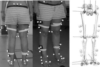
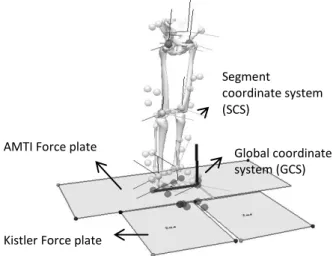
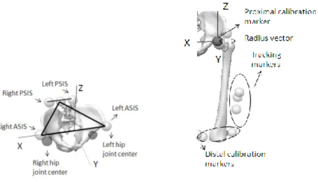
Figure 1 - Marker setup used for motion captures and lower limb and pelvis constructions: five markers for pelvis, five markers for thigh, seven markers for shank an eight markers for foot a) Posterior setup. b) Anterior setup. c) Reconstructed biomechanical model in Visual 3-D. ... 31 Figure 2 - Static trial to set all the segments as a reference position and to model construction based on the marker setup, in Visual 3-D. Subject was located near to the Laboratory or Global Coordinate System (LCS), on the calibrated volume. .... 32 Figure 3 - a) CODA model and for pelvis construction in Visual 3-D: ASIS and PSIS are

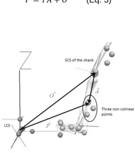
necessary to determine pelvis SCS. b) Setup for body segments construction, using the distal and proximal markers and tracking markers, which let the segment follow its coordinates... 33 Figure 4 - Determination of A point from measurement of P in SCS regarding the

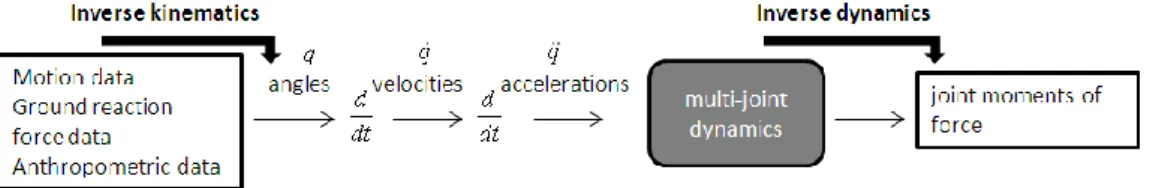
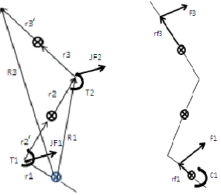
transformation matrix T and the translation O. LCS is the laboratory coordinate system or global coordinate system (GCS). Model reconstructed in Visual3-D. ... 34 Figure 5 - Workflow of the inverse problem using inverse kinematic and dynamic solutions. ... 36 Figure 6 - a) Definition of vectors and location of center of mass, proximal forces and

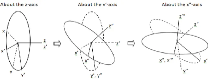
torques. b) Identification of external forces and couples. ... 37 Figure 7 - Cardan sequence for pelvis angles processing, Z-Y’-Z’’ (adapted from Ying &

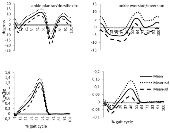
Kim, 2002). ... 38 Figure 8 - Mean and standard deviations curves of ankle range of motion - ROM

(above figures) in sagittal (left side) and frontal (right side) planes and the respective Mf (lower figures). ... 40

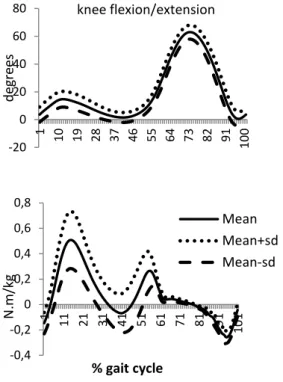
Figure 9 - Mean and standard deviations curves of knee ankle range of motion - ROM (above figure) in sagittal plane and the respective Mf (lower figure). ... 41

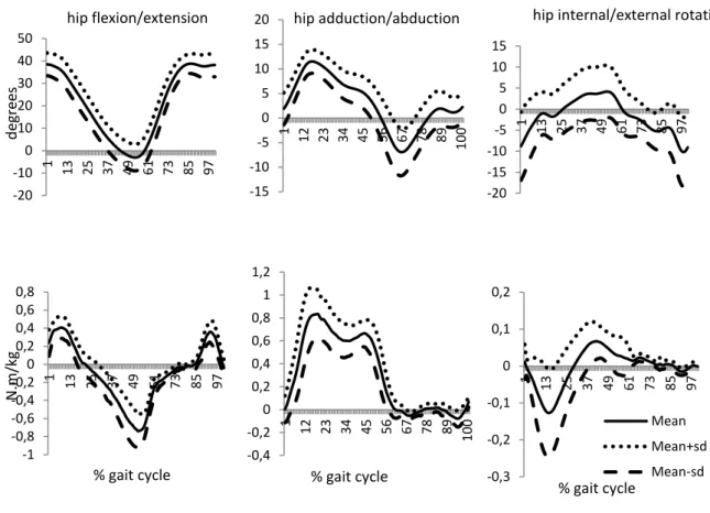
Figure 10 - Mean and standard deviations curves of hip range of motion - ROM (above figures) in sagittal (left side), frontal (middle) and transversal (right side) planes and the respective Mf (lower figures). ... 42

(18)

XVIII

Figure 11 - Mean and standard deviations curves of pelvis range of motion - ROM in sagittal (left side), frontal (middle) and transversal (right side) planes. ... 43 Figure 12 - Ankle, knee and hip joints range of motion (ROM) in sagittal (first row),

frontal (second row) and transversal planes (third row) for the non-pregnancy (NP), pregnancy (PG) and load carrying (LCG) groups. ... 59 Figure 13 - Pelvis range of motion (ROM) in sagittal (first row), frontal (second row) and transversal planes (third row) for the non-pregnancy (NPG), pregnancy (PG) and load carrying (LCG) groups. ... 59 Figure 14 – Ankle, knee and hip joints moments of force (Mf) in sagittal (first row),

frontal (second row) and transversal planes (third row) for the non-pregnancy (NPG), pregnancy (PG) and load carrying (LCG) groups. ... 60 Figure 15 – Ankle, knee and hip joints moments of force (Mf) in sagittal (first row),

frontal (second row) and transversal planes (third row) for the non-pregnancy (NPG), pregnancy (PG) and load carrying (LCG) groups. ... 61 Figure 16 - Marker setup used for motion captures and lower limb and pelvis constructions: five markers for pelvis, five markers for thigh, seven markers for shank an eight markers for foot a) Posterior setup. b) Anterior setup. c) Reconstructed biomechanical model in Visual 3-D. ... 74 Figure 17 - In the same frame of the same cycle d1, d2 and d3 are the differences between three markers associated to a segment, calculated with 6 degrees of freedom (6DOF) and global optimization model (GOM) approaches. ... 77 Figure 18 - Ankle, knee and hip joints and pelvis range of motion (ROM) in sagittal (first

column), frontal (second column) and transversal planes (third column) for the non-pregnant group (NPG). The solid line represents the 6 degrees of freedom (6DOF) model; the round dot line the Universal-Revolute-Spherical (URS) model, the square dot the Spherical-Revolute-Spherical (SRS) model; and the dash line the Spherical- Spherical-Spherical (SSS) model. ... 85 Figure 19 - Ankle, knee and hip joints and pelvis range of motion (ROM) in sagittal (first column), frontal (second column) and transversal planes (third column) for the pregnant group (PG). The solid line represents the 6 degrees of freedom (6DOF) model; the round dot line the Universal-Revolute-Spherical (URS) model, the square dot the Spherical-Revolute-Spherical (SRS) model; and the dash line the Spherical- Spherical-Spherical (SSS) model. ... 86 Figure 20 - Plug-in-Gait Marker Placement Protocol. ... 96 Figure 21 - Foot segment, represented as a rigid body. ... 98 Figure 22 - Representation of the closed-loop feedback control system to optimize the

(19)

XIX

Figure 23 - Ground reaction forces curves, of the collected experimental and simulated data, for all the subjects and regarding the four moments: first trimester (1T), second trimester (2T), third trimester (3T) and post-partum (PP). The dashed line represents the experimental data. The solid line represents the simulation data. ... 104

(20)

XX

List of Abbreviations

 1T – First trimester  2T – Second trimester  3-D - Three dimensional  3T – Third trimester

 6DOF - Six degrees of freedom

 ASIS - Anterior superior iliac spine

 BMI - Body Mass Index

 DLST - Double limb support time

 DOF - Degrees of freedom

 F1 – Loading response peak force

 F2 – Mid stance response peak force

 F3 – Terminal stance response peak force

 GCS - Global Coordinate System

 GOM - Global Optimization Method

 GRF - Ground Reaction Forces

 IOM - Institute of Medicine

 ISAK - International Society for the Advancement of Kinanthropometry

 LCG - Load carrying group

 SCS - Segment Coordinate System

 LCS - Laboratory Coordinate System

 LHJC - Left hip joint center

 Me – Median

 Mf – Moments of force

 NPG_LCG – Comparison between non-pregnant and load carrying groups

 NPG_PG - Comparison between non-pregnant and pregnant groups

 NPG – Non-pregnant group

 NRC - American Research Council

 PD - Proportional-derivate

 P – Pregnancy

 PG_LCG – Comparison between pregnant and load carrying groups

 PG - Pregnant group

 PP – Post-partum

 PSIS - Posterior superior iliac spine

 PW - Pregnant women

 RHJC - Right hip joint center

 RHS - Right heel strike

 ROM - Range of motion

 RTO - Right toe off

 SCS - Segment coordinate system

 SP - Stance phase

 SRS - Spherical-Revolute-Spherical

 SSS - Spherical-spherical-spherical

 STA - Soft tissue artifact

 SW – Swing phase

(21)

21

Chapter

1

(22)

22

1.1 Rationale for the Investigation

One of the most studied human movements is gait, once it is the basic mean of locomotion and it is used throughout the life. Thus, since childhood to elderly, walking is the functional way of moving from one place to another. With growing, the human body will change anatomically, going through different stages of growth and in adulthood there is a possible stabilization of its development.

The musculoskeletal system is constantly subjected to mechanical loading which is a prerequisite for morphological and functional adaptations of biological materials. Bones, cartilages, ligaments and tendons have some stress and strain limits and once they are exceeded, micro and macro damages can occur. Pain and injuries have relation with overloading conditions, and as a bionegative response, this situation can cause loss of strength and function. On the other side, biological structures need mechanical stimulus to maintain or increase their function capacity and morphological structure (Brüggemann, 2005).

The human body weight is an anthropometric variable crucial to the amount of load that the body supports static and dynamically. Excessive body weight is related to several health problems and gait related injuries (Must & Strauss, 1999). Pregnancy is a special phase of life and also an overweight condition, with some specific associated health problems caused by the morphological, physiological and hormonal changes (Nicholls & Grieve, 1992). When walking the human body can adjust to different circumstances thereby changing the gait pattern. Muscle function can be reorganized to provide body acceleration and therefore modify the gait pattern, which may add an overload to the musculoskeletal system (Foti, Davis & Bagley, 2000). The assessment of biomechanical loading in the musculoskeletal system of the pregnant women is of particular interest since it is important to better understand the gait adaptations during pregnancy and few biomechanical studies can be found in literature

Moreover, it is important to quantify the biomechanical load and the musculoskeletal adaptations that occur during gait and identify which ones are more related with the increased trunk mass, or which ones can be more associated to physiological and hormonal changes. This analysis can provide more information about joint loads and kinematics and it may be useful to exercise prescription in order to reduce the risk of discomfort or injure associated to overload.

(23)

23

The changes associated to pregnancy as weight gain, skinfolds increase, increased ligamentous laxity, decreased neuromuscular control and coordination and swelling of the arms and legs (Pitkin, 1976; Taggart, Holliday, Billewicz, Hytten & Thomson, 1967; Butte, Ellis, Wong, Hopkinson & Smith, 2003; Block, Hess, Timpano & Serlo, 1985; Brett & Baxendale, 2001; Calganeri, Bird & Wright, 1982; deGroot, Adam & Hornstra, 2003; Dumas, Reid, Wolfe, Griffin & McGrath, 1995; Dunning et al., 2003; Hainline, 1994; McNitt-Gray, 1991; Snijders, Seroo, Snidjer & Hoedt, 1976) may contribute to the increase of the soft tissue artifact (STA). This can be a concern for biomechanical modeling, where the efficacy of gait analysis information may be restricted by sources of error like the soft tissue displacement relative to bone. So, there is the need to obtain accurate data on gait analysis, particularly regarding overweight conditions related to pregnancy. The global optimization method proposed by Lu and O'Connor (1999) estimates the general pose for each frame, by minimizing the differences between the measured coordinates in the static position and the measured coordinates during motion in order to find an optimal position for the set of segments. To minimize the STA effect in pregnant women, the GOM can be applied, where joint constraints are added to the model in order to minimize the sensor noise and estimate an optimal pose of a multi-link model that best matches the motion capture data in terms of global criterion (Lu & O'Connor, 1999).

Typically, the gait cycle is defined as the amount of time from the initial foot contact with the ground to the next instant when the same foot starts the following initial contact (Peterson & Bronzino, 2008). As a cyclical locomotor task, gait provides several impacts on the ground. Ground reaction forces produces joint reaction and moments of force, and some internal forces as bone-on-bone, ligament and muscle forces (Winter, 2009). To analyze human gait, ground reaction forces (GRF) and motion data are measured. Both parameters are used to calculate other variables, as joint moments which are calculated by the inverse dynamics method and add more information about the stress imposed in the joints and the necessary muscle control (Perry, 1992). Also, the GRF are a common indicator for external biomechanical load. When GRF are unobtainable, simulation models can predict these data and can add more information for the understanding of interactions of the musculoskeletal system with the physical environment, such as the foot floor contact. In a clinical context, applied to pregnant population, this methodology can be important to provide more important biomechanical information that could not be collected in another way and to monitoring the foot contact during the pregnancy.

(24)

24

1.2 General Research Questions

Walking is the primary mean of human locomotion and gait analysis is useful to quantitative measurement and assessment (Peterson & Bronzino, 2008). But throughout life, human body can adjust to different conditions and the gait pattern may change. During pregnancy, women are subject to morphological, physiological and hormonal changes, which can lead to adaptations in gait. It is important to quantify the internal and external biomechanical load related to pregnancy condition and to clarify which gait adaptations are more related with the increased trunk mass, or which can be more associated to physiological and hormonal changes.

Also, considering the pregnancy condition, there is a possibility of a higher STA and to minimize the associated error there is the need to use the GOM to obtain a more accurate three-dimensional (3-D) multibody biomechanical gait model that best represents the pregnant women.

In order to obtain all the variables, two solutions will were used: inverse and forward dynamics.

1.3 Purposes of the Thesis

The purposes of the present thesis were to:

1) Develop a 3-D biomechanical model of the lower limb, based on a rigid multibody system;

2) Describe the angular kinematics of the lower limb of young and pregnant women and women carrying an extra load;

3) Calculate net moments of force in ankle, knee and hip joints, using inverse dynamics;

4) Describe peak magnitudes of the joint moments of force of young and pregnant women and women carrying an extra load;

5) Determine the temporal parameters of the gait cycle of young and pregnant women and women carrying an extra load;

6) To identify potential differences between the three groups on the biomechanical parameters, concerning gait cycle;

7) To use three different constraining sets in the lower limb joints, in pregnant and non-pregnant women biomechanical models. The ankle, knee and hip joints

(25)

25

were modeled respectively with the following characteristics: 1) universal-revolute-spherical, 2) spherical-revolute-spherical and 3) spherical-spherical-spherical;

8) To use simulation technique to predict vertical ground reaction forces generated during gait in pregnant women.

1.4 Thesis Overview

Following the present introduction (chapter 1), this thesis embraces a compilation of four papers, as follows.

The aim of the first study (chapter 2) was to describe the gait pattern during the second trimester of pregnancy and give an orientation for biomechanical modeling of the lower limb of pregnant women. This model construction revealed to be appropriate to describe gait during second trimester of pregnancy.

The aim of the second study (chapter 3) was to analyze the effect of the increased mass in the trunk associated to pregnancy on the lower limb and pelvis, during walking task, on temporal-distance parameters, joint range of motion (ROM) and moments of force (Mf), by comparing second trimester pregnant women group to non-pregnant

women group.

The aim of the third study (chapter 4) was to compare three different approaches on joint modelling of the ankle, knee and hip, as follows: 1) universal-revolute-spherical (URS); 2) spherical-revolute-spherical (SRS), and; 3) spherical-spherical-spherical (SSS), in regard of the gait of two groups of participants: 1) second trimester pregnant women, and; 2) non pregnant women.

The aim of the fourth study (chapter 5) was to predict vertical ground reaction forces (GRF) generated during gait, measured in the three trimesters of pregnancy and post-partum, by means of a contact model (simulation).

Finally, in chapter 6, a general discussion and main conclusions of the thesis are presented, as well as few recommendations for future research.

The study was approved by ethics committee of Faculty of Human Kinetics, University of Lisbon.

(26)

26

1.5 References

Block, R.A., Hess, L.A., Timpano, E.V. & Serlo, C., (1985). Physiological changes in the foot in pregnancy. Journal of the American Podiatric Medical Association, 75, 297–299.

Brett, M. & Baxendale, S., (2001). Motherhood and memory: a review. Psychoneur- oendocrinology 26, 339–362.

Brüggemann, G.P. (2005). Mechanical Loading of Biological Structures and Tissue Response. In Rodrigues, H; Cerrolaza, M; Doblaré, M; Ambrósio, J & Viceconti, M (Eds), Proceedings of the ICCB 2005 – II International Conference on Computational Bioengineering, 1-2,25-26.

Butte, N., Ellis, K., Wong, W., Hopkinson, J. & Smith, E. (2003). Composition of gestational weight gain impacts maternal fat retention and infant birth weight. American Journal of Obstetrics and Gynecology, 189(5), 1423-1432.

Calganeri, M., Bird, H.A. & Wright, V. (1982). Changes in joint laxity occurring during pregnancy. Annals of the Rheumatic Diseases, 41, 126–128.

de Groot, R.H., Adam, J.J. & Hornstra, G. (2003). Selective attention deficits during human pregnancy. Neuroscience Letters, 340, 21–24.

Dumas, G.A., Reid, J.G., Wolfe, L.A., Griffin, M.P. & McGrath, M.J. (1995). Exercise, posture, and back pain during pregnancy. Clinical Biomechanics, 10, 98–103. Dunning, K., LeMasters, G., Levin, L., Bhattacharya, A., Alterman, T. & Lordo, K.

(2003). Falls in workers during pregnancy: risk factors, job hazards, and high risk occupations. American Journal of Industrial Medicine, 44, 664–672.

Foti, T. ; Davids, J. & Bagley, A. (2000). A Biomechanical Analysis of Gait During Pregnancy. The Journal of Bone and Joint Suergery, Incorporated, 82-A(5), 625-632.

Hainline, B. (1994). Low back pain in pregnancy. Advances in Neurology, 64, 65–76. Lu, T.W. & O'Connor, J.J.(1999). Bone position estimation from skin marker

coordinates using global optimization with joint constraints. Journal of Biomechanics, 32, 129-134.

McNitt-Gray, J.L. (1991). Biomechanics related to exercise in pregnancy, Exercise in pregnancy 2nd edition Williams & Wilkins, Baltimore 133-140.

Must, A. & Strauss, R. (1999). International Journal of Obesity and Related Metabolic Disorders, 23,S2-11.

Nicholls, J.A. & Grieve D.W. (1992). Performance of Physical Tasks in Pregnancy. Ergonomics, 35,301-11.

Perry, J. (1992) Gait Analysis. Normal and Pathological Function. Thorofare, New Jersey: SLACK Inc.

Peterson, D.R. & Bronzino J.D. (2008). Biomechanics: Principles and Applications (2nd ed.). Boca Raton: CRC Press.

Pitkin, R. (1976). Nutritional support in obstetrics and gynecology. Clinical Obstetrics and Gynecology, 19(3), 489 – 513.

Snijders, C.J., Seroo, J.M., Snijder, J.G. & Hoedt, H.T. (1976). Change in form of the spine as a consequency of pregnancy. In: Proceedings for the 11th International Conference on Medical and Biological Engineering. 670-671. Ottawa, ONT, CAN. Taggart, N., Holliday, R., Billewicz, W., Hytten, F. & Thomson, A. (1967). Changes in

skinfolds during pregnancy. British Journal of Nutrition, 21(2), 439-451.

Winter, D.A. (2009). Biomechanics and Motor Control of Human Movement (4th ed.). New Jersey: John Wiley & Sons.

(27)

27

Chapter

2

2 Biomechanical Model for Kinetic and

Kinematic Description of Gait During

Second Trimester of Pregnancy to Study

the Effects of Biomechanical Load on the

Musculoskeletal System

1

Published as: Aguiar L, Santos-Rocha R, Branco M, Vieira F, Veloso AP (2014). Biomechanical model for kinetic and kinematic description of gait during second trimester of pregnancy to study the effects of biomechanical load on the musculoskeletal system. Journal of Mechanics in Medicine and Biology (JMMB), 14, 1450004. DOI: 10.1142/S0219519414500043 (Appendix 2)

(28)

28

2.1 Abstract

Walking is daily physical activity and a common way of exercise during pregnancy, but morphological changes can modify the gait pattern. Biomechanical models can help in evaluating joint mechanical loads, kinetics and kinematics during gait and provide the knowledge about the pattern of movement. This study aims to describe the gait pattern during the second trimester of pregnancy and give an orientation for biomechanical modeling of the lower limb of pregnant women. An inverse dynamics three-dimensional approach was used. Ankle and hip joint seem to be more overloaded, mainly in the sagittal and frontal plane, respectively. Results showed that pregnant women have a similar walking pattern to the normal gait. This model construction revealed to be appropriate to describe gait during the second trimester of pregnancy.

(29)

29

2.2 Introduction

Locomotor system models are an increasingly common way of studying human gait and a variety have been developed to perform specific functions (Zajac, Neptune & Kautz, 2002; 2003) and specific conditions. Human body can adjust to different conditions and the gait pattern may change. Muscle function may be reorganized to provide body acceleration and therefore modify the gait pattern, which contribute to an overload on the musculoskeletal system, causing discomfort and even pain in lower back, hip and leg (Foti et al., 2000).

During pregnancy, women are subject to morphological, physiological and hormonal changes, which can lead to adaptations in gait. These changes can include weight gain, swelling of the arms and legs, increased ligamentous laxity, decreased neuromuscular control and coordination, decreased abdominal muscle strength, increased spinal lordosis, altered biomechanical parameters, an anterior displacement in the location of the center of mass, and changes in mechanical loading and joint kinetics (Block et al., 1985; Brett & Baxendale, 2001; Calganeri et al., 1982; deGroot et al., 2003; Dumas et al., 1995; Dunning et al., 2003; Hainline, 1994; McNitt-Gray, 1991; Snijders et al., 1976). Other studies demonstrated that more than 50% of women reported swelling of the foot, ankle, and leg, unsteady gait, increased foot width and hip pain (Ponnapula & Boberg, 2010). From week 20th changes due to pregnancy, as weight gain and skinfolds increase, are already well established and are clearly visible (Pitkin, 1976; Taggart et al., 1967; Butte et al., 2003). In what concerns weight gain, according to the Institute of Medicine (IOM) and the National Research Council (NRC) (2009) recommendations, the body mass of a woman with avarage body mass index (BMI) may increase between 11.5 and 16 kg.

Foti et al. (2000), used three-dimensional (3-D) motion data of 15 women during the end of the third trimester, and again one year after delivery. Kinematic and kinetic parameters were compared between the two conditions. It was found that the gait pattern was remarkably changed during pregnancy. Concerning kinetic parameters, it was observed an increase in the hip moment and power in the frontal and sagittal planes. The general pattern of gait kinematics in pregnant women is similar to that of no pregnant women, however, at faster speed, pregnant women have difficulty in coordinating between the thorax and pelvis. Pregnant women prefer to walk with slower speed, but this fact cannot be explained as energy economy mode, since walk more slowly than the comfort speed, requires more energy (Wu et al., 2004).

(30)

30

Walking is daily physical activity and a common way of exercise during pregnancy, but morphological changes can modify the gait pattern. Biomechanical models can help in evaluating joint mechanical loads, kinetics and kinematics during gait and provide the knowledge of the movement patterns. However, such modifications may become a concern in biomechanical models construction. Joint centers are calculated based on the marker’s locations and the swelling of the segments may increase the error associated with the marker placement. In the pelvis, marker locations have special attention due the mass distribution in the anterior trunk moving forward the position of the center of mass. Another concern is to minimize soft tissue artifact produced by segments mass vibration.

2.3 Objectives

This study aims to describe the gait pattern during the second trimester of pregnancy and give an orientation for 3-D biomechanical modeling of the lower limb of pregnant women.

2.4 Materials and Methods

Some methodological problems may be associated with the kinematic and kinetic variables estimations due to anthropometric characteristics as marker locations for three-dimensional segments reconstruction and markers associated to skin movement. The aim of the present is to contribute to add more information to biomechanical gait analysis regarding the specific conditions of pregnancy, provided by a 3-D biomechanical model constructed based on two main processes: inverse kinematics and inverse dynamics methods.

2.4.1 Subjects

Eighteen pregnant women (PW) with 27.3 weeks (second trimester) mean gestational age, mean chronological age of 32.6 years, 68.2 kg of weight, 1.60 m of height and mean BMI of 26.3 kg/m2 (table 1), participated in this study.

(31)

31

Table 1 - Characterization of sample group (mean ± standard deviation): age, weight, height, body mass index (BMI) and gestational age.

2.4.2 Data Collection and Processing

Anthropometric data (weight and height) were collected following ISAK recommendations, to calculate de body segments masses and inertia moments. Reflective spherical markers were placed on anatomical points according to the defined marker setup protocol (figure 1). Motion capture was performed with an optoelectronic system of twelve cameras Qualisys (Oqus-300) operating at a frame rate of 200 Hz, synchronized with two force platforms (Kistler AG, Winterthur, Switzerland) and one AMTI (Advanced Mechanical Technology, Inc, Watertown, MA), which collected ground reaction force (GRF) data. The participants walking during three non-consecutive minutes at a comfortable speed, with a break of thirty seconds between each trial.

Figure 1 - Marker setup used for motion captures and lower limb and pelvis constructions: five markers for pelvis, five markers for thigh, seven markers for shank an eight markers for foot a) Posterior setup. b) Anterior setup. c) Reconstructed biomechanical model in Visual 3-D.

Age (years) Weight (kg) Height (m) BMI (kg/m2₎ Gestational age (weeks) PW 32.6±2.7 68.2±7.3 1.6±0.1 26.3±2.6 27.3±3.0

(32)

32 Segment coordinate system (SCS) Global coordinate system (GCS) AMTI Force plate

Kistler Force plate

Gait cycles were selected based on the force platforms and on the quality of both GRF. Cycle started at the right heel strike (RHS) and finished at the next RHS.

A static trial was performed (figures 1 and 2) which enables segments reconstruction and allows scaling the model, defining of the joint centers and the segment coordinate system (SCS) (figure 2).

Figure 2 - Static trial to set all the segments as a reference position and to model construction based on the marker setup, in Visual 3-D. Subject was located near to the Laboratory or Global Coordinate System (LCS), on the calibrated volume.

To create the local SCS it was necessary to establish the frontal plane using border targets: medial-distal, medial-proximal, lateral-distal and lateral-proximal. The SCS was created using the midpoints between the medial and lateral targets to define the distal and proximal end points. The SCS Z-axis was determined by the unit vector directed from the distal segment end point to the proximal segment end. The SCS Y-axis was determined by the unit vector that is perpendicular to both the frontal plane and the Z axis. Finally, the SCS X-axis was determined by the application of the vector product and as consequence using the right hand rule. The SCS Z-axis is directed from distal to proximal, the SCS Y-axis is directed from posterior to anterior, and the SCS X-axis is medial-lateral in orientation. For the pelvis, the (x-y) plane of the segment coordinate system is defined as the plane passing through the right and left ASIS (anterior superior iliac spine) markers, and the mid-point of the right and left PSIS (posterior superior iliac spine) markers.

Segments were defined using a proximal and a distal end point, measured by the middle distance between lateral and medial markers. Foot segment was defined by first

(33)

33

and fifth metatarsals lateral and medial tibia malleolus. For the shank it was used markers placed in tibia malleolus and in femur condyles. Pelvis was built based on CODA model (figure 3a), defined using the anatomical locations of the right and left ASIS and the right and left PSIS. This model allows the estimation of the right and left hip joint center (LHJC; RHJC) using the regression equation (equations 1 and 2) proposed by Bell, Pedersen and Brand (1989, 1990).

RHJC = (0.36 ∗ ASIS_Distance, −0.19 ∗ ASIS_Distance, −0.3 ∗ ASIS_Distance) (Eq. 1) LHJC = (−0.36 ∗ ASIS_Distance, −0.19 ∗ ASIS_Distance, −0.3 ∗ ASIS_Distance) (Eq.2)

Tracking markers (figure 3b) were also used allowing the segment to follow their coordinates to replicate the performed motion. In the foot, markers were placed in the second metatarsal, lateral side and in the heel, and a three marker cluster was strapped around the leg and another one around the thigh. In the pelvis, it was added a marker placed in the middle point between the PSIS markers to ensure at least three tracking markers.

Figure 3 - a) CODA model and for pelvis construction in Visual 3-D: ASIS and PSIS are necessary to determine pelvis SCS. b) Setup for body segments construction, using the distal and proximal markers and tracking markers, which let the segment follow its coordinates.

The position and orientation of the local SCS is described with respect to the laboratory coordinate system (LCS) (figure 4). The location of one point in the LCS is given by equation 3, where T is the rotation matrix from the SCS to the LCS and O is the translation between coordinate systems.

(34)

34

𝑃 = 𝑇𝐴 + 𝑂 (Eq. 3)

Figure 4 - Determination of A point from measurement of P in SCS regarding the transformation matrix T and the translation O. LCS is the laboratory coordinate system or global coordinate system (GCS). Model reconstructed in Visual3-D.

Thus, A is a point determined from measurement of P at this position (equation 4). The matrix T and translation vector O, are computed in all instants, provided that for at least three noncolinear points and can be found by minimizing the sum of squares error (equation 5), under the orthonormal condition (equation 6), where m is equal to the number of targets on the segment. Langrange multipliers are used, to find the maxima and minima of the function subject to constraints, given by equation 7 (Spoor & Veldpaus, 1980). 𝐴 = 𝑇−1_{(𝑃 − 𝑂) (Eq. 4)} ∑𝑚 ((𝑃_𝑖− 𝑇𝐴_𝑖) − 𝑂)2 𝑖=1 (Eq. 5) 𝑇−1_{𝑇 = 𝑇}𝑇_{𝑇 = 𝐼 (Eq. 6)} 𝑔(𝑇) = 𝑇𝑇_{𝑇 − 𝐼 = 0 (Eq. 7)}

All the markers coordinate data were interpolated using third degree polynomial to fulfill gap displacements. To reduce the noise the motion data was filtered, using a low pass Butterworth filter, with a cutoff frequency of 15 Hz (Winter, 1991). Each marker location was recognized in the static collection, which is as a reference position and must be set in each frame.

(35)

35

Due to the skin movement, the markers move relatively to the bone, modifying the initial configuration and therefore reproducing noisy motion data. Moreover, the segments are considered linked rigid bodies and joints have six degrees of freedom (6DOF), making them independent from each other and allowing more movement. Joint degrees of freedom were manipulated through the Inverse Kinematics tool in order to achieve the kinematic that can reproduce better the real motion. The inverse kinematics is based on the method of global optimization (Lu & O'Connor, 1999) and allows finding an optimal position for the set of segments, which constitute the model on each frame, the differences between the measured coordinates in the static position and the motion measured coordinates are minimized by the method of least squares. Thus, in the ankle, rotations in sagittal and frontal plane were allowed (universal joint), in the knee only the sagittal rotation was unrestricted (revolute joint) and in the hip all the rotations were used (spherical joint). Translations were locked for the three joints. These were the default available degrees or freedom provided by the software Visual 3-D C-Motion, Inc. Frame by frame, the recorded motion reproduces the model joint angles set in a configuration that best represents the experimental kinematics.

Given a set of measured marker coordinates P on a data frame, the global optimization is to find a set of generalized coordinates  so that the following error function (equation 9) is minimized, where W is a positive-definite weighting matrix, P’() is the corresponding set of marker coordinates calculated by the transformation given by equation 8, from the segment frame to laboratory frame.

P′₍__{) = T(}__)P∗_{(Eq. 8)}

T() is the transformation matrix from the SCS to LCS. This condition also maintains the rigid body condition and the integrity of the model once joint constraints are part of the model.

𝑓() = [𝑃 − 𝑃′₍__)]𝑇_{𝑊[𝑃 − 𝑃}′₍__{)] (Eq. 9)}

W is a (3mi x 3mi) weighting matrix (equation 10) assigned to the each segment to

reflect the error distribution among the mi markers. To each segment is given different

weighting factor reflecting its average degree of soft tissue artifacts. In this study it was used 1 for all segments weights.

𝑊 = [ 𝑊0 0 0 0 0 𝑊1 0 0 0 0 ⋱ 0 0 0 0 𝑊𝑛 ] (Eq. 10)

(36)

36

For each segment, the equation 11 is solved to find the minimum value, under the orthogonal constrain RT_{R = I, where x}

i and yi are position vectors of marker i at the

reference and global positions, respectively. R is the rotation matrix, v is the translation vector and m is the number of markers.

𝑓 = ∑𝑚𝑖=1(𝑅𝑥𝑖+ 𝑣 − 𝑦𝑖)𝑇(𝑅𝑥𝑖+ 𝑣 − 𝑦𝑖) (Eq. 11)

The minimum value of f is the segmental residual error (e), a measure of the markers distortion which is mainly due to soft tissue artifacts. The weighting matrix Wi is defined

as equation 12.

𝑊𝑖 =_𝑒1

𝑖𝐼 (Eq. 12)

This calculation is proposed for the kinematics of a rigid body between two sequential positions, where the first one works as the reference (Cappello, Francesco, Palombara & Leardini, 1996; Challis, 1995; Spoor & Veldpaus, 1980). The segments velocities and accelerations were obtained by derivation of the new position equations.

The inverse dynamics method = 𝐼𝐷(𝑚𝑜𝑑𝑒𝑙, 𝑞, 𝑞,̇ 𝑞̈) (figure 5) was used to calculate the forces and moments produced by the muscular action, requiring the estimated mass and inertia values, body segments linear and angular accelerations, as the data from external forces measured by the force plates. The weights and locations of the centers of mass for each body segments considered were calculated using the regression equations of Dempster and inertia moments using inertial properties based on their shape (Hanavan, 1964). To determine the joints net moments and forces, the equations of motion was iteratively solved, considering the equilibrium dynamic and boundary conditions.

Figure 5 - Workflow of the inverse problem using inverse kinematic and dynamic solutions.

The joint torques calculation was performed during the right foot stance phase from the heel strike (heel touches the ground) to toe off (foot leaves of the ground), completing approximately 60% of gait cycle. The cycle starts with the left foot contact with the platform and ends in the next heel contact of the same foot with the ground.

(37)

37

As figure 6 shows, the first step is defining the location of the center of mass of each segment to identify the position vectors relatively to the SCS given by the vectorial summation (equation 13).

𝑅_𝑖 = 𝑟_𝑖+ 𝑟_𝑖′_{+ 𝑟}

𝑖−1 (Eq. 13)

Then, we must identify the proximal forces and torques due to inertia and joints and finally include external forces and couples (figure 6).

Figure 6 - a) Definition of vectors and location of center of mass, proximal forces and torques. b) Identification of external forces and couples.

The proximal joint reaction force is computed in the global coordinate system (GCS), using an iterative algorithm, which allows any applied external force on segments (equation 14), where mi is the mass of segment i, ai is the acceleration of segment i, n

the number of distal segments connected in chain, q the number of external forces and Fq, the applied external forces.

𝐹_{𝑝𝑟𝑜𝑥𝑖𝑚𝑎𝑙} = ∑𝑛𝑖=1𝑚_𝑖(𝑎𝑖+ 𝑔) + ∑𝑞𝑗=1𝐹𝑞 (Eq. 14)

The proximal moment due to the inertial forces and applied moments at the joint is calculated by equation 15, where Pj is the vector from application of the external force

to the proximal joint, p is the number of external couples (), Ri is the distance from

center of gravity of each distal segment to proximal joint, 𝐴_𝑖 = 𝑚_𝑖(𝑎_𝑖+ 𝑔) and 𝐶_𝑖 = 𝑇−1_𝐶

𝑖′. 𝑇 is the matrix that transforms inertial torque form SCS to LCS based on the motion data.

𝑀𝑝𝑟𝑜𝑥𝑖𝑚𝑎𝑙 = ∑𝑛𝑖=1(𝐶𝑖+ 𝑅𝑖𝐴𝑖) + ∑𝑞𝑗=1(𝑃𝑗𝐹𝑞) + ∑𝑝𝑘=1𝑘 (Eq. 15)

(38)

38

𝑀_𝑖 = 𝐶_𝑖+ 𝐶_𝑖−1+ 𝑟_𝑖× 𝐹_𝑖+ 𝑟_𝑖′_{× 𝐹}

𝑖−1 (Eq. 16)

Is important to remember that the T matrix, transforms the inertial torque Ci’ from the

SCS into Ci in the LCS. So, the proximal couple is computed at the proximal end of a

segment in SCS is given by equation 17, where Ii is the inertia moment of the segment, α is the angular acceleration and ω is the angular velocity for the angular moment calculation 𝐼_𝑖𝜔_𝑖′_{(Siegel, Kepple & Stanhope, 2004).}

𝐶_𝑖′ _{= 𝐼}

𝑖𝛼𝑖′ + 𝜔𝑖′(𝐼𝑖𝜔𝑖′) (Eq. 17)

Joint angles and moments of force (Mf) were calculated in order to a SCS, using a

Cardan sequence of rotations x-y-z, for the ankle, knee and hip (Cole, Nigg, Ronsky, & Yeadon, 1993). However, as Baker (2001) suggested, pelvis angles were computed using z-y-x rotation to descript the movement relatively to the laboratory, representing axial rotation, obliquity and tilt (figure 7).

Figure 7 - Cardan sequence for pelvis angles processing, Z-Y’-Z’’ (adapted from Ying & Kim, 2002).

For ankle, shank and thigh segments x rotation was around the medial-lateral axis, y was related with anterior- posterior axis and z was around the vertical axis. Based on this sequential rotations, T matrix is (equation 18):

𝑇 = [

𝑐𝑜𝑠𝛽𝑐𝑜𝑠𝛾 𝑐𝑜𝑠𝛾𝑠𝑖𝑛𝛽𝑠𝑖𝑛𝛼 + 𝑠𝑖𝑛𝛾𝑐𝑜𝑠𝛼 𝑠𝑖𝑛𝛼𝑠𝑖𝑛𝛾 − 𝑐𝑜𝑠𝛼𝑠𝑖𝑛𝛽𝑐𝑜𝑠𝛾 −𝑠𝑖𝑛𝛾𝑐𝑜𝑠𝛽 𝑐𝑜𝑠𝛼𝑐𝑜𝑠𝛾 − 𝑠𝑖𝑛𝛼𝑠𝑖𝑛𝛽𝑠𝑖𝑛𝛾 𝑠𝑖𝑛𝛾𝑠𝑖𝑛𝛽𝑐𝑜𝑠𝛼 + 𝑐𝑜𝑠𝛾𝑠𝑖𝑛𝛼

𝑠𝑖𝑛𝛽 −𝑐𝑜𝑠𝛽𝑠𝑖𝑛𝛼 𝑐𝑜𝑠𝛼𝑐𝑜𝑠𝛽 ] (Eq. 18)

The T matrix as a final representation based on motion data is shown in equation 19:

𝑇 = [

𝑇11 𝑇12 𝑇13 𝑇21 𝑇22 𝑇23

(39)

39

Using both matrices (equations 18 and 19) it was possible to obtain the equations 20 to 22: 𝛽 = 𝑠𝑖𝑛−1_(𝑇 31) (Eq. 20) ∝= −𝑠𝑖𝑛−1₍𝑇32 𝑐𝑜𝑠𝛽) (Eq. 21) 𝛾 = −𝑠𝑖𝑛−1₍𝑇21 𝑐𝑜𝑠𝛽) (Eq. 22)

To calculate ankle, knee and hip joint angles and Mf, three-dimensional biomechanical

models were constructed, using the software Visual 3-D C-Motion, Inc.

2.4.3 Statistical Analysis

The results are based on five cycles per subject. Each cycle starts in the Right Heel Strike (RHS) and finish in the nest RHS. RHO and Right Toe Off (RTO) were created events to establish temporal-distance parameters. The average joint angles and moments curves were obtained for each participant as the mean curve for the group. Both angular displacement and Mf data were normalized to time cycle. The Mf were

normalized to body mass.

2.5 Results

2.5.1 Time and Distance Parameters

In what concerns to the temporal-distance variables, speed has a mean value of 1.16±0.12 m/s. Stride width was 0.10±0.02 m. Left and right step lengths were 0.62±0.05 with a duration of 0.54±0.03 s. Total cycle time was 1.07±0.06 s while left and right stance time were 0.65±0.04 s. Double limb support time was 0.22±0.03 s.

(40)

40

2.5.2 Kinematic and Kinetic Data

The range of motion (ROM) and Mf were analyzed according to the allowed degrees of

freedom. Maximum dorsiflexion and ankle plantar flexion angles were 12.16±3.05 and -14.34±5.10 deg, respectively. Sagittal ankle plane ROM was 26.50±3.65 deg. Peak ankle dorsiflexion Mf was 1.21±0.16 N.m/kg and the peak plantar flexion Mf was

-0.52±0.32 N.m/kg. In the frontal plane, maximum ankle eversion was -6.71±3.06 deg and maximum inversion was 7.18±3.49 deg; the correspondent ROM was 12.02±2.04 deg. Ankle eversion peak Mf was -0.05±0.02 N.m/kg and the inversion peak was

0.10±0.04 N.m/kg (figure 8).

Figure 8 - Mean and standard deviations curves of ankle range of motion - ROM (above figures) in sagittal (left side) and frontal (right side) planes and the respective Mf(lower figures).

In the knee joint, flexion maximum angle was 63.62±4.87 deg while the extension was -0.44±3.90 deg. In sagittal plane knee ROM was 64.06±5.39 deg. The peak flexion knee Mf was 0.53±0.20 N.m/kg and the peak extension Mf was -0.17±0.09 N.m/kg (figure 9).

-25 -20 -15 -10 -5 0 5 10 15 20 1 ₁₁ ₂₁ ₃₁ ₄₁ ₅₁ ₆₁ ₇₁ ₈₁ ₉₁ 101 d egre ss ankle plantar/dorsiflexion -15 -10 -5 0 5 10 15 1 ₁₀ ₁₉ ₂₈ ₃₇ ₄₆ ₅₅ ₆₄ ₇₃ ₈₂ ₉₁ 100 ankle eversion/inversion -0,2 0 0,2 0,4 0,6 0,8 1 1,2 1,4 1,6 1 ₁₁ ₂₁ ₃₁ ₄₁ ₅₁ ₆₁ ₇₁ ₈₁ ₉₁ 101 N .m/ kg % gait cycle -0,1 -0,05 0 0,05 0,1 0,15 0,2 1 ₁₀ ₁₉ ₂₈ ₃₇ ₄₆ ₅₅ ₆₄ ₇₃ ₈₂ ₉₁ 100 % gait cycle Mean Mean+sd Mean-sd

(41)

41

Figure 9 - Mean and standard deviations curves of knee ankle range of motion - ROM (above figure) in sagittal plane and the respective Mf(lower figure).

Maximum hip flexion reached 39.55±5.00 deg and maximum hip extension was -4.43±5.15 deg. Flexion/ extension hip ROM was 43.98±3.08 deg. Peak flexion and extension Mf were 0.43±0.09 N.m/kg and -0.79±0.18 N.m/kg, respectively. The mean

value of 11.92±2.38 deg was observed for hip maximum adduction and 7.77±4.95 deg for maximum abduction. The adduction/abduction ROM was 16.69±4.34 deg. Peak adduction Mf was 0.76±0.11 N.m/kg and peak abduction Mf (valley) was 0.52±0.09

N.m/kg. In the z axis, hip maximum internal rotation was 5.30±5.57 deg and maximum external rotation was -11.46±7.96 deg; the correspondent ROM was 16.76±5.36 deg. Peak internal rotation Mf was -0.12±0.05 N.m/kg and external peak Mf reached

0.08±0.04 N.m/kg (figure 10). -20 0 20 40 60 80 1 ₁₀ ₁₉ ₂₈ ₃₇ ₄₆ ₅₅ ₆₄ ₇₃ ₈₂ ₉₁ 100 d egre es knee flexion/extension -0,4 -0,2 0 0,2 0,4 0,6 0,8 1 ₁₁ ₂₁ ₃₁ ₄₁ ₅₁ ₆₁ ₇₁ ₈₁ ₉₁ 101 N .m/ kg % gait cycle Mean Mean+sd Mean-sd

(42)

42

Figure 10 - Mean and standard deviations curves of hip range of motion - ROM (above figures) in sagittal (left side), frontal (middle) and transversal (right side) planes and the respective Mf

(lower figures).

Maximum anterior pelvic tilt was 16.88±4.13 deg while maximum posterior pelvic tilt was 14.07±4.36 deg. Pelvic tilt ROM was 2.81±0.99 deg. In the frontal plane, maximum pelvic left and right obliquities were 7.13±2.15 deg and -6.39±3.16 deg, respectively. Pelvic obliquity ROM was 13.52±3.49 deg. Maximum transversal left rotation was 5.91±2.88 deg and right maximum rotation was -7.15±3.12 deg. Pelvic rotation ROM was 13.05±4.30 deg (figure 11).

-20 -10 0 10 20 30 40 50 1 ₁₃ ₂₅ ₃₇ ₄₉ ₆₁ ₇₃ ₈₅ ₉₇ d egre es hip flexion/extension -15 -10 -5 0 5 10 15 20 1 ₁₂ ₂₃ ₃₄ ₄₅ ₅₆ ₆₇ ₇₈ ₈₉ 100 hip adduction/abduction -20 -15 -10 -5 0 5 10 15 1 ₁₃ ₂₅ ₃₇ ₄₉ ₆₁ ₇₃ ₈₅ ₉₇

hip internal/external rotation

-1 -0,8 -0,6 -0,4 -0,2 0 0,2 0,4 0,6 0,8 1 ₁₃ ₂₅ ₃₇ ₄₉ ₆₁ ₇₃ ₈₅ ₉₇ N .m/ kg % gait cycle -0,4 -0,2 0 0,2 0,4 0,6 0,8 1 1,2 1 ₁₂ ₂₃ ₃₄ ₄₅ ₅₆ ₆₇ ₇₈ ₈₉ 100 % gait cycle -0,3 -0,2 -0,1 0 0,1 0,2 1 ₁₃ ₂₅ ₃₇ ₄₉ ₆₁ ₇₃ ₈₅ ₉₇ % gait cycle Mean Mean+sd Mean-sd

(43)

43

Figure 11 - Mean and standard deviations curves of pelvis range of motion - ROM in sagittal (left side), frontal (middle) and transversal (right side) planes.

2.6 Discussion

It was possible to observe similar angles and joint moment’s curves patterns as the maximum ROM and peak Mf values, compared with other studies related to pregnancy

(Foti et al., 2000). Concerning total gait cycle, stance phase was around 60% (Vaughan, Davis & O’Connor, 1992; Perry, 1992), similar to the normal gait pattern. In the ankle joint, the plantar flexion peak moment occurred during the early stance phase (figure 8). The dorsiflexor moment increased as the body moves in the forward direction. Peak inversion Mf increases in late stance phase.

Immediately after the first foot contact with the ground, there was a reaction vector anterior to the knee and hip joints, producing during the stance initial phase an extensor moment, which decreased with the alignment of this vector with the leg and thigh segments (Perry, 1992).

The hip peak flexion moment occurred in the beginning of the stance phase (while the extensor moment of the same joint, was recorded on the final stance phase. Adduction peak Mf revealed an higher value relatively to the other planes during the earlier stance

phase (figure 10). This can be related a larger base of gait during walking, which can improve locomotor stability (Foti et al., 2000; Bird, Menz & Hyde, 1999). Abduction peak moment was recorded in the middle of the stance phase. Internal and external peaks Mf registered lower values (figure 10).

Pelvic anterior tilt was maximum in the end of the stance phase, while left maximum obliquity was maximum in the earlier stance phase while right obliquity was maximum

0 5 10 15 20 25 1 ₁₃ ₂₅ ₃₇ ₄₉ ₆₁ ₇₃ ₈₅ ₉₇ d egre es % gait cycle pelvic tilt -15 -10 -5 0 5 10 15 1 ₁₃ ₂₅ ₃₇ ₄₉ ₆₁ ₇₃ ₈₅ ₉₇ % gait cycle pelvic obliquity -15 -10 -5 0 5 10 15 1 ₁₃ ₂₅ ₃₇ ₄₉ ₆₁ ₇₃ ₈₅ ₉₇ % gait cycle pelvic rotation Mean Mean+sd Mean-sd