Methodological aspects of a mathematical programming model to evaluate soil tillage technologies in a risky environment
Abstract
With this work we develop a methodology able to ensure the economic evaluation of soil tillage technologies, in a risky environment, and to capture the influence of farmer behaviour on his technological choice.
The model has short term activities, that change with the type of year and long term activities, in which the sets of traction investment activities are included. Although these activities do not change with the type of year, they lead to different availability of resources each type of year, since the same tractor has different available days to work in the field in different weather conditions.
We prove that the model is sensible to the grater income variability resulting from the use of alternative technologies and to the balance between income and risk, accounting to the probability of occurrence of each state of nature and giving an investment solution that considers each year the best production plan.
Keywords: Decision Analysis; Risk Management; Linear Programming; OR in agriculture;
1. Introduction
The aim of this work is to develop a methodology that is able to ensure the economic evaluation of soil tillage technologies, in a risky environment, and to capture the influence of farmer behaviour on his technological choice.
Alternative soil tillage technologies, namely direct seeding and reduced mobilization, can play an important role on the maintenance of farms competitiveness (Martins, 1994). In a risky environment the methodology used to the economic evaluation of alternative soil tillage technologies should incorporate in the analysis the grater inter-annual production variability of these technologies, when compared with traditional technology, and the inter-annual variability of the available days to perform the cultural operations needed to establish the cereals, since the available days are an important issue on the economic analysis of technologies and different types of years lead to different availability of days.
The farmer behaviour is another key issue. The income risk that tillage technologies have is due to production risk and to resources risk, given by the inter-annual variability on productions and available days. Farmers’ risk aversion may condition their technological option.
In this work, resources and productions variability’s are incorporated in a linear programming model. Carvalho (1994) refers that a huge number of studies at farm level, focused on farm planning in a risky environment, have been developed with the use of mathematical programming models, linear or not. Risk modelling techniques are built to produce a plan which, according to the producer preferences, maximizes his total satisfaction.
With mathematical programming it is possible to compare various technological options and consider the natural and economical factors influencing the technology use (Spharin & Seligman, 1983). The possibility of modelling the production system allows a set of efficient combinations of resources and products definition and the best selection (Boussard, 1971). Beside that, this method allows the system’s interactions consideration (Knipscheer et al., 1983).
2. The risk introduction on the technological economic evaluation problem
At farm level the income risk may affect the farm economical result expected value and the farmer options in what concerns the utilization of alternative farm tillage technologies.
The risk farmer faces in his farm may be due to environmental, political and institutional causes, depending on the use of production factors. The income risk comes from production risk, prices risk or resources risk that these causes imply simultaneously or not (Hardaker, et al., 1997, pág. 6).
Agricultural production is typically a risky activity and it is important to consider risk when planning a farm business. Costs and profits are influenced, during the production process, by the causes referred before, not controlled by farmer, and this affects the decisions at farm level – it is not expectable that farmers are pure profit maximizers (Carvalho, 1994).
Risk treatment in agriculture has been widely treated by several authors (Hazell & Norton, 1986; Rae, 1994, Hardaker, et al., 1997). Mathematical programming formulations use risk considering the stochastic parameters distribution is known. Once we know a probability distribution of the parameters the problem will be to represent this distribution inside the model structure (Carvalho, 1994).
The Expected Value/Variance model (Freund, 1956) brings the risk to the objective function, being used to generate the set of farm plans on the Expected Value/Variance frontier. This model can be linearly approximated using the MOTAD (Hazell, 1971), which doesn’t use the variance but the total absolute deviation, a linear estimator of variance, allowing the calculus of Risk/Income frontier by using linear programming.
The MOTAD model generates a Risk/Income frontier close to the Expected Value/Variance frontier but with slightly lower probability of containing the farmer’s expected utility maximizing solution (Hardaker et al, 1997).
The decision, according to these models, only depends on income average and variance, and the results assume a normal distribution.
Cocks (1968) suggested discrete stochastic programming model can give solutions to decision problems in which some of the technical coefficients and/or resources used can be well explained by a discrete probabilities distribution and Rae (1971) showed these models potential to solve stochastic decision problems.
3. Risk evaluation
Agricultural administration often requires that farmer take decisions without certain knowledge of these decisions’ implications. This way, many farms administration problems can be expressed by the decision theory since they involve the specification of possible actions, states of nature, states of nature probability of occurrence and an utility function to maximize (Rae, 1971).
Soil tillage technology choice represents a typical decision problem: the choice of optimal activities combination which differs among them in what concerns risk and expected income (Feder, 1980). So, the decision analysis in this context should be made using a method that allows the consideration of decision maker’s attitude to risk.
Decision theory is based on the subjective expected utility theory, which axioms have been specified by Bernoulli and, later, Von Neuman & Morgenstern.
A rational choice considering risk can be defined as a choice consistent with the decision maker’s beliefs about the chances of occurrence of alternative uncertain consequences and with his relative preferences for those consequences (Hardaker, et al., 1997, p. 29). The subjective expected utility theory is based exactly on these principles. The probabilities of occurrence of chance consequences reflect and quantify the decision maker expectations, while preferences translate his attitude to the consequences of the decision, i.e., to risk.
A risk averter decision maker will prefer less risky decision, which probability of occurrence of chance consequences that means significant losses is low, although the expected income is lower then the obtained with a riskier decision while a risk preferrer will prefer a risky decision even thought the occurrence probability of chance consequences giving significant returns is not high. Only a decision maker indifferent to risk will base is decision exclusively on expected income (Hardaker, et al., 1997, p. 87).
The problem of choice rationality considering risk in order to use the subjective expected utility theory is linked with the possibility of risk elements incorporation, related with uncertainty on resources availability and on the adjustment of input-output coefficients depending on the state of
nature. Considering this, the discrete stochastic programming model associated to a MOTAD structure suggested by Marques (1988) is the most suitable for the evaluation.
4. The farmer decision
Decision making is hardly neutral to risk and neglecting risk aversion in agricultural models can lead to an important overestimation of production levels and also influence farmer behaviour through proposed new technologies.
Specifically on problem decision’s context of soil conservation practices utilization, such as alternative soil tillage technologies, Nowak & Wagner, mentioned by Kramer et al. (1983) state that risk aversion attitudes may affect farmer’s decision and that the investigation on the relation between risk and farmer’s behaviour would be very useful to the design and implementation of a soil
conservation policy.
As we already said, the subjective expected utility hypothesis demonstrates how we can integrate the two components of utility (preferences) and probabilities (individual expectations) to rationalize a risky choice (Hardaker et al., 1997, p. 87).
Many methods have been used to elicit decision makers’ information so their preferences can be established and translated into a utility function (Hardaker, et al., 1997, p. 88).
Nevertheless, Thorton (1985) and Romero et al. (1988) underlined the difficulties of establishing a reliable representation of iso-utility functions family since it depends on some rigid assumptions about farmer behaviour. Ballestero & Romero (1991) stated that in real life is almost impossible to obtain a reliable mathematical representation of a decision maker actual utility function.
They proposed a combination of Compromise Programming (CP) with the risk modelling models (such as MOTAD), leading to the Compromise Programming with Risk (CPR). This method avoids the problem of determining the farmer’s utility function, limiting the extreme points of the efficient set, where occurs the tangency with the iso-utility curves.
The basic idea on Compromise Programming is to identify the ideal solution as the point where each studied objective has his optimal value. When there is a conflict between the objectives, the ideal point is an impossible solution and it is used only as a reference. Compromise Programming assumes that any decision maker looks for a solution as close as possible to the ideal (Zeleny’s axiom of
choice).
The coordinates of the ideal point are given by the optimal values of farmer’s various objectives. To measure the more or less proximity to the ideal point of any given efficient point, Compromise Programming uses distance functions.
Geometrically, in a Cartesian plan, the Euclidian distance, or the shorter distance between two points A= (x1a, x2a) e B= (x1b, x2b) is given by:
d =
(
1a 1b) (
2 2a 2b)
2x x x
x − + −
In a n-dimensional space, the Euclidian distance between point A=(x1a, x2a, ..., xna) and B= (x1b,
x2b, ..., xnb), is given by (Romero, 1993): d =
∑
(
−)
n j b j a j x x 2Although this kind of distance is the best known and the more used in geometrically defined problems, it is not the only one nor even the best suited for all problems, because the geometric sense of distance isn’t always suitable for the proposed objectives.
In Compromise Programming, the distance concept is used as a measure of human preferences rather in the geometric sense of the term. Mathematically the distance concept can be generalized, introducing the metrics Lp, which lead to the following generalization of Euclidian distances (Romero
& Rehman, 1985): Lp (K) = p n j p j j
x
x
/ 1 1 2 1
−
∑
=where K is the number of objectives and p weights the magnitude of the difference between the objective j and the ideal point.
Yu (1973), refered by Romero et al. (1988), has proved that metric L1 (for p=1, the longer
distance in a geometric sense) defines one of compromise set (tangency segment between iso-utility curves and eficient frontier) boundaries while the other corresponds to metric L∞ (for p=∞, the Chebysev’s distance). Ballestero & Romero (1991) formulated a theorem which proves, given the
axioms which define utlity theory, that the optimal solution occurs inside the compromise set. The first step to use this method to any problem is, of course, to obtain the ideal vector, which contains the ideal values for each objective, and the anti-ideal vector, which contains the worst values for each objective.
To determine the solutions we have then to define the proximity degree dj, between the j objective
dj = fj − fj
( )
x*
where *
j
f
represents the ideal value to the j objective (Romero, 1993).Once we have defined this proximity degree, the next step is to agregate the proximity degrees for all the objectives of the problem. Since these objectives can be measured in different unities or have very different absolute values, we have to homogenise them, so their sum is not senseless. To do so, we divide the proximity degree dj by the sum, in absolute terms, between the ideal value of j objective
( )
*j
f
and the anti-ideal value of the same objective( )
f*j (Romero, 1993).The normalized proximity degree, dj, between the j objective and is ideal is given by (Romero,
1993): dj =
( )
j j j jf
f
x
f
f
* * *−
−
This means that the normalized proximity degree is always a value between 0 and 1: when an objective reaches is ideal value is proximity degree is 0 and when the objective reaches is anti-ideal value is proximity degree is 1.
If we represent by Wj the preferences the decision maker associates to the difference between
what he achieves to the j objective and is ideal, compromise programming becomes the following optimization problem (Romero, 1993):
Min Lp =
( )
p n j p j j j j p j f f x f f W / 1 1 * * *∑
= − −We can calculate metrics L1 and L∞ to the studied problem and limit the compromise set, inside
which we have the optimal solution, which maximizes the farmer’s expected utility.
Methodology choice considered that we needed to make an economical evaluation of soil mobilization technologies considering how risk and farmer’s risk behaviour determine their technological choice.
Agricultural enterprises models, representing a set full of interactions at products and resources level allows the analysis of farmer’s answer to its decision problem, admitting the decision is rational and conditioned by the scarce resources the farmer has.
The used method should be able to simulate the farmers decision that knowing the time needed for seeding operation, depending on technology and the investment cost each technology implies, has an income risk coming mainly from his production and resources risks:
- From cereal production, which is different for each technology although the average production is the same.
- From available days to seed on each technology, each type of year, considering the technology influence on the soil.
The model must consider these aspects and account their influence on economical evaluation of Technologies. This evaluation is influenced by stochastic parameters, which values are only known after the investment but which probability of occurrence distribution is known.
Model solution optimizes the farmer’s decision, indicating the best investment alternative, considering the probability of occurrence of different type of years and the production plan that best fits the farm, each type of year.
Assuming the farmer’s objective is the maximization of the expected income, which means it is neutral to risk, its decision problem can be stated as follows:
( )
(
)
(
)
− − =∑
∑
t t j js js j js js j s sP r f k c k x c x MaxZ s.t. S x j js ≤∑
0 ≤ −∑
t j js x x ; 0 ; 0 ; 0 ≥ ≥ ≥ t js js x k xwhere Z is the objective function, which represents the long term economical result, Ps is each state’s
of nature s probability of occurrence; rj is the profit of j product; ƒjs is the continuous production
function by j production unit on state s; kjs is the vector representing the amount of production factors
production factors used on short term activity j; ct is the unit cost of long term activity t; S is the
amount of resources available in the enterprise; xjs represents the units of j activity in state of nature s;
and xt is the amount of long term activities t.
We’ve introduced farmer’s behaviour using Compromise Programming, which means we’ve introduced in this model the distance functions L1 and L∞. To calculate L1, the model structure is
modified this way:
* * * 2 * * * 1 1 D D D D W Z Z Z Z W MinL − − + − − = s.t.
( )
(
)
(
)
(
)
[
]
∑
∑
−
−
=
sP
s jr
jf
jsk
jsc
jk
jsx
jsc
tx
tZ
∑
jx
js≤ S
∑
jx
js≤
0
( )
(
)
(
)
(
)
[
∑
jr
jf
jsk
js−
c
jk
jsx
js−
c
tx
t]
−
Z
+
D
s≥
0
∑
sD
s= D
; 0 ; 0 ; 0 ≥ ≥ ≥ t js js x k xwhere all the variables have mean the same as before, Ds is the deviation of income Zs in each state of
nature s, from average Z and Dis the total absolute deviation. Z*, D*, Z* and D*, represent
respectively, the best and worse values to long term economic result and total absolute deviation and W1 and W2 represent the weight of each objective – the maximum long term economic resulture and minimum total absolute deviation – on the objective function.
To calculate L∞ the model will be modified as follows:
d MinL∞= s.t.
( )
(
)
(
)
(
)
[
]
∑
∑
−
−
=
sP
s jr
jf
jsk
jsc
jk
jsx
jsc
tx
tZ
d Z Z Z Z W ≤ − − * * * 1d D D D D W ≤ − − * * * 2
∑
jx
js≤ S
; 0 ; 0 ; 0 ≥ ≥ ≥ t js js x k xwhere variables mean the same as before and d is the maximum deviation among all individual deviations.
6. The mathematical programming economic model formulation
The stochastic discrete programming method suggested by Cock, in 1968, which potential to solve stochastic decision problems Rae demonstrate in 1971, is well suited to identify the farmer’s long term investment decision, considering the stochastic parameters already identified and their probability of occurrence distribution. Modelling different states of nature we represent types of years in which the conjunction of temperature and precipitation effects on some critical periods determine the final production and also consider the farmer’s investment decision. This decision supposes an optimal resources distribution each year, i.e., the adjustment that ideally the farmer should make annually to his farm plan.
To simulate the farmer’s decision we’ve built a discrete stochastic programming model associated to a MOTAD structure (Marques, 1988), maximizing the income expected value, subjected to long term restrictions only in what concerns available land. We’ve economically evaluated soil tillage technologies and income variability on a neutral situation in what concerns risk. With this model we could also determine the ideal and anti-ideal vectors.
After this, we used Compromise Programming with Risk to calculate the portion of the efficient set where the tangency point between this set and iso-utility curves will occur.
The mathematical programming economical model applied to a characteristic enterprise of Beja
Clay Zone, in the South of Portugal, supposes the farmer can choose among the studied three soil
tillage technologies – traditional technology, reduced mobilization and direct seeding – taking into account the soil and climatic factors (temperature, precipitation and soil type) that influence the cereals conditions and growing periods, then influencing final production; the technical and
institutional factors, by including in the model activities and restrictions that model the resources use and consider the prices and markets and the socio-structural policies effects in agriculture.
Variables definition and the parameters used in the model as well as its mathematical formulation are in annex 1.
7. Model results
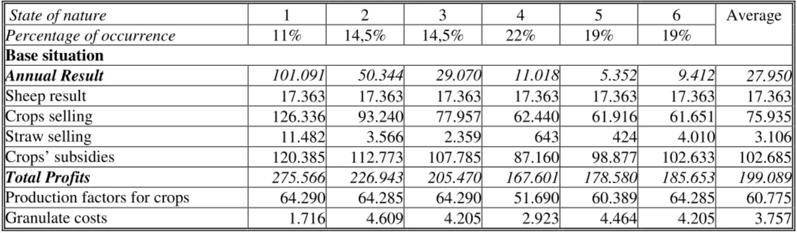
In the next table (table 1) we present the economic model results in what concerns each state of nature annual result, costs and profits for base situation (with only traditional mobilization) and for technological alternatives situation and also the expected values. This annual result should clearly show the farmer’s decision influenced by the different states of nature’s probability of occurrence, and also which is the best exploitation plan for each type of year.
The costs and profits structure is divided as follows:
- Traction costs are in separate lines and divided in fixed costs, variable costs and extra hours’ costs.
- Work costs are also in separated lines, divided in permanent and eventual work. In permanent work we included the sheppard work. Although this is not an integer variable, which means we are talking of sheppard hours, we admit these hours are needed all over the year and so this work should be seen as permanent.
- Profits with products selling and subsidies and costs with other production factors are presented together for all the crops.
- For sheep production we present only the annual result (profits + subsidies – costs with production factors) and, in a separate line, costs with feeding, since animal feeding needs are calculated by the model considering animal needs, feed at disposal from crop activities, selling price for crop products and buying price for sheep granulate.
This way, profits are divided as sheep result, crops selling, straw selling and subsidies to crops and costs are divided as bought production factors for crops, granulate costs, fixed costs, variable costs and extra hours costs with traction, eventual work costs and permanent work costs..
Table 1 – Current results for the studied enterprise and negative deviation, each type of year, expected income and total absolute deviation for base and technological alternatives’ situations. Unit: Euros
State of nature 1 2 3 4 5 6 Average
Percentage of occurrence 11% 14,5% 14,5% 22% 19% 19% Base situation Annual Result 101.091 50.344 29.070 11.018 5.352 9.412 27.950 Sheep result 17.363 17.363 17.363 17.363 17.363 17.363 17.363 Crops selling 126.336 93.240 77.957 62.440 61.916 61.651 75.935 Straw selling 11.482 3.566 2.359 643 424 4.010 3.106 Crops’ subsidies 120.385 112.773 107.785 87.160 98.877 102.633 102.685 Total Profits 275.566 226.943 205.470 167.601 178.580 185.653 199.089
Production factors for crops 64.290 64.285 64.290 51.690 60.389 64.285 60.775
Fixed costs with traction 16.765 16.765 16.765 16.765 16.765 16.765 16.765 Variable costs with traction 64.210 64.180 64.210 51.925 60.749 64.180 60.840
Extra hours costs with traction 0 0 0 6.494 4.270 0 2.240
Eventual work costs 1.766 1.033 1.202 1.057 863 1.082 1.120
Permanent work costs 25.728 25.728 25.728 25.728 25.728 25.728 25.728
Total costs 174.475 176.594 176.400 156.583 173.228 176.240 171.224
Negative deviation each s.n. - - - 16.849 22.521 18.456
Expected income 27.950
Total absolut deviation 57.965
Situação com alternativas tecnológicas Tecnhological alternative situation Annual Result 79.980 160.930 50.940 21.855 18.345 9.805 49.675 Sheep result 16.101 16.101 16.101 16.101 16.101 16.101 16.101 Crops selling 101.520 151.340 79.638 57.881 52.962 48.797 76.727 Straw selling 4.050 10.126 3.876 793 728 4.554 3.654 Crops’ subsidies 115.058 122.046 108.199 89.105 86.107 97.989 100.623 Total Profits 236.729 299.613 207.809 163.875 155.899 167.436 197.103
Production factors for crops 64.624 55.870 65.512 56.648 55.691 65.752 60.246
Granulate costs 5.427 1.521 5.427 5.597 5.597 4.998 4.849
Fixed costs with traction 18.241 18.241 18.241 18.241 18.241 18.241 18.241 Variable costs with traction 42.398 39.071 42.378 35.624 33.958 42.767 38.889 Extra hours costs with traction 7.073 4.240 6.210 7.173 5.292 6.634 6.137
Eventual work costs 1.282 2.225 1.322 888 918 1.362 1.284
Permanent work costs 17.902 17.902 17.902 17.902 17.902 17.902 17.902
Total costs 156.942 139.070 156.992 142.073 137.598 157.655 147.547
Negative deviation each s.n. - - - 27.753 31.260 39.774
Expected income 49.675
Total absolut deviation 99.025
Source: Model results
From this table we can state that in this farm, traditionally a crop farm, the crops are the activities that most contribute to total profits. Subsidies for these activities represented, in the studied year, an important part of this contribution. On the base situation, subsidies contribution for total profits varies, depending on the type of year, between 44 and 55%. On average, this contribution is 51%. On the technological alternatives situation, subsidies contribution for total profits varies between 41 and 59%, being on average 52%.
We can also state that the difference between the two models lies, basically, in traction costs and permanent work costs.
There is an average gain of 29.845 euros from base situation to technological alternatives situation, due to a reduction on variable costs with traction, and permanent work costs, since the farm will need much less traction hours to perform the needed cultural operations. Nevertheless, base situation as an average gain of 5.385 euros when compared to technological alternatives situation, resulting from less fixed costs with traction and less extra hours needed.
The difference on expected income, between the two situations is mainly due to the difference between these values.
So, there is a fundamental costs difference between base and alternative technologies situation. Although the utilization of the machinery the farmer already has leads to lower fixed costs with traction when the traditional technology is used, more days available to work in the field with alternative technologies and a lower necessity of hours to perform cultural operations with these technologies, lead to less tractors need, less permanent workers and less variable costs with traction.
The results presented demonstrate that, although the expected income is positive in both situations, with technological alternatives is 21.725 € higher; in this situation there are 60% of the years, which mean 3 types of years, in which the economic result is lower then expected, but it is never negative. In the base situation the expected income is lower. In this situation the economic result will also be lower then expected in 60% of the years, but it will never be negative.
These results are influenced by three fundamental factors: the production plans, which are
different for the different situations, the available days to work each technology needs and implies and, finally, the farm fixed structure that is a consequence of the first two.
On next tables we present the annual production plans (table 2) and the available days each technology needs and implies (table 3) showing, as we have just stated, that the model considers these aspects and accounts their influence on the economic evaluation of technologies.
TABLE 2–Cultural occupation of soils – rotations and seeded areas (ha) – on base and technological alternatives situations
Type of year 1 2 3 4 5 6
Base situation
Rotations: Sunflower-Durum wheat–Wheat
Clay soils
201,5 201,5 201,5 170,1 201,5 201,5
Rotations: Triticale-Oat-Rest-Rest
Sandy loam soils
185,0 185,0 185,0 123,0 134,9 185,0
Alternative technologies situation
Clay soils Rotations: Sunflower-Durum wheat–Wheat
Sunflower-Barley–Wheat
Direct seeding 57,5 72,8 57,1 51,3 53,2 55,7
Reduced mobilization 144,0 128,6 144,4 112,1 106,4 145,5
Sandy loam soils Rotations: Triticale-Oat–Fallow-Fallow
Direct seeding 185,0 185,0 185,0 185,0 183,6 185,0
Source: Model results
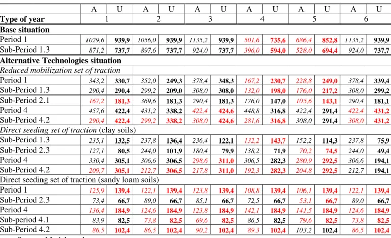
In what concerns the available days each technology has and implies, which decisively influence the model result, as we concluded that the difference between the two situations lies, particularly on costs with traction utilization, we can see in table 3 that, for both situations, the critical periods of traction utilization are different, showing the model considers this aspect in traction utilization for both situations.
Table 3 – Available (A) and used (U) traction hours by critical periods and sub-periods A U A U A U A U A U A U Type of year 1 2 3 4 5 6 Base situation Period 1 1029,6 939,9 1056,0 939,9 1135,2 939,9 501,6 735,6 686,4 852,8 1135,2 939,9 Sub-Period 1.3 871,2 737,7 897,6 737,7 924,0 737,7 396,0 594,0 528,0 694,4 924,0 737,7 Alternative Technologies situation
Reduced mobilization set of traction
Period 1 343,2 330,7 352,0 249,3 378,4 348,3 167,2 230,7 228,8 249,0 378,4 339,4 Sub-Period 1.3 290,4 290,4 299,2 209,0 308,0 308,0 132,0 198,0 176,0 217,2 308,0 299,2 Sub-Period 2.1 167,2 181,3 369,6 181,3 290,4 181,3 176,0 147,0 105,6 143,1 290,4 181,1 Period 4 457,6 422,4 431,2 338,2 422,4 424,6 448,8 316,8 422,4 291,4 422,4 431,2 Sub-Period 4.2 290,4 422,4 299,2 338,2 308,0 424,6 281,6 316,8 308,0 291,4 308,0 431,2
Direct seeding set of traction (clay soils)
Sub-Period 1.3 235,1 132,5 237,8 136,4 236,4 122,1 132,2 143,7 152,2 114,3 237,8 75,9 Sub-Period 2.3 127,1 80,5 244,0 101,9 180,4 79,9 138,2 71,9 70,2 74,5 244,0 49,4 Period 4 330,4 305,1 306,6 306,5 298,6 311,0 306,5 282,3 280,9 292,5 306,6 194,1 Sub-Period 4.2 209,7 305,1 212,7 306,5 217,8 311,0 192,3 282,3 204,8 292,5 212,7 194,1 Direct seeding set of traction (sandy loam soils)
Period 1 125,9 139,4 122,1 139,4 123,8 139,4 108,8 139,4 106,1 139,4 122,1 139,4 Sub-Period 2.3 73,4 66,7 89,0 66,7 85,1 66,7 72,5 66,7 53,1 66,7 89,0 66,7 Period 4 136,4 184,9 124,6 184,9 123,8 184,9 142,1 184,9 141,5 184,9 124,6 184,9 Sub-period 4.1 83,9 82,5 73,8 82,5 69,6 82,5 86,5 82,5 79,6 82,5 73,8 82,5 Sub-Period 4.2 86,5 102,4 86,5 102,4 90,2 102,4 89,3 102,4 103,2 102,4 86,5 102,4
Source: Model results
The most relevant aspects of the cultural occupation of soils presented in table 2 are the fact that alternative soil tillage technologies are always chosen, the non utilization of total clay soils’ area, in year type 4, for both situations, the non utilization of these soils also in year type 5 for the alternative technologies situation and the use of total sandy loam soils’ area in alternative technologies’ situation.
On table 3 we can observe that in base situation the need for traction hours exceeds the availability on period 1 and sub-period 1.3, in states of nature 4 and 5. Since these are winter periods, they have less day light hours and less available days to work in the soil and so the farmer can use only 234 extra hours in period 1 and 198 extra hours in sub-period 1.3. Only in state of nature 4, for both periods, these hours are all used. So these are really the limiting periods and type of year.
For technological alternatives situation the farmer also uses all the extra hours he has during seeding time in state of nature 4. In this type of year, the extra hours are fully used, on reduced
mobilization technology, in period 1.3 (66 hours) and on direct seeding in sandy loam soils in period 1 (30.6 hours). For direct seeding in clay soils this resource never limits the cultural occupation of soils on seeding time.
For state of nature 1, traction resource also limits cultural occupation in sub-period 4.2 for reduced mobilization. In the same sub-period this resource is a limiting resource for states of nature 1, 2, 3, 4 and 5 for direct seeding technology on clay soils. For this technology, but in sandy loam soils, traction is the limiting resource in period 4, for the states of nature 2, 3 and 6.
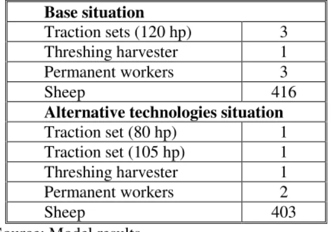
Finally, we shall talk about the fixed structure of the farm, representing long term decisions, and concerning traction sets needed, permanent workers and herd dimension. We can see in table 4 that for the base situation the model chooses 3 traction sets and a threshing harvester, which leads to the need of three permanent workers. For the alternative technologies situation the farmer only needs 2 traction sets, one with a 80 hp tractor for direct seeding and another with a 105 hp tractor for reduced
mobilization and a threshing harvester, which leads to the need of only two permanent workers, although in the average there is more seeded area with these technologies.
In what concerns animals, the feeding resources available maintain 416 heads in the base situation, although these animals are divided in two herds with different nutrition exigencies. One of the herds has 329 animals in a more intensive regimen, selling animals with 3 months and 25 Kg life-weight. The other herd has 87 animals in a more extensive feeding regimen, selling animals with 4 months and 20 Kg life-weight. Their feeding base is composed of triticale and oat straw, pasture from fallows and triticale straw ate in the field. This regimen is complemented with granulated feed when necessary. In less productive years, states of nature 4 and 5, animals also eat oat stubbles. In the technological alternatives situation there is only a herd with 403 animals in the more extensive regimen. Feeding is also based on straw, fallows and granulates when needed.
Table 4 – Traction sets and threshing harvester (n.º), permanent workers (n.º) and herd dimension on the base and alternative technologies situations
Base situation
Traction sets (120 hp) 3 Threshing harvester 1
Permanent workers 3
Sheep 416
Alternative technologies situation Traction set (80 hp) 1 Traction set (105 hp) 1 Threshing harvester 1
Permanent workers 2
Sheep 403
Source: Model results
8. Risk evaluation
A larger expected income on the alternative technologies situation also corresponds to a larger total absolute deviation.
Income risk evaluation for the efficient possible production plans, given the probability
distribution of the defined states of nature allows the definition of a set of admissible plans for the farm that assure the maximum expected income for each level of standard deviation.
With the objective of determining this set we’ve parameterized the restriction that corresponds to the sum of total absolute deviations in 25% steps.
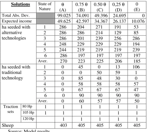
The results, as well as optimal activities levels for each solution, are shown in table 5:
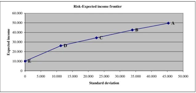
Table 5 – Model results with parameterization of Total Absolute Deviation value – Total Absolute Deviation (€), Expected income (€) and optimal levels of activities
Solutions State of
Nature (A) θ 0.75 θ (B) 0.50 θ (C) 0,25 θ (D) (E) 0
Total Abs. Dev. 99.025 74.091 49.396 24.695 0
Expected income 49.625 42.597 34.367 26.137 10.076 1 286 204 271 191 53 2 286 286 214 129 85 3 286 201 239 256 286 4 248 229 229 229 194 5 244 219 219 219 239 6 286 197 197 197 197 ha seeded with alternative technologies Aver. 270 223 225 206 185 1 0 45 0 13 106 2 0 0 50 59 1 3 0 85 48 30 0 4 0 58 58 58 57 5 0 67 67 67 47 6 0 90 90 90 90 ha seeded with traditional technology Aver. 0 60 57 57 50 80 Hp 1 1 1 1 1 1 105 Hp 1 1 1 1 1 1 Traction sets 120 Hp 1 1 1 1 1 Sheep 403 405 405 405 405
Source: Model results
The frontier that represents the efficient set of production plans, on which the risk is the minimum for each level of expected income, is shown on graphic 1. The letters correspond to those on table 5. On the graphic the income is measured by expected result and risk by its standard deviation, being the variance estimated from the total absolute deviation.
Unit:. Euros
Risk-Expected income frontier
A B C D E 0 10.000 20.000 30.000 40.000 50.000 60.000 0 5.000 10.000 15.000 20.000 25.000 30.000 35.000 40.000 45.000 50.000 Standard deviation E x p ec te d i n co m e
Source: Model results
Graphic 1 – Risk-Expected income frontier
From the farmers point of view, the application of Compromise Programming to the studied economic model, assuming the farmer gives the same weight to both its objectives (obtaining the higher expected income and have the lower variation of this income) has the following results: Table 6 – Studied Model results, for extreme points L1 e L∞ - Total Absolute Deviation and Expected
Income (euros)
Objective function Extreme points
Total Absolute Deviation Expected Income
L1 22.356 25.354
L∞ 43.186 32.297
Source: Model Results
Graphically, these results correspond to the following (graphic 2): Unit. Euros
Risk-Expected income Frontier
L1111 L∞∞∞∞ 0 10.000 20.000 30.000 40.000 50.000 60.000 0 5.000 10.000 15.000 20.000 25.000 30.000 35.000 40.000 45.000 50.000 Standard Deviation E x p ec te d i n co m e
Graphic 2 – Risk-Expected income frontier
According to these results we can state that a farmer who gives the same weights to both its objectives will privilege the utilization of alternative soil tillage technologies but will also use traditional technology. On the average the farmer will mobilize 211 ha of his farm with alternative technologies and only 57 ha with traditional technology.
9. Conclusions
This work proposes a methodology to the soil tillage technology economic evaluation in a risky environment.
The model considers to main aspects:
- The grater income variability resulting from the use of alternative soil tillage
technologies looses importance when compared to the enormous cost difference among the two studied situations – alternative and traditional soil tillage technologies.
- The balance between income risk and the investment - when the farmer is using a set of traction for traditional technology and considers income risk, it is still interesting, from an economic point of view, to continue using traditional technology, which means the farmer’s decision will take this into account. This way, we can think that farmers will let their equipments be fully paid off and only when it will be necessary to
substitute the equipments they will adopt alternative tillage technologies. This result also allows the extrapolation that in a difficult economical situation, that imposes the farmers some investment restrictions, the substitution and adoption of alternative technologies will be even more gradual
We prove the mathematical programming model solution accounts for the probability of occurrence of each state of nature and give an investment solution considering the best production plan for each state of nature.
10. References
Ballestero, E. & Romero, C., 1991 A Theorem Connecting Utility Function Optimization and Compromisse Programming, Operations Research Letters 10 421-427.
Boussard, J-M., 1971 Time Horizon, Objective Function, and Uncertainty in a Multiperiod Model of Firm Growth, American Journal of Agricultural Economics 53 (3) 467-477.
Carvalho, M. L. S., 1994 Efeitos da Variabilidade das Produções Vegetais na Produção Pecuária. Aplicação em Explorações Agro-Pecuárias do Alentejo: Situações Actual e Decorrente da Nova PAC. PhD Thesis Universidade de Évora, Évora.
Cocks, K. D., 1968 Discrete Stochastic Programming, Management Science 85 (1) 73-79. Feder, G., 1980 Farm Size, Risk Aversion and the Adoption of New Technology under Uncertainty, Oxford Economic Papers 32 263-283.
Hardaker, J. B., Huirne, R. B. M. & Anderson, J. R., 1997 Coping with Risk in Agriculture. CAB International, United Kingdom
Hazell, P., 1971 A Linear Alternative to Quadratic and Semivariance Programming for Farm Planning under Uncertainty, American Journal of Agricultural Economics 53 53-62.
Hazell, P. & Norton, R., 1986 Mathematical Programming for Economic Analysis in Agriculture. MacMillan Publishing Company, New York.
Knipscheer, H. C., Menz, K. M. & Verinumbe, I., 1983 The Evaluation of Preliminary Farming Systems Technologies: Zero-Tillage Systems in West Africa, Agricultural Systems 11 95-103.
Kramer, R. et al., 1983 Soil Conservation with Uncertain Revenues and Input Supplies American Journal of Agricultural Economics, 65 694-702.
Marques, C., 1988 Portuguese Entrance into the European Community: Implications for Dryland Agriculture in the Alentejo Region. PhD Thesis, Purdue University, Purdue.
Martins, M. B., 1994 Avaliação Económica de Tecnologias Alternativas de Mobilização do Solo numa Exploração Agrícola Característica da Zona dos Barros de Beja. Master Thesis, Universidade de Évora, Évora.
Rae, A., 1971 Stochastic Programming, Utility, and Sequential Decision Problems in Farm Management American Journal of Agricultural Economics, 53 448-460.
Rae, A., 1994 An Empirical Application and Evaluation of Discrete Stochastic Programming in Farm Management American Journal of Agricultural Economics, 76 625-638.
Romero, C. & Rehman, T., 1985 Goal Programming and Multiple Criteria Decision-Making in Farm Planning: Some Extensions, Journal of Agricultural Economics 39 (2) 171-185. Romero C., Rehman, T. & Domingo, J., 1988 Compromise-Risk Programming for Agricultural Resource Allocation Problems: An Illustration, Journal of Agricultural Economics 39 (2) 271-276.
Romero, C., 1993 Teoria de la Decisión Multicriterio: Conceptos, Técnicas y Aplicaciones. Alianza Universidad Textos, Madrid.
Spharin, I. & Seligman, N. G., 1983 Identification and Selection of Technology for a Specific Agricultural Region: A Case Study of Sheep Husbandry and Dryland Farming in the North Negev of Israel, Agricultural Systems 10 99-125.
Thorton, P. K., 1985 Treatment of Risk in a Crop Protection Information System, Journal of Agricultural Economics,36 (2) 201-209.