P ROJECT E QUITY R ESEARCH – THEV ORTAL CASE

M

ASTER IN

F

INANCE

M

ASTER

’

S

F

INAL

W

ORK

P

ROJECT

E

QUITY

R

ESEARCH

–

THE

V

ORTAL CASE

F

ILIPE

A

MARAL

A

NAHORY

V

ILLARINHO

P

EREIRA

M

ASTER IN

F

INANCE

MASTER’S

FINAL

WORK

PROJECT

EQUITY

RESEARCH

–

THE

VORTAL

CASE

F

ILIPE

A

MARAL

A

NAHORY

V

ILLARINHO

P

EREIRA

O

:

PROF

.

DOUTORA

RAQUEL

MARIA

MEDEIROS

GASPAR

ii

A

BSTRACT

During the course of the last couple of years, some of the largest modern

enterprises have progressed to engage in the public trading environment. The

most notable of these colossal structures are Facebook, Twitter and Alibaba. It

has been debated that companies providing internet services gather some kind of

extra appeal not made explicit by the application of traditional valuation

techniques. So much so that stocks were issued at a value that is much higher

than the base valuation.

Meanwhile, in spite of strong limitations dictated by the weak economic cycle

and financial domestic distress, the Portuguese industry has seen some successful

technological ventures. One of these is an international SaaS provider named

Vortal – the target of our research.

In our study, we value Vortal’s current operations at 34.5 M€ using DCF

methodologies and find its present market price – when compared with others

within the sector – is significantly higher at 41.7 M€. The difference is explained

by considering the value of a call option to expand which reflects the potential

iii

R

ESUMO

Recentemente, algumas das maiores empresas da actualidade prepararam a

colocação das suas acções no mercado. Destas, destacam-se as gigantes Facebook,

Twitter e Alibaba. A propósito destes eventos, discute-se a hipótese de que os

métodos de avaliação tradicionais não captam completamente o valor

reconhecido às empresas que prestam serviços nas tecnologias de informação.

Efectivamente, em alguns casos os preços de subscrição de capital de empresas

nestas condições atingiram valores muito mais altos do que a avaliação inicial.

Entretanto, apesar das limitações impostas por um ciclo económico fraco e uma

conjuntura financeira local adversa, a indústria portuguesa das tecnologias de

informação tem contado com alguns casos de sucesso. Um desses casos é uma

empresa que se dedica à prestação multinacional de serviços de software

chamada Vortal - o objecto do nosso estudo.

No presente estudo, avaliamos a actual operação da Vortal em 34.5 M€ com

recurso à metodologia DCF e determinamos que o seu preço de mercado –

quando comparada com outras empresas do sector – é significativamente

superior, 41.7 M€. A diferença encontrada é explicada através da avaliação de uma opção (de compra) para expandir o negócio que reflecte o crescimento potencial

1

L

IST OF

S

YMBOLS AND

N

OTATIONS

PV– Present Value of the Projected Cash-Flows

n– Number of Periods, Number of Time-Steps

CFi – Cash-Flow at Period i

r– Discount Rate

gS – Sales Growth Rate

gD – Debt Growth Rate

rf – Risk-Free Rate

rm – Market Expected Return

rd – Cost of Debt

Tm – Corporate Income Tax Rate

βu – Unlevered Beta

ru – Unlevered Cost of Equity

re – Cost of Equity

rwacc – Weighted Average Cost of Capital

S0 – Asset Price at Inception

K– Strike Price or Exercise Price

t– Time to Maturity

ɗt– Time-Step Period

σ– Asset Volatility

E[x]– Expected Value Function

f0 – Option Price at Inception

q– Dividend Rate

e– Exponential Operator

N(x) – Cumulative Probability Distribution Function for a Standardized Normal

Distribution

2

L

IST OF

A

BBREVIATIONS

Acc.– Accounts

APV– Adjusted Present Value

B2B– Business-to-Business

B-S– Black & Scholes

CAGR– Compound Annual Growth Rate

CAPEX– Capital Expenditure

CAPM– Capital Asset Pricing Model

CF– Cash-Flow

Cont.– Continuing

CV– Coefficient of Variation

D&A– Depreciation and Amortization

D– Debt

DCF– Discounted Cash-Flow

E– Equity

EBIT– Earnings Before Interest and Taxes

EBITDA– Earnings Before Interest, Taxes, Depreciation and Amortization

EDCF– Enterprise Discounted Cash-Flow

EV– Enterprise Value

FCF– Free Cash-Flow

GDP– Gross Domestic Product

IPO– Initial Public Offering

ISEG– Lisboa School of Economics & Management

IT– Information Technology

ITS– Interest Tax Shield

Liab.– Liabilities

M&A– Mergers and Acquisitions

MFW– Master's Final Work

MM– Modigliani–Miller

NASDAQ– National Association of Securities Dealers Automated Quotations

NOPLAT– Net Operating Profit Less Adjusted Taxes

NYSE– New York Stock Exchange

P&L– Profit and Loss Statement

PERL– Progressive Equity Research

PV– Present Value

R&D– Research and Development

SaaS– Software-as-a-Service

SD– Standard Deviation

SEG– Software Equity Group

SME– Small and Medium Enterprises

UK– United Kingdom

USA– United States of America

3

T

ABLE OF

C

ONTENTS

1. Introduction ... 5

2. Company Overview ... 6

2.1. Financial Position ... 7

2.2. Revenues ... 9

2.3. Earnings ... 11

3. Methodology ... 12

3.1. Discounted Cash-Flow ... 12

3.2. Relative Valuation ... 14

3.3. Contingent Claim Models ... 14

4. Implementation ... 16

4.1. Discounted Cash-Flow ... 16

4.1.1. Financial Statement Rearrangement ... 16

4.1.2. Data Analysis... 16

4.1.3. Income Statement Forecast ... 19

4.1.4. Balance Sheet Forecast ... 20

4.1.5. Cost of Capital ... 22

4.1.6. APV Valuation ... 28

4.1.7. EDCF Valuation ... 31

4.2. Relative Valuation ... 32

4.3. Contingent Claim Models ... 35

4.3.1. A Stochastic Process ... 36

4.3.2. A Binomial Approximation ... 37

4.3.3. A Closed-Form Solution ... 39

4

T

ABLE OF

F

IGURES

Figure 1 - Business Structure [Source: 2013 Vortal Annual Report] ... 7

Figure 2 - Detailed Balance Sheet Proportions ... 8

Figure 3 - Aggregated Balance Sheet Proportions ... 9

Figure 4 - Historical and Forecast Revenues [Source: 2013 Vortal Annual Report] ... 10

Figure 5 - Recent Revenues and Earnings ... 11

Figure 6 - Selected Valuation Methods ...15

Figure 7 - Sales Growth Forecast ... 19

Figure 8 - EV/Revenue Data Collection ... 34

Figure 9 - PERL EV/Revenues v. Recurring Sales Research [Source: PERL, 2013] ... 34

Figure 10 - Stochastic Model Concept ... 36

Figure 11 - Histogram of the APV Stochastic Process ... 37

Figure 12 - Option Pricing from a Binomial Model ... 38

Figure 13 - Option Pricing based on Black-Scholes Formulation ... 40

Figure 14 - Historical Data Sensitivity ... 49

Figure 15 - Cost of Capital, Taxes & Growth Sensitivity ... 50

T

ABLE OF

T

ABLES

Table 2 - Income Statement Forecast ... 20

Table 3 - Balance Sheet Forecast ... 21

Table 4 - Summary of Cost of Capital Projected Rates ... 28

Table 5 - APV Valuation ... 30

Table 6 - EDCF Valuation ... 32

5

1.

I

NTRODUCTION

The purpose of this work is to establish a reasonable value for a business which

provides software services. Vortal operates in several countries and offers specific

applications in a few industries.

Given the nature of this particular business, two complementary approaches to

valuation are considered. Traditional methods based on the calculation of the

present value of future cash-flows form the core of our study but we also

investigate results from the use of real options valuation to compare with the

excess value obtained using comparable multiples from the industry.

The valuation presented herein must be valid from the point of view of any

investor. Otherwise, we would be presenting results lacking the genuineness

found in unbiased market conditions. Therefore, only publicly issued information

by the firm is used to pursuit our aspirations.

This work is supported by the valuation techniques described both by Koller et al.

(2010) and Damodaran (2002). We also take in consideration the works of

Eduardo S. Schwartz and Mark Moon (2000) as well as of Baek, Dupoyet and

Prakash (2008) regarding the stochastic analysis to be implemented.

Furthermore, the approaches to IT and R&D valuation by Serradas (2011) and Tsui

(2005) – respectively – are useful to guide our exploratory exercise. In addition,

we take advantage of geographical and sectorial data listed by Damodaran (2014).

The structure of our work is based on a deductive sequence from the general

analysis to specific implementation and discussion of results. Firstly, we start

with a brief overview of the company in evaluation. Next, we discuss the

methodologies available and applicable to our research. Then, we describe the

implementation of the chosen models with references to the selected data,

6

2.

C

OMPANY

O

VERVIEW

Vortal is a privately owned Portuguese company engaged in providing

e-procurement software services across several countries in Europe as well as in

other parts of the world.

With over 50,000 supplier organizations and over 2,000 buyer corporations using

Vortal at the present time, it’s structure is clearly able to meet the needs of the

largest companies although the focus has been towards mid-market and smaller

businesses.

The company has a headcount of 140 and has developed an international trail

with operations in Portugal, Spain, the Czech Republic and (lately) Colombia.

Clients are predominantly some form of public sector organizations - Vortal has

roughly a 9:1 ratio between public and private/commercial accounts, which

translates approximately into 200 private sector buying organizations using their

solution.

Vortal provides a web platform for professional B2B e-Sourcing and e-Commerce

services, enabling an efficient process through which buyers and suppliers can

connect. The company improves buyer-supplier performance for international

customers in assorted industries including Health, Government, Construction

7

Figure 1 - Business Structure [Source: 2013 Vortal Annual Report]

Recently, Vortal launched eureca.com, a B2B social network with business

transactions as the main driver, supported by a reputation engine to aid

purchasing decisions, replacing unstructured and arduous buying processes such

as email, fax, or phone. Eureca is built on top of a community of agents that drive

business and are rewarded with a share of revenues.

Vortal is the market leader in Spain and Portugal in the Public e-tendering field,

with a market share of 60% and an annual turnover of contracts of about 5,000

million Euros, about 3% of Portuguese GDP and 15% of all public purchases.

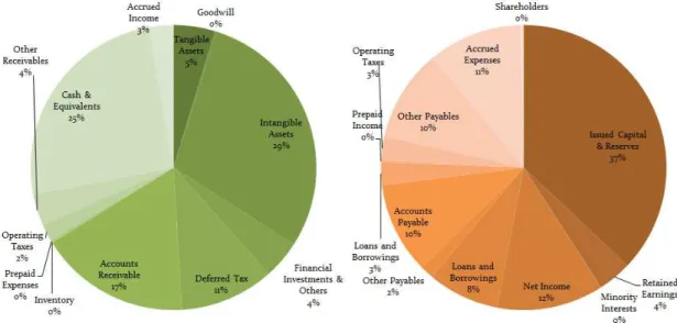
2.1.

F

P

The firm relies on the utilization of intangible assets in form of software

developed in-house as the main resource from which cash-flows are derived.

Vortal maintains a convenient level of cash; typical of a company which is

preparing for investments in the future and does not want be dependent on

8

considered excessive may, in the context of the industry and need for flexibility,

allow for the growth that will meet the potential of the company.

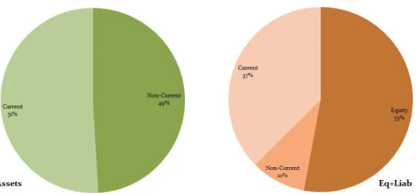
Meanwhile, debt is very diminutive relatively to other sources of financing

operations and equity represents almost 60% of the right side of its balance sheet.

This structure reflects the last 5 years of operation since Vortal engaged in

international campaigns and expanded its market base to include products and

services not customized to a specific industry but rather aiming to reach

additional suppliers and buyers through a more horizontal approach.

9

Figure 3 - Aggregated Balance Sheet Proportions

2.2.

R

Revenue sources in this business may be classified in five major groups from

which Vortal is able to monetize their investments:

 Transaction Fees – charged as a fraction of a certain transaction volume in

a particular operation, mainly directed to the buyer side;

 Subscription Fees – charged on the assumption of anticipated usage and

exposure to the network on an annual basis, more suited to suppliers;

 Advertising – charged for banners, links and logotypes;

 Professional Service Fees – as consultant services to customers at

implementation and training stages;

 Value Added Services Fees – charged for extra services targeted to specific

10

Vortal has been enjoying a healthy rise in revenues since its deployment in 2001

adapting to and taking advantage of several events that mark the history of the

development of the electronic procurement industry in Portugal and abroad.

Figure 4 - Historical and Forecast Revenues [Source: 2013 Vortal Annual Report]

Currently, high expectations are in place for the implementation of the New

European Union Public Procurement Directives which will enforce the use of

technological services and digital platforms for transactions across the continent

in an effort to make the process more transparent and reliable.

Gartner, a highly acclaimed American IT research firm with worldwide

acceptance in the industry, has placed Vortal in the top 5 for e-sourcing and

technology platform and in the top 3 for public sector sourcing. Moreover, in

their latest report “Gartner Magic Quadrant for Strategic Sourcing Suites 2013

Benchmark Report”, Vortal is referred to as having an “exceptional” know-how as

11

Vortal management to feel confident they are able to meet successfully future

challenges either originated externally or from their own development projects.

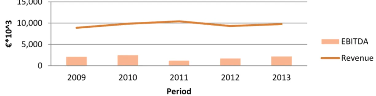
2.3.

E

A slightly erratic earnings profile during the last previous 5 fiscal years shows

nevertheless an interesting maintenance of the level of operating margin which is

not the signature of most of the similar businesses we came across during our

research.

During this period, the company has been able to provide a positive and relevant

net income on a yearly basis. Historically, Vortal has been delivering an

interesting return on investments to its shareholders from which the bulk has

been retained in the firm; dividend policy is subject to shareholders approval for

each financial exercise.

Figure 5 - Recent Revenues and Earnings 0

5,000 10,000 15,000

2009 2010 2011 2012 2013

€

*

10^

3

Period

12

3.

M

ETHODOLOGY

The subjective nature of estimating the value of a certain company allows for a

number of methodologies that may complement one another and provide

different values depending on the objective of the task. Nevertheless, nowadays

most of the authors would agree on four major groups of models which may be

used to accomplish the desired valuation. (Damodaran, 2002)

A comprehensive classification includes:

 Asset Based Valuation – focusing on Liquidation Value or Replacement

Cost of the firm’s Assets;

 Discounted Cash-Flow Models– either dedicated solely to Equity within

the Firm or considering the whole enterprise as the object, and applied to

different growth stages;

 Relative Valuation – based on ratios extracted from comparable

companies for which the value is known;

 Contingent Claim Models – applying real options theory in order to

estimate the worth of a claim on a future payoff attributed to the

difference in value occurring from a change in a particular resource price.

Amongst the above methods, we chose not to include the first one which is more

suitable for companies in distress since it relates to short-term liquidation of the

components of the firm. Moreover, considering the information within reach and

the nature of the business to be valued, we elect the remaining three

methodologies which are detailed ahead in the text.

3.1.

D

C

-F

The concept behind valuation of financial instruments relying on DCF is useful in

13

for future inflows generated by selected assets through a predefined period of

time (which may be extended until perpetuity) and calculate the sum of the

present value of each cash-flow employing a suitable discount rate which allows

for the time-value concession within our results. In general,

(1) 𝑃𝑉 = ∑ 𝐶𝐹𝑖

(1 + 𝑟)𝑖 𝑛

𝑖=1

The selection of the discount rate to use in our present value calculations is not

trivial and depends on the information available. This discount rate may be

interpreted as the opportunity cost the investor bears while having his resources

allocated to that particular project or firm. We may also refer to this discount rate

as a return on the capital employed to generate the desired cash-flows.

Since we are focusing our valuation on the information released by the company

in the form of its annual reports for the last 5 fiscal years, we need to compute an

appropriate discount rate referring to the obtainable data.

Consequently, we prefer the model which simultaneously allows us to employ the

simplest discount rate that we can estimate as well as to build a cash-flow

sequence that may be predicted taking into account the recent performance of

the firm and conventional assumptions for the future. This model is referred to as

the Adjusted Present Value (APV) method and consists of the use of DCF to a

virtually unlevered firm adding eventually the fiscal benefits resulting from the

incurred debt to finance operations.

As a means to support the APV valuation we also calculate the present value

based on the Enterprise Discounted Cash-Flow (EDCF) approach which relies on

the Weighted Average Cost of Capital (WACC) and the assumption of a

predetermined target for the capital structure to finance the operations that may

not be a good conjecture in our case. Nevertheless, and since we depend on the

industry statistics in either case, we expect to reach values that should lead to

14

Both models are built in two parts regarding the time frame of our forecasts for

the future cash-flows. The first three years of forecasted operations are

designated by the explicit period and the fourth year represents a repeating

pattern for the perpetuity (Terminal Value) which we refer to as the continuing

period.

3.2.

R

V

Regarding the means to compare our firm to others in the industry in order to

search for a value which replicates the current conditions in the market, the

approach recommended is the Relative Valuation.

Assuming we are able to find similar companies for which we may successfully

investigate a certain number of valuation ratios applicable to the firm in study,

we would then be able to estimate the worth of our firm by multiplying those

ratios by the appropriate measure found in the company’s records. Usually

referred to as Multiples, these ratios are references for the price of an asset (or a

set of assets that jointly compose a company) that should point towards the

current context within the stock markets or the M&A activity.

Although simple in its formulation, this method requires a sound process of

selecting the so-called similar companies and a certain degree of good chance

that for those few truly comparable firms that are chosen there is enough

information available at the relevant time.

Finding similar businesses with accessible data is challenging because no two

enterprises are alike and only publicly traded firms have the obligation to provide

financial details and a credible market value.

3.3.

C

C

M

In the event of obtaining results - generated from the above mentioned

15

explained otherwise, we establish a rationalization for that difference in value by

referring to some theoretical justifications which recommend the use of real

options methods to value some part of the company’s assets that may not be fully

integrated in the previous calculations.

In this context, a contingent claim may be interpreted as an option contained

within the special characteristics of a firm which would allow its owners,

sometime in the future, to capitalize on a particularly favorable turn of events

that would increase the value of the original project, investment or operation.

The described prospect has in itself a quantifiable value and may be the cause for

certain discrepancies recorded recently in stock markets.

In our study we apply two different approaches in order to try to establish an

eventual discrepancy exposed by the results obtained from the traditional

methods.

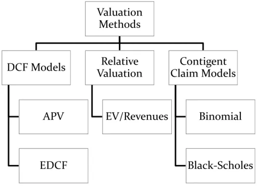
Figure 6 - Selected Valuation Methods

Valuation

Methods

DCF Models

APV

EDCF

Relative

Valuation

EV/Revenues

Contigent

Claim Models

Binomial

16

4.

I

MPLEMENTATION

4.1.

D

C

-F

4.1.1.FINANCIAL STATEMENT REARRANGEMENT

We select the last five years (ending in 2103) of financial information issued by

Vortal because they represent the most recent stable characteristics of the firm in

its newest setup as an internationalized group of subsidiaries. Appendix 1 and

Appendix 2 summarize all the historical data collected.

By rearranging the above mentioned information, we are able to proceed on our

analysis independently of the accounting principles followed by the firm besides

allowing us to identify other major traits of the operation such as: CAPEX, Debt

and Working Capital; Risk Assessment and Capital Structure; Efficiency and

Performance. Appendix 3 and Appendix 4 show the result of this procedure.

4.1.2.DATA ANALYSIS

The rearrangement of the firm’s information together with the analysis of

patterns and trends for the major items in the financial statements allows us to

organize a forecast for the future operations of Vortal.

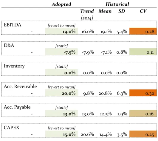
FORECASTING RATIOS AND STATISTICS

For the appropriate lines in the financial statements, we study the historical

patterns and trends in order to choose the suitable ratios which allow us to

project the operations into the future. These ratios refer to Sales and are

summarized in the next table.

In general, we opt to attribute a reversion to the mean as the expected value to

consider in our forecast. Elsewhere, we consider the parameter to be static over

17

Adopted Historical

Trend Mean SD CV

[2014]

EBITDA [revert to mean]

- 19.0% 16.0% 19.1% 5.4% 0.28

D&A [static]

- -7.5% -7.9% -7.1% 0.8% 0.11

Inventory [static]

- 0.0% 0.0% 0.0% 0.0%

Acc. Receivable [revert to mean]

- 20.0% 9.8% 20.8% 6.3% 0.30

Acc. Payable [static]

- 13.0% 13.0% 12.5% 1.9% 0.16

CAPEX [revert to mean]

- 15.0% 20.6% 14.4% 3.5% 0.25

Table 1 - To-Sales Ratio Analysis and Selection

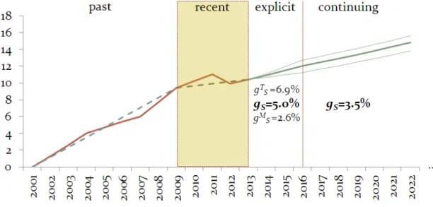
GROWTH PROJECTIONS

Revenues show an upward trend with a compound annual growth rate (CAGR) of

2.7%. The statistics display a somewhat intermittent behavior during recent years

– reflected in a standard deviation of 8.8% on the year-over-year relative change

with a mean of 2.6% – mainly influenced by an uncharacteristic year of 2012 when

the effects of the domestic economic distress originated the first downward move

in a steadily expanding history of Vortal’s sales.

Adjusting our measurements by removing the above mentioned outlier we obtain

different and considerably more accurate figures: an average annual revenue

growth rate of 6.9% accompanied by a 1.9% standard deviation.

Given our conservative goal on the implementation of the chosen DCF

18

that may occur again in the next few years in the domestic market, we opt to use

the last year change rate of 5% to extend through the explicit period of our

forecast.

As for the perpetual component (continuing period) of our prediction, we take in

consideration macroeconomic outlooks for the countries and industries the firm

is serving and establish a compatible revenue growth rate.

Considering the dependency of the firm’s revenues on the investment in

infrastructure that impact both on the public procurement and private activities

for which the services of Vortal are vital, we refer to a report published by the

McKinsey Global Institute which suggests that growth in infrastructure

investment must, at least, be the same as GDP’s in the long-term future. (Dobbs

et al., 2013)

It is incontestable that, in the long-term, one of the most certain policies to be

adopted by the majority of the central banks is to maintain a controlled level of

inflation in the surroundings of a 2% annual rate. Hence, the growth of revenues

obtained from our company in a model based in current prices (in the long term)

shall be at least the expected level of inflation.

Moreover, the outlook medium-term projections for the global economy

(International Monetary Fund, 2013), suggests for the period between 2015 and

2018 a World Real GDP Growth in the Euro Area of 1.6%. This figure, for

usefulness, is adjusted for inflation - since our estimates are calculated in current

prices. Hence, our best estimate based on the above mentioned data would be a

nominal terminal growth rate of (1.02 × 1.016 − 1 =)3.63%; capturing the

combined effect to simulate current prices.

Nevertheless, in a conservative approach, we must focus on the fact that in the

Portuguese market lays the majority of Vortal’s influence and historically the

domestic growth trials behind the rest of the world advanced economies.

19

a proxy for our long-term projections. Hence, we settle for a more modest growth

rate of 3.5% reflecting the current circumstances.

Figure 7 - Sales Growth Forecast

The above graph highlights the chosen path and discussed boundaries.

4.1.3.INCOME STATEMENT FORECAST

Expenses due to interest bearing debt have a regular pattern in the books of

Vortal. They account to a little more than 6% of the previous year long-term

borrowing responsibilities of the firm. At this stage we could implement the

mentioned rate in our model but this is not the best practice. The theoretically

expected Cost of Debt (detailed ahead in this document) is recommended and we

adopt the rate of 5.4% instead.

Taxes payable annually to the Government of Portugal are based on the

geographical rates that must apply to a local surcharge increased by a state

surtax; identified as “derramas”. The resulting rate amounts to 27.5%. (PricewaterhouseCoopers Portugal, 2014)

Both Interest Income and Minority Interests, due to their irrelevancy, are

20

€*10^3

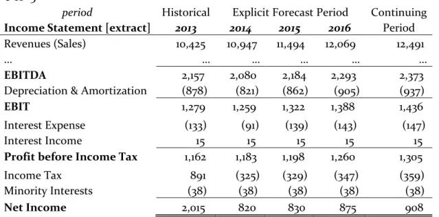
period Historical Explicit Forecast Period Continuing

Income Statement [extract] 2013 2014 2015 2016 Period

Revenues (Sales) 10,425 10,947 11,494 12,069 12,491

… … … … … …

EBITDA 2,157 2,080 2,184 2,293 2,373

Depreciation & Amortization (878) (821) (862) (905) (937)

EBIT 1,279 1,259 1,322 1,388 1,436

Interest Expense (133) (91) (139) (143) (147) Interest Income 15 15 15 15 15 Profit before Income Tax 1,162 1,183 1,198 1,260 1,305 Income Tax 891 (325) (329) (347) (359) Minority Interests (38) (38) (38) (38) (38) Net Income 2,015 820 830 875 908

Table 2 - Income Statement Forecast

4.1.4. BALANCE SHEET FORECAST

Intangible Assets account, as mentioned before, is the core of the business in our

study. Computation of the future exercises’ relevant figures in this account his

accomplished by taking the previous year record and adding (the negative value)

of the current year Depreciation & Amortization line from the Income Statement

plus the homologous Capital Expenditure value.

Remaining Assets – including Cash & Equivalents and Tangibles – are assumed to

remain constant and equal to the latest annual record; 2013.

Estimation of Shareholders’ Equity results from the previous year amount added to the same year Net Income; as a measure of Retained Earnings.

Remaining Liabilities – and Minority Interests but not Total Debt – are constant

and equal to the latest annual record; 2013.

We refer at this point to the elementary balance sheet equation:

21

In order to obtain the outstanding Total Debt account we apply equation (2) and

iterative calculations. In this way, we are able to project Total Debt through the

years as result of all previously mentioned results.

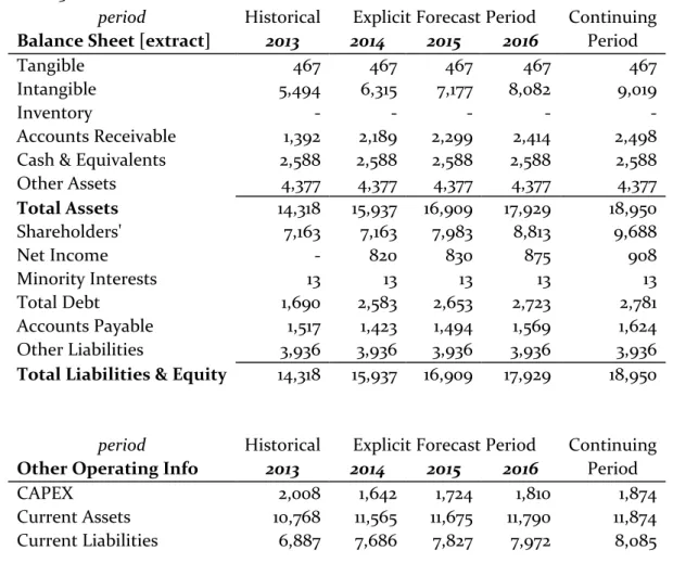
€*10^3

period Historical Explicit Forecast Period Continuing

Balance Sheet [extract] 2013 2014 2015 2016 Period

Tangible 467 467 467 467 467 Intangible 5,494 6,315 7,177 8,082 9,019 Inventory - - - - - Accounts Receivable 1,392 2,189 2,299 2,414 2,498 Cash & Equivalents 2,588 2,588 2,588 2,588 2,588 Other Assets 4,377 4,377 4,377 4,377 4,377 Total Assets 14,318 15,937 16,909 17,929 18,950 Shareholders' 7,163 7,163 7,983 8,813 9,688 Net Income - 820 830 875 908 Minority Interests 13 13 13 13 13 Total Debt 1,690 2,583 2,653 2,723 2,781 Accounts Payable 1,517 1,423 1,494 1,569 1,624 Other Liabilities 3,936 3,936 3,936 3,936 3,936 Total Liabilities & Equity 14,318 15,937 16,909 17,929 18,950

period Historical Explicit Forecast Period Continuing

Other Operating Info 2013 2014 2015 2016 Period

CAPEX 2,008 1,642 1,724 1,810 1,874 Current Assets 10,768 11,565 11,675 11,790 11,874 Current Liabilities 6,887 7,686 7,827 7,972 8,085

Table 3 - Balance Sheet Forecast

It is important to note that we traced during this analysis a slightly degrading

trend in the Working Capital of the firm which has been consistently decreasing

throughout the last 5 years culminating with a negative figure during the year of

2013 exercise. It is an outcome of the decaying efficiency registered in the recent

past due to increasingly extended periods of collection from customers.

We associate this condition to the recent reducing management ability to

22

historical analysis. On the other hand, Vortal is poised to operate on a

multinational frame in a more consolidated fashion and will take advantage of

operating in more balanced foreign economies. Therefore, and without

compromising the goals of our overall assessments, we assume a stabilization of

operating conditions in our future projections of Working Capital reverting to the

mean at a manageable level.

4.1.5.COST OF CAPITAL

As mentioned previously, the cost of capital includes a crucial set of parameters

in the exercise of the DCF methodology. It represents the time-value of money

and appears in the form of annualized rates which affect the computation of the

desired Present Values, discounting the above revealed projected cash-flows.

In our study, we require two different (although interrelated) rates to implement

in the different models: APV and EDCF. These are the Unlevered Cost of Equity

and the Weighted Average Cost of Capital, respectively.

RISK-FREE RATE

A measure of the opportunity cost, prevailing in the market, for which there is a

zero probability of default embodies the reference and the basis of all the

methodologies applied herein.

Presently, the concept of the availability of an investment instrument exempt of

the possibility of failing to see its capital entirely refunded at maturity is a rather

theoretical one – given the prospect of default even by the most solid of states

issuing debt. The recent global financial crisis as presented us with some palpable

examples of sovereign responsibilities in the brink of not being met or requiring

transnational support in order to be honored – namely in the European countries

23

Nevertheless, some of the reviewed literature offer guidelines in choosing the

appropriate vehicle of investment for the model and timing being developed.

(Damodaran, 2002) (Koller et al., 2010)

Thus, we chose a government bond: with the higher possible degree of

credibility, issued in the currency with which the firm reports its taxes and

trading with sufficient liquidity to simulate the risk-free environment we want to

model.

The above mentioned financial instrument, given the required traits and market

constraints, is the 10-year German Bund. Currently trading at an annual rate of

1.17%, which is the figure we adopt. (Bloomberg, n.d.)

MARKET RISK PREMIUM

A local historical statistic of the difference between the expected return on a

market portfolio and the risk-free rate, on a yearly basis, is used as the projection

of an important component of the postulate commonly referred to as Capital

Asset Pricing Model. This hypothesis, CAPM, establishes a relationship between

risk and expected return on an individual asset by accommodating a risk measure

named beta (β) and providing anticipated results for the return on the security

we are investigating. (Koller et al., 2010)

It is equated as follows:

(3) 𝑟_𝑖 = 𝑟_𝑓+ 𝛽_𝑖(𝑟_𝑀− 𝑟_𝑓)

Where,

ri is the expected return on the chosen security, and

βi is the beta as a measure of risk of the chosen security

For the purpose of our study, this formulation is very useful to derive other

24

Relying on the research available from the records updated at the New York

University Stern School of Business, we look for the value listed for our country of

reference – Germany – and adopt an annual rate of 5%. (Damodaran, 2014)

COST OF DEBT

As mentioned earlier in the document this cost may be estimated, although in

many instances returning weak results, by collecting historical data from the

company. Vortal has not issued any debt in the past and it is not expected to do

so in the future. The company’s means of financing of its operations, apart from

the excess cash collected through the years and subscribed equity in its

foundation, is by borrowing from commercial banks a small fraction of its

necessities.

The recommended alternative is by means of the Synthetic Ratings Approach

adjusted to the domestic reality as a function of the relevant country default risk.

(Damodaran, 2002)

In the present case, the country to which we must refer to regarding borrowing

costs to be supported by Vortal is Portugal. Currently the Portuguese crisis,

originated by difficulties in meeting responsibilities attached to issued sovereign

debt, has driven the fear of default to unimaginable heights. Hence, the present

rating associated with the country - which has had a systemic impact on the

financial activities of all the economic agents – must be taken into consideration

when evaluating the costs related to debt contracted by Portuguese companies.

So, our implementation of the Synthetic Ratings Approach – adjusting for a

country with unusually high Default Risk premium – assigns the theoretical Cost

of Debt for Vortal as follows:

(4) _{𝑟𝑓+ 𝐶𝑜𝑚𝑝𝑎𝑛𝑦 𝐷𝑒𝑓𝑎𝑢𝑙𝑡 𝑆𝑝𝑟𝑒𝑎𝑑 +}2

25

Again, trusting the research accessible from the records updated at the Stern

School of Business, we look for the listed country of fiscal reporting of Vortal

(Portugal) and adopt a Country Default Spread of 5.36%. (Damodaran, 2014)

We are in a position to obtain the Company Default Spread based on the latest

Interest Cover Ratio obtained from the analysis of historical operations of Vortal.

Making use of the data collected in the above mentioned records of NYU Stern,

we verify that for a figure of 9.6 during the year of 2013 we are lead towards a

Aa2/AA rating and a spread of 0.7%. (Damodaran, 2014)

The use of equation (4) with the extracted values results in an estimated Cost of

Debt for the firm of 5.4%.

UNLEVERED BETA,UNLEVERED COST OF EQUITY

In order to proceed with the implementation of the APV model we need an

estimation of the cost of capital the firm would support if no debt is present to

use as the appropriate discount rate.

The Unlevered Cost of Equity may be obtained using the following formulation:

(5) 𝑟_𝑢 = 𝑟_𝑓+ 𝛽_𝑢(𝑟_𝑀− 𝑟_𝑓)

This last parameter - Unlevered Beta – ideally, considering that it represents the

risk associated with the assets of the firm independently of the financial structure

supporting the operations, should be a characteristic of the industry where the

company operates. Since the assets and the business are the same for a selected

group of companies offering the same services, there should be a common

measure of risk separating the mentioned group from the others in the market.

It is understood that in order to compute the desired Unlevered Cost of Equity

we may take advantage of aggregated data organized by industry to extract the

26

Currently, in the case of the Internet Software and Services industry, Unlevered

Beta levels at 1.01 – thus, a fraction riskier than the market.

Consequently, the adopted value for the Unlevered Cost of Equity is 6.2%.

This concludes the necessary set of inputs to successfully implement the

Adjusted Present Value model.

TARGET LEVERAGE RATIO

The alternative approach to the Adjusted Present Value model is the Enterprise

Discounted Cash-Flow model. This formulation, although deemed to return a

similar valuation to the APV as a consequence of Modigliani-Miller theorems

(Koller et al., 2010), is of interest for us as a means of validation and calibration of

our study. Nevertheless, the caveat of following the EDCF path lies on the

imposition of a target leverage ratio for the firm during projected years.

In order to establish such requirement we must refer to industry statistics which

allows us to define a legitimate capital structure for the business in analysis.

Hence, we begin by selecting from the already mentioned NYU Stern Industry

references the appropriate D/E ratio of 4.16%. (Damodaran, 2014)

This assumption contrasts with the historical and forecasted patterns where we

are able to verify a considerably different proportion in the financing capital of

Vortal’s business. In fact, although the trend shows a path to a positive leverage ratio, the current position regarding the firm’s excess cash turns the sign of the mentioned ratio to negative - a consequence of a systematic negative Net Debt

value.

Nonetheless, for the purpose of the present exercise there is no incongruence in

27

COST OF EQUITY

As a consequence of our assumption of the firm’s capital structure for the future,

together with results from the Cost of Debt assessment and Unlevered Cost of

Equity investigation, we may now use a combination of the Capital Asset Pricing

Model theory and Modigliani and Miller’s equations to estimate Cost of Equity.

(Koller et al., 2010)

(6) _{𝑟𝑒 = 𝑟𝑢+}𝐷

𝐸(𝑟𝑢− 𝑟𝑑)

The ensuing result is the adoption of an annual rate of 6.25% for this particular

parameter.

WEIGHTED AVERAGE COST OF CAPITAL

Distinctively to the APV computation, the EDCF approach calls for a discount

rate based on the WACC formulation in order to capture the capital structure

discussed above:

(7) _{𝑟𝑤𝑎𝑐𝑐 =} 𝐷

𝐷 + 𝐸 𝑟𝑑(1 − 𝑇𝑚) + 𝐸 𝐷 + 𝐸 𝑟𝑒

The result of the above calculation is a WACC annual rate of 6.16%.

This shows a very similar rate to the Cost of Equity computed before and is a

consequence of the extremely low leverage ratio in the industry reflected in our

28

Adopted Lower Upper Reference Comment

Limit Limit

Risk-Free rf 1.17% 1.17% 10-year Yield Ger. _Bund

Market Premium rm-rf 5.0% 4.5% 5.5% 5.00% Damodaran 2014

Cost of Debt rd 5.4% 5.4% 6.0% 5.36% add 2/3 country risk [estimated] [historical]

Unlevered Beta βu 101.0%

101.00% Damodaran 2014

Unlevered Cost ru 6.2% [APV]

WACC rwacc 6.16% [EDCF]

Table 4 - Summary of Cost of Capital Projected Rates

4.1.6. APVVALUATION

Our deterministic approach to the value of the firm begins by establishing a

reasonable forecast for the Net Operating Profit Less Adjusted Taxes (NOPLAT)

as a starting point for the Free Cash Flow available to all investors. We then

compute the Present Value of the Enterprise as if the Company was All-Equity

Financed – considering our estimate for the Unlevered Cost of Equity – and,

finally, we add to the result the Present Value of Tax Shield benefits generated by

debt contracted through the years. (Koller et al., 2010)

Free Cash Flow forecasted for next three years (on an explicit basis) and for the

fourth year (to simulate a continuing condition) are calculated. Taking in

consideration the fact that we are using historical data of the company’s last five

annual exercises our explicit forecast must not extend beyond the time frame of

29

seeking to predict, we use an adjusted version of NOPLAT (or after-tax EBIT) as

well as the necessary deductions of Net Investments from the result.

The chronological change in the Operating Working Capital is instrumental to

achieve the overall deductions of the above mentioned Net Investments. It is

obtained from our forecasted Balance Sheets.

Note the particularity, in the context of the continuing forecasted period to

achieve what is usually referred to as Terminal Value, of omitting the

contribution of D&A and CAPEX to the computation of Free Cash-Flow as it is

presumed that in perpetuity these two accounts cancel each other out.

Interest Expenses throughout the years of projection is computed in order to

establish the Interest Tax Shield – the annual savings deducted from the Net

Income to be added in adjustment of our discounted cash-flow sums. These

expenses are calculated as a fraction of Total Debt running in the previous year at

the estimated rate for the Cost of Debt clarified above.

The present value of FCF from Operations has two components. One given by the

sum of discounted cash-flows computed by using equation (1), the other given by

the Gordon Growth Model resulting in the Terminal Value. (Damodaran, 2002)

(8) _{𝑃𝑉𝐶𝐹 = ∑} 𝐶𝐹𝑖

(1 + 𝑟𝑢)𝑖+ 3

𝑖=1

[𝐶𝐹4⁄(𝑟𝑢− 𝑔𝑆𝑐𝑜𝑛𝑡𝑖𝑛𝑢𝑖𝑛𝑔)] (1 + 𝑟𝑢)3

Analogously, the Present value of Interest Tax Shields is computed in two steps.

(9) 𝑃𝑉_𝐼𝑇𝑆 = ∑ 𝐼𝑇𝑆𝑖

(1 + 𝑟𝑑)𝑖 + 3

𝑖=1

[𝐼𝑇𝑆4⁄(𝑟𝑑− 𝑔𝐷)] (1 + 𝑟𝑑)3

Total Debt Growth Rate, gD, for the continuing period is assumed to be equal to

the growth value obtained directly from the building of our Forecasted Balance

Sheet – in this instance, accordingly, both values are a result of our previous

30

Moreover, we are hence able to compute our estimate for the Adjusted Present

Value as follows. (Koller et al., 2010)

(10) 𝐴𝑃𝑉 = 𝑃𝑉_𝐶𝐹+ 𝑃𝑉_𝐼𝑇𝑆

Since the described model returns a valuation of the operations of the firm, in

other words the economic benefit obtained from the use of the operating assets

against the loss incurred from the use of the operating liabilities, we add Cash

and other Assets and deduct other Liabilities accounts to the Adjusted Present

Value in order to obtain the desired Enterprise Value.

€*10^3

period Cont.

Cash Flows 31-12-2012 31-12-2013 2014 2015 2016 2017

EBIT x (1-Tm) NOPLAT 928 913 958 1,006 1,041 Depreciation and Amortization 878 821 862 905

Change in Operating Working Capital (879) 892 38 40 30

CAPEX 2,008 1,642 1,724 1,810

Free Cash-Flow 676 (800) 58 61 1,012

Inventory - - - -

-Acc. Receivable 1,688 1,392 2,189 2,299 2,414 2,498

Acc. Payable 935 1,517 1,423 1,494 1,569 1,624

Operating Net Working Capital 754 (125) 766 805 845 874

Change in Operating Working Capital (879) 892 38 40 30

Interest Expense (91) (139) (143) (147)

Interest Tax Shield 25 38 39 40

period 0 1 2 3 4

Present value of FCF from Operations Explicit (651) (753) 51 51

Terminal Value from Operations Cont. 31,041 844

Present value of Interest Tax Shields Explicit 92 24 35 34

Terminal Value of ITS Cont. 953 35

Cash & Equivalents 2,588

Other Assets 4,377

Other Liabilities (3,936)

Enterprise Value 34,464

Explicit Historical

31

4.1.7.EDCFVALUATION

EDCF follows the same principles applied in the APV approach.

This approach is also based in the above mentioned Net Operating Profit Less

Adjusted Taxes (NOPLAT) as a starting point for the Free Cash Flow available to

all investors. Nevertheless, the Present Value of the Enterprise is obtained

considering, in this instance, our estimate for the WACC alone. (Koller et al.,

2010)

Free Cash Flows are calculated in the same way for the relevant periods taking

advantage of an adjusted version of NOPLAT (or after-tax EBIT) as well as the

necessary deductions of Net Investments from the result.

The present value of FCF from Operations has again two components. One given

by the sum of discounted cash/flows computed by using equation (1), the other

given by the Gordon Growth Model resulting in the Terminal Value. This

approach requires a different discount rate, as explained, which is an average

allowing for the adopted capital structure – the weighted average cost of capital.

(Damodaran, 2002)

(11) _{𝑃𝑉𝐶𝐹 = ∑} 𝐶𝐹𝑖

(1 + 𝑟𝑤𝑎𝑐𝑐)𝑖+ 3

𝑖=1

[𝐶𝐹4⁄(𝑟𝑤𝑎𝑐𝑐− 𝑔𝑆𝑐𝑜𝑛𝑡𝑖𝑛𝑢𝑖𝑛𝑔)] (1 + 𝑟𝑤𝑎𝑐𝑐)3

Our estimate for the Enterprise Discounted Cash-Flow is subsequently the

resulting value for PVCF which is added to the current value in Cash &

Equivalents, Other Assets and Other Liabilities accounts to project the desired

32

€*10^3

period Cont.

Cash Flows 31-12-2012 31-12-2013 2014 2015 2016 2017

EBIT x (1-Tm) NOPLAT 928 913 958 1,006 1,041 Depreciation and Amortization 878 821 862 905

Change in Operating Working Capital (879) 892 38 40 30

CAPEX 2,008 1,642 1,724 1,810

Free Cash-Flow 676 (800) 58 61 1,012

Inventory - - - -

-Acc. Receivable 1,688 1,392 2,189 2,299 2,414 2,498

Acc. Payable 935 1,517 1,423 1,494 1,569 1,624

Operating Net Working Capital 754 (125) 766 805 845 874

Change in Operating Working Capital (879) 892 38 40 30

period 0 1 2 3 4

Present value of FCF from Operations Explicit (651) (753) 51 51

Terminal Value from Operations Cont. 31,786 846

Cash & Equivalents 2,588

Other Assets 4,377

Other Liabilities (3,936)

Enterprise Value 34,165

Historical Explicit

Table 6 - EDCF Valuation

As expected, and already discussed herein, similar results are obtained by the use

of the two methods.

4.2.

R

V

Relative valuation requires a certain degree of criteria and available information.

Although this approach is in practice the preferred and the most utilized

although rather subjective, in order to successfully perform the desired valuation

the analyst must chose comparable firms carefully and enjoy the chance of being

able to compile enough information to support his choices. (Damodaran, 2002)

Recently, there have been a few acquisitions (Ariba, SciQuest and

CombineNet) from which we are capable of gathering sufficient data to employ

33

Moreover, we are able to identify - through the already mentioned report on the

top e-sourcing firms where Vortal has been included – a couple of competitors

currently trading in the US stock exchange from which it is possible to register

relevant data. (Gartner, 2013)

Furthermore, we rely on aggregated sectorial data compiled by two firms

dedicated to the United States and European markets and particularly the

industry sector in which Vortal operates; SEG and PERL respectively. (Software

Equity Group, L.L.C., 2014) (Progressive Equity Research Limited, 2013)

Ideally we should consider at least three different multiples to include in our

work: one user-based and two related to the Enterprise Value, either referred to

Revenues or EBITDA.

We are unable to use the suggested user-based approach (Cauwels & Sornette,

2011) due to the lack of information regarding most of the analyzed firms.

Also, and given the highly erratic nature of all of the businesses’ earnings

historical values, we are forced to leave the EBITDA multiple behind limiting our

study to the Revenue side of our comparison.

The above mentioned limitations reinforced our focus on compiling as much

valid information as possible regarding the selected EV/Revenues multiple.

Considering the recent acquisitions of Ariba by SAP and current stock prices of

SciQuest and CombineNet, we would be inclined to adopt a figure in the

neighborhood of 6 times Revenues achieved in the latest exercise.

On the other hand, the results reported by SEG from companies of similar levels

of Revenue Growth, aim toward a lower multiple of 2.5 times Revenues.

A summary of the collected data is illustrated in the following diagram, showing

34

Figure 8 - EV/Revenue Data Collection

35

Based on Vortal’s last annual report we estimate that recurring revenues add up

to approximately 73% of revenues realized by Vortal during the year 2013; mainly

from Suppliers wishing to engage in Vortal’s network and Corporate Buyers who

take advantage of its services on a regular basis. By taking this value in Figure 9

and crossing the line produced by the PERL team we are able to identify a

conservative value of 4 which we consider to be the market valuation at this stage

for a company like Vortal.

Thus, the market value of Vortal is the last reported figure regarding Revenues

(or Sales) which is 10,425 €*10^3 times 4 resulting in a valuation of 41,701 €*10^3.

41.701 M€ = 4x 10.425M€

4.3.

C

C

M

If we agree that the market value of Vortal is given by our Relative Valuation of

the company and that the DCF approach is not able to materialize all of the value

of a company of this type – as a corollary of the arguments and results we

describe in the first chapters of this work – we must also consent with the

necessity to identify another source of value to fill in the gap.

We understand now that value is driven by revenues (and maybe also by the

number of active users) and eventually the stableness implied by the DCF

approach does not accommodate or project dramatic rises in sales as well as

spectacular decreases in that particular side of the business.

The valuation of modern companies like Vortal with the help of non-traditional

methods that try to go beyond is well documented and a few successful examples

emerge. One of those cases addresses the problem of projecting R&D investments

into the future within large scale enterprises and constitutes a comprehensive

analysis of the empirical evidence. (Tsui, 2005) Another model, in 2000 and

36

which has rendered acceptable results in the explanation of higher than expected

market values for a few IT companies. (Schwartz & Moon, 2000) (Baek et al.,

2008)

4.3.1.ASTOCHASTIC PROCESS

Influenced by these novel approaches, we adapt our spreadsheets - created to

obtain the DCF valuation - and perform simulations in order to achieve the

necessary results leading to the implementation of real option pricing models.

In our work, we develop a means to obtain a measure of the desired volatility by

simulating several results from our selected deterministic valuation model (APV)

through the conversion of one of the most sensitive parameters in a

randomly-based variable – Revenue Growth. (Refer to Appendix 5: Sensitivity Analysis)

From the historical data we assume a normal distribution with known mean and

standard deviation – in our exercise: 2.6% and 8.8% respectively. Then, we

substitute the deterministic baseline value by a function that generates the

desired random figures based on the mentioned distribution.

37

The number of trials chosen (3,000) imparts, considering a 95% confidence

interval, an acceptable error in our estimation of the Enterprise Value which has

a value of approximately ±0.3 M€ given the standard deviation of around 7.6 M€;

expressed by the formula:

±1.96 ×_√3,0007.6𝑀€

The outcome of this procedure is patent in the following graph and consistently

returns a Coefficient of Variation of 23%.

Figure 11 - Histogram of the APV Stochastic Process

4.3.2. ABINOMIAL APPROXIMATION

The possibility of finding in Vortal’s operation and assets the option to expand is tested by idealizing a consistent frame of problem formulation in the context of

38

For this purpose we take advantage of a simplistic but attractive approach which

obtains an estimate of the desired valuation by means of the proven

methodologies used in the financial option pricing techniques. (Serradas, 2011)

We perceive the origin of the extra value we are assessing as a call option

susceptible of being exercised during the lifetime of a common R&D project if

circumstances allow the intangible asset to be fully exploited as a consequence of

an advantageous expansion in demand for the scalable services provided.

As a starting point, we presume the underlying asset is the firm we are valuing.

Next, we assume the current price of this underlying asset is, from the point of

view of the investors, the value obtained by our conservative APV approach.

Sequentially, the exercise price shall be the perceived market price obtained from

the relative valuation methodologies.

€*10^3

2013 2014 2015 2016 2017 2018

S0 34,464 0 1 2 3 4 5 prob

K 41,701

rf 1.17% 108,845 2.25%

T 5 86,481 67,144

n 5 68,712 45,265 68,712 12.77%

ɗt 1 54,594 27,976 54,594 27,011

σ 23.0% 43,377 16,412 43,377 13,378 43,377 29.02%

u 1.25860001 34,464 9,297 34,464 6,597 34,464 1,676

d 0.794533603 5,136 27,383 3,241 27,383 775 27,383 32.97%

p 0.468112121 39,600 1,587 21,757 359 21,757

-1-p 0.531887879 166 17,287 - 17,287 18.73%

13,735

-E[ST] 36,541 - 10,913 4.26%

E[fT] 5,445

-f0 5,136

39

Where,

𝑢 = 𝑒𝜎√𝛿𝑡_{, 𝑑 = 𝑒}−𝜎√𝛿𝑡 _{, 𝑝 =}𝑒𝑟𝑓𝛿𝑡−𝑑 𝑢−𝑑

The above description comprehends the pricing of an American Call Option with

the characteristics presented below borrowing from the riskless rate calculated

before, assuming a 5 year time span for the life of this type of investments

implicitly stated in the last Vortal report by expressing a period of amortization

that varies between 4 and 6 years and omitting dividend concerns due to recent

policy of the firm.

The volatility associated with the underlying asset is the result of our stochastic

process described above and is given by the coefficient of variation of the trials

outputs as a normalized measure of volatility.

Since the underlying asset does not devalue throughout the years, the analyzed

call option as the same value (5,136 €*10^3) regardless of the possibility of being

exercised early than its maturity.

4.3.3. ACLOSED-FORM SOLUTION

As expected, the application of the same framework to the Black-Scholes

postulate (below) results in a value which does not distinguish itself from the

previously computed volatility and pricing.

(12) 𝑉𝑎𝑙𝑢𝑒 𝑜𝑓 𝐶𝑎𝑙𝑙 𝑂𝑝𝑡𝑖𝑜𝑛 = 𝑆 × 𝑒−𝑞𝑡× 𝑁(𝑑₁) − 𝐾 × 𝑒−𝑟𝑡× 𝑁(𝑑₂)

Where,

𝑑1 =𝑙𝑛 (𝑆𝐾) + (𝑟 − 𝑞 + 𝜎2

2 ) 𝑡 𝜎√𝑡

40

The implementation of the above described model culminates in the following

set of results (pricing the call premium at 5,294€*10^3) and is useful to assess the

correctness of the binomial model.

€*10^3

Horizon 5 years

S0 34,464 value from dcf valuation

K 41,701 market value based on multiples t 1825 days (1 year=365 days)

rf 1.17% risk-free rate

q 0% assuming recent policy

 23.0% from simulations

Theoretical Call Premium 5,294 €*10^3

d1 0.000300482

d2 -0.513995153

N(d1) 0.500119875

N(d2) 0.30362769

N(-d1) 0.499880125

N(-d2) 0.69637231

N'(d1) 0.398942262

41

5.

C

ONCLUSION

In our quest for the fair value of Vortal we test the hypothesis that traditional

methodologies might not constitute enough evidence for the explanation of the

price investors are willing to pay for technological companies of the sort.

We make our valuations both from a DCF-based perspective and a

market-oriented comparison procedure.

The discrepancy obtained from the selected approaches is confirmed by our

implementation of real options theory and practice.

Hence, we are able to confidently assess the Enterprise Value of Vortal in a range

between 39.8 and 41.7 million€ as a result of a combination of a baseline value

obtained by conventional models and the premium embedded in the potential

for growth estimated against the perceived value similar companies currently

enjoy in the market.

The following summary offers a target price for the equity of the firm.

€*10^3

31-12-2013 combined multiples

APV&B-S EV/Rev APV EDCF B-S Binom.

Baseline Value 34,464 34,464 34,165

Options Value 5,294 5,294 5,136

+ Enterprise Value 39,759 41,701

- Total Debt 1,690

+ Cash 2,588

- Minority Interests 13

Equity Value 40,644

Multiple 4.0

Denominator 10,425

# Issued Shares

Price per Share in € 3.77

options DCF

10,795,000

42

B

IBLIOGRAPHY

Baek, C., Dupoyet, B. & Prakash, A., 2008. Fundamental Capital Valuation for IT

Companies: A Real Options Approach. Frontiers in Finance and Economics, 1

April.

Bloomberg, n.d. Markets, Rates and Bonds, German Government Bunds. [Online]

Available at:

http://www.bloomberg.com/markets/rates-bonds/government-bonds/germany/ [Accessed 1 August 2014].

Cauwels, P. & Sornette, D., 2011. Quis pendit ipsa pretia: facebook valuation and

diagnostic of a bubble based on nonlinear demographic dynamics. The Journal of

Portfolio Management.

Damodaran, A., 2002. Investment Valuation: Tools and Techniques for

Determining the Value of Any Asset, 2nd Edition. New York: John Wiley & Sons, Inc.

Damodaran, A., 2014. Betas by Sector. [Online] Available at:

http://pages.stern.nyu.edu/~adamodar/New_Home_Page/datafile/Betas.html

[Accessed 1 August 2014].

Damodaran, A., 2014. Country Default Spreads and Risk Premiums. [Online]

Available at:

http://pages.stern.nyu.edu/~adamodar/New_Home_Page/datafile/ctryprem.html

[Accessed 1 August 2014].

Damodaran, A., 2014. Ratings, Interest Coverage Ratios and Default Spread.

[Online] Available at:

http://pages.stern.nyu.edu/~adamodar/New_Home_Page/datafile/ratings.htm

[Accessed 1 August 2014].

Dobbs, R. et al., 2013. Infrastructure Productivity: How to Save $1 Trillion a Year.

McKinsey & Company.

Gartner, 2013. Magic Quadrant for Strategic Sourcing Application Suites.

Stamford, USA: Gartner, Inc.

Hull, J., 2012. Options, Futures and Other Derivatives. 8th ed. Harlow, Essex,

England: Pearson Education Limited.

International Monetary Fund, 2013. World Economic Outlook: Hopes, Realities,

Risks. International Monetary Fund.

Koller, T., Goedhart, M. & Wessels, D., 2010. Valuation: Measuring and Managing