Happiness, Economic Well-being, Social Capital and the Quality of Institutions

(1)

Carlos Pestana Barros & Nicolas Peypoch

A Comparative Analysis of Productivity Change in Italian and Portuguese Airports

WP 006/2007/DE _________________________________________________________

Gabriel Leite Mota and Paulo Trigo Pereira

Happiness, Economic Well-being, Social Capital and the

Quality of Institutions

WP 40/2008/DE/UECE _________________________________________________________

Department of Economics

W

ORKING

P

APERS

ISSN Nº0874-4548

(2)

Happiness, Economic Well-being, Social Capital and the Quality of

Institutions

1

Gabriel Leite Mota

*

_{and Paulo Trigo Pereira}

**

*Faculty of Economics, Porto University

** Faculty of Economics and Business Administration (ISEG) and UECE Technical University of Lisbon

Abstract

Since Jeremy Bentham, utilitarians have argued that happiness, not just income or wealth, is the maximand of individual and social welfare. By contrast, Rawls and followers argue that to share a common perception of living in a just society is the “ultimate good” and that individuals have a moral ability to evaluate just institutions. In this paper we argue that just institutions, apart from their intrinsic value, also have an instrumental value, both in economic performance and in happiness. Thus happiness -- or subjective well being -- is analyzed as being a function of economic well-being, the quality of public institutions and social ties. Cross section individual data from citizens in OECD countries show that income, education and the perceived quality of institutions have the highest impact on life satisfaction, followed by social capital. Country analysis shows a non linear but positive influence of per capita GDP on life satisfaction, but also that unemployment and inflation reduce average happiness, the former effect being stronger. Finally, better quality public institutions and having more social capital also bring more happiness. We conclude with some policy implications.

JEL Codes: D63; D69; D78; J10; Z13

Keywords: Happiness, Democracy, Social Capital, Quality of Institutions

1

(3)

1. Introduction

Early utilitarians, like Jeremy Bentham (1822), put the concept of happiness at the core of

his analysis. Utility is merely the manifestation of “benefit, advantage, pleasure, good or

happiness (all this in the present case comes to the same thing)”. Classical utilitarianism is

subjectivist (individual welfare is the subjective perception of it), welfarist (social welfare is the

sum of individual welfare), consequentialist (the value of an action is to be judged by its

consequences), and hedonist (the ultimate good is to maximize pleasure or happiness). It is no

accident that economists have been emphasizing economic growth as an important aim of public

policy. Higher material well-being, e.g. higher incomes, allow each person to pursue his or her

perception of a lifestyle that brings more personal happiness and, under certain conditions,

maximizes social welfare. Having made the theoretical connection between income (the

instrumental observable variable) and happiness (the non observed maximand), social

philosophers first, and economists later on, have focused the analysis on the “wealth of nations”

following the path of one of Adam Smith’s major works.

A second strand of literature follows the “justice as fairness” approach of John Rawls

(1971), which is contractarian and non consequentialist. Rawls’s analysis departs dramatically

from the utilitarian tradition on at least three important issues. Firstly, the distinct aim of the

analysis. It is not social welfare that Rawls is looking for, but principles to implement a just and

well ordered society. “Among individuals with disparate aims and purposes a shared conception

of justice establishes the bonds of civic friendship;...One may think of a public conception of

justice as constituting the fundamental charter of a well-ordered human association” (p.5, 1971).

Secondly, Rawls’s conception of happiness departs from utilitarianism. He considers that

happiness is not necessarily pursued by individuals with a rational plan of life, and it is not a

central concept in his theory. Thirdly, individuals have two moral capacities: for a sense of justice

and for a conception of the good. Thus, we may argue that it is consistent with Rawls’s approach

that, apart from the intrinsic value of just institutions, living in a well ordered society also

impinges on the individuals’ perception of happiness because it is in accordance with their sense

of justice. Therefore, the quality of institutions must also be an ingredient of life satisfaction.

A third strand of literature is mainly empirical (Putnam (1993), Fukuyama (1995), La

Porta, et al. (1997), Beugelsdijk, (2006), Slemrod and Katschak, (2005)) and has been analysing

(4)

institutions on the other hand. Empirical evidence shows that social ties and trust are positively

correlated with the performance of institutions.

Finally, there is a fast growing empirical literature on the economics of happiness

(among many others see Frey and Stutzer (2000, 2002), Layard (2005a), Blanchflower and

Oswald (2004), Clark and Oswald (1994), Easterlin (2001), Helliwell (2006), Helliwell and

Huang (2008), Di Tella et al. (2001), and Veenhoven (1999). This literature has addressed the

determinants of life satisfaction and typically has considered socio-demographic characteristics

(age, gender, education), the role of income and other material and non material sources of

subjective perception of well being. Some results seem robust: women are happier than men, age

seems to have a U-shaped relation with happiness (after controlling for other variables, namely

health), and income is one source of happiness (even with diminishing returns). However, there

are still controversies and open issues. Is education positively related with happiness or does it

not affect it? What is the relevance of the quality of institutions, namely the quality of

government? Does this quality have dominance over income in explaining life satisfaction or is

it the reverse? A further open issue is the marginal effects of several variables (e.g. income,

education) on happiness.

The main aim of this paper is to contribute to the empirical literature on the

determinants of happiness and therefore to give some additional empirical evidence related to the

issues still in debate in the literature. We will analyse whether social ties and the quality of

public institutions - apart from their direct impact on economic performance (and so indirectly

on happiness) - have a direct impact on perceived happiness. In brief, we will try to isolate three

possible determinants of happiness: economic well being, the quality of institutions and the

quantity of “social capital” (measured by individuals’ belonging to certain associations). The

hypothesis underlying our research is that people are more satisfied with life not just because

they are better off in material terms, but also because they live in a “better-ordered” society and

have more social ties.

A secondary aim of the paper is to clarify the interest of well-being research not only for

public policy but also to reinforce a theory of justice, as developed by John Rawls.

In section 2, we develop our theoretical argument and the relevance of well-being

analysis for public policy. In section 3 we discuss the advantages and shortcomings of using

World Values Survey data, with an emphasis on methodological issues and the selection of

relevant variables. We also compute and interpret a country specific measure of happiness. In

section 4 using cross section individual data, we analyse the determinants of life satisfaction

(5)

capital variables (e.g. participation in civic, political or religious associations) and subjective

perception of the quality of institutions (e.g. the subjective perception of corruption). In section 5

using cross section country data, we analyse the same issue for a sample of OECD countries. The

dependent variable is similar (average life satisfaction) but with fewer independent variables.

Here we combine macroeconomic variables (log GDP, unemployment, inflation), with

alternative measures of governments’ quality and a “social capital” variable. Section 6

concludes, showing the connection between the utilitarian based well-being research, and the

contractarian grounded theory of justice.

2. Well-Being, Life Satisfaction and Public Policies

According to welfare economists the goal of public policy should be to maximize some

sort of social welfare function (SWF), which has two main characteristics: it is only a function of

individual utilities Ui , and it is a monotonic function of each individuals’ utility.2 For reasons of

simplicity and the sake of our argument, let us interchangeably use the words “utility” and

“happiness”. If individual utility is a monotonous and non satiated function of its own income,

and utility functions are not interdependent, i.e. if the happiness of each individual depends on

his/her absolute income, and not the relative income with relation to some other individual, any

increase in individual income, ceteris paribus, should increase individual and overall happiness.

Given the ambiguity and subjective nature of “happiness” and “utility”, over the last two

centuries economists have shifted their attention to measuring material well-being (individual

incomes or countries’ GDP). In theory, we should expect that as individual income increases or

as a country´s GDP per capita increases, the individual or average happiness should increase as

well.3

This hypothesis can be tested if there is a reliable measure of “happiness”.

Although initially seen with suspicion by economists, subjective measures of well-being

are now more accepted within the profession, as shown by papers published in most major

2

In analytical terms W =W(U1,U2,...,Un) and ∂W/∂Ui≥0. The equal sign in the inequality relation is to cover a particular cases, e.g.: i) within the so-called Ralwsian Social Welfare Function (RSWF) when the well-off individuals in society get better-off, and social welfare does not change, given the maximin principle; ii) within a utilitarian (weighted-sum-of-utilities) welfare function when the weight to the very well-off is zero. In this section we will bear in mind only utilitarian social welfare functions. Rawls belongs to a different intellectual tradition, contractarianism, so that the typical microeconomist’s approach to Rawls is reductionist. In section 6 we will come back to Rawls when discussing the implications of the type of research done in this paper.

3

(6)

economic journals using subjective indicators.4 For a discussion of the issues raised by the use of

subjective indicators, see, among others, Veenhoven (2002), Kahneman and Krueger (2006), and

Diener and Suh (1997). The robustness of some empirical results and the fact that the same

variables that seem to explain subjective happiness also explain objective acts of suicide

(Helliwell 2004) provide additional support for the reliability of subjective information.5 Two

main type of methods have been used to measure subjective well-being. The first one results

from a survey where individuals are asked how satisfied they are with their lives: the “survey life

satisfaction” method. The other, is based on individual time allocation to several activities

weighted by the subjective experiences (“net affect” or “unpleasant” experiences) associated

with each. Both have advantages and shortcomings. In this paper we follow the “survey life

satisfaction”. The fact that there are reliable measures of “happiness” solves a problem. It is now

possible to analyze the determinants of “happiness”, namely income but also other non material

causes, and see their relative importance. However, it does create a different problem: what

should the indicator for measuring the effectiveness of public policy be: an indicator of

subjective well-being (SWB) or an indicator of material well-being (MWB)? Should we have a

national well-being index and accounts, or should we concentrate on GDP growth, national

accounts, and income distribution?

Most economists are engaged in studying economic growth and income distribution,

therefore giving priority to MWB. However, among economists doing “well-being” research,

the degree of support for building SWB indexes and accounts6 as a support for public policy

differs. We may distinguish a prudent approach and a more enthusiastic approach.

Frey and Stutzer (2002) and Kahneman et al. (2004) are examples of a prudent approach.

They believe SWB measures do not overcome all the problems faced by traditional notions and

measures of utility in order to construct a social welfare function: SWB still faces the preference

aggregation problem (having a cardinal utility does not solve all the Arrow type impossibility

results) and the problem of missing incentives (governments may not have the correct incentives

to maximize social happiness). Furthermore, SWB might be too prone to manipulation once

people became aware that SWB is a goal of public policy (time allocation corrected happiness

might be an alternative measure).

4

See references of this paper. 5

Note that in cognitive psychology and sociology subjective information taken from surveys has been used for many decades. However, in economics it is a quite recent phenomenon.

6

(7)

On the other hand, Layard (1980, 2005a, 2005b), Frank (1997, 2005) and Ng (1978,

1997, 2001, 2003) clearly support the usage of SWB as a target for public policy7. They all

believe traditional economic measures of well-being (such as GDPpc, productivity,

unemployment, inflation, access to goods and services), or even other objective measures of

welfare (such as life-expectancy and literacy rates, etc.) are incomplete and might lead to

erroneous public policies. They think happiness should be considered as the ultimate measure

against which everything else ought to be compared. For instance given the trade-off between

inflation and unemployment, public policy should give more weight to the variable that is more

relevant to happiness. Results in Di Tella et al. (2001), corroborated by results from this paper,

suggest that it is employment that has a greater impact on subjective well-being. The tax

schemes proposed by these authors (penalizing consumption and income, as income and

consumption suffer from adaptation and comparison effects8) are also examples of public

policies guided by SWB.

In this context, it is also important to analyze the relevance of “social capital” on

happiness.9 People with more “social capital” interact more with others in a multiple of

associations and groups, and therefore they develop trust relationships with each other. Trust

relations reduce transaction costs, improve the quality of public institutions and contribute to

economic performance. Additionally, “social capital” may have a positive direct impact on

happiness when the other factors are controlled for10. If such a relationship exists, we may derive

implications for public policy. There is some argument to support measures that increase social

interaction, social contacts and some form of communitarian life.

Last, but not least we may consider the direct effect of government institutional quality

on happiness. There is already some empirical evidence that “just institutions” matter (see

Helliwell (2006), and Helliwell and Huang (2008)). Assuming that individuals have a sense of

fairness with respect to institutions (Rawls 1996), it is predictable that if they perceive the

institutions as just, this will improve their happiness.

To recap, in this paper we use subjective well-being (SWB) as a benchmark of welfare:

we analyze the relevance of material well-being, quality of institutions and degree of

development of social ties (“social capital”) by their impact on life satisfaction. We consider that

7_{We have chosen these authors as they are amongst those who more clearly and explicitly support the} implementation of SWB accounts as a tool for public policy guidance. Nevertheless, most economists engaged in happiness research would have a position close to this.

8

The adaptation effect means that the individual compares his present income or consumption with past income and he is happier if the difference is greater. The comparison effect, means that each individual has a reference group and happiness is a function of the difference between his income and the one from the reference group.

9

For a good bundle of papers on social capital - classic and modern - see Ostrom and Ahn (2003). 10

(8)

results from happiness research should be taken into account when formulating public policies,

although we do not consider it as the “ultimate good” for reasons that we will make clear in the

conclusions.

3. Methodological issues and the dataset

In order to evaluate perceived happiness, or more properly life satisfaction, we use the

answer to the question “How satisfied are you with your life?” of the World Values Survey

(WVS) dataset. In the survey, individuals choose an integer from 1 (dissatisfied) to 10 (satisfied)

to answer that question.

The WVS is a widely used database within social sciences (namely sociology and

political science).11 Researchers such as Ronald Inglehart (who is behind the construction of this

dataset), John Helliwell, Robert Mcculloch, Max Haller, Markus Hadler and Ruut Veenhoven

have been using this data set. Also La Porta et al. (1997), Guiso et al. (2003), Knack and Keefer

(1997), and Torgler (2005) use the WVS as a data source in their studies on trust, social capital

and religion.

Economists have been more reluctant to use subjective data collected through surveys.

However, there has been an increasing number of scholars publishing in economic journals using

either the WVS or the United States General Social Survey (see Di Tella et al. (2001), Frey and

Stutzer (2000, 2002), Oswald (1997), and Easterlin (2006)).

There has been some defence of subjective variables (Kahneman and Krueger (2006), Ng

(1997), and Veenhoven (2002)). In particular, given the correlation between “happiness”

questions and “life satisfaction”, a choice must be made to select the endogenous variable. The

“life satisfaction” (SL) wording has been considered more appropriate to measure “happiness”

than questions using the word “happy” or “happiness”, since in very different cultural

backgrounds these words have different interpretations. Moreover, the scale used has been

enlarged from three grades (in 1975) to a ten point scale, making it a more accurate measure (in

the 1999-2004 survey).

(9)

The strategy used to define our data set is first, to use mainly objective variables from the

WVS (e.g. sex, age, belonging to such-or-such organization), and second, to use data from

different sources: WVS, the Annual Macroeconomic Database (AMECO from the European

Commission) and the Worldwide Governance Indicators (WGI) project. Therefore, we do not

relate reported life satisfaction with other subjective variables (individual perceptions of

corruption or of their perceived quality of social ties) because they could be proxies of one

another.12 In order to obtain coherence between the three datasets and work with a relevant and

meaningful sample we restricted our analysis to 32 OECD countries.13

The aim of this paper is to analyze whether material well-being (MWB), levels of social

capital (SC) and the perceived quality of institutions (QI) have an influence on life satisfaction

(SL). As mentioned in the introduction, we will use a happiness measure as the dependent

variable and economic well-being, quality of institutions and social capital variables as

independent ones (alongside with socio-demographic controls). The analysis is developed at an

individual level (micro) and country level (macro). The micro estimation will use the individual

data from the WVS and will focus on finding the importance that individual economic

well-being, subjective perception of the quality of institutions and the degree of social capital have on

the individual level of satisfaction with life as a whole. By contrast, the macro estimation will try

to understand how objective measures of institutions’ quality, country economic environment

and average social capital can explain a country’s level of happiness (here we also use data from

AMECO and from the Worldwide Governance Indicators).

4. Analysis with Individual Data

The individual data analysis tries to capture the effect of individuals’ perception of

institutions’ quality, social capital and economic wellbeing (here only at an individual level) on

self-reported satisfaction with life.

In order to specify the independent variables as proxies for individual level of social

capital, economic wellbeing and perceived quality of institutions, we have chosen those with

greater conceptual proximity to the reality under consideration and greater availability within the

dataset. Social capital variables are objective measures of whether individuals belong to social

12

A similar argument was developed by Di Tella, MacCullogh and Oswald (2001) to use data from different sources.

13

(10)

welfare services for the elderly organizations (BSWSE), religious organizations (BRO), youth

work organizations (BYW), sports or recreation associations (BSR), women’s groups (BWG), or

other groups (BOG). The quality of institutions is measured by confidence in the police

(Cpo_QI) and the perception of respect for individual human rights (RHR_QI). The personal

economic well-being is indicated by income scales (SIr) to which the individual belongs. Finally,

the socio-demographic variables considered are the usual ones: gender (gender), age (Age),

highest educational level attained (HEAr), employment status (ESr) and number of children

(Nchild)14. To allow for nonlinear effects on age we squared age (Age2). We have also

decomposed ISr (see ISr_D), HEAr (see HEAr_D) and ESr (see ISr_D) in dummies for each

respective level in order to grasp possible changes on the marginal effects (non-linear effects)15.

We used the ordinal least squares estimation method since we take the dependent

variable, satisfaction with life (SL) measured within a ten point scale (where 10 is the highest and

1 is the lowest level), to be cardinal16. Therefore, we run the following model17:

i i i i i i i i i i i i i i i i i i i i i i i u bCD QI RHR b QI Cpo b BOG b BWG b BSR b BYW b BRO b BSWSE b D SIr b D SIr b D SIr b D SIr b D HEA b D HEAr b D HEAr b D HEAr b D ESr b D ESr b D ESr b Nchild b Gender b Age b Age b b SL + + + + + + + + + + + + + + + + + + + + + + + + = _ _ 5 _ 4 _ 3 _ 2 _ 5 _ 4 _ 3 _ 2 _ 4 _ 3 _ 2 _ 23 22 21 20 19 18 17 16 15 14 13 12 11 10 9 8 7 6 5 4 3 2 2 1 0 14

The belonging variables are dummies that take the value 1 when the individual belongs to the respective organization. Cpo_QI and RHR_QI vary between 1 and 4 where 1 stands for the maximum level of confidence and respect, respectively. SIr is a reduction to 5 levels of the 10 point scale of incomes presented in the WVS, where 5 is the highest scale of income. HEAr is also a reorganization of HEA of the WVS. Here, 1 stands for inadequately completed elementary education and 5 for some university without obtaining degree (for more details see table 7 in the appendix). ESr is also reorganized so that 1 is full-time employed, 2 unemployed, 3 housewife and 4 a collection of other statuses (see table 7 for details). In brackets the chosen abbreviation used with the package Stata. The WVS 4th wave for the 31 countries analysed (in this Micro analysis Portugal had to be omitted due to lack of data) covers the years of 1999 or 2000. The same years were used when choosing variables from AMECO (GDPpc_PPS, Unem) and from the World Bank (GovDo) for the Macro model. View Table 4 in the appendix for details. Also in the appendix are the descriptive statistics of these variables (Table 6).

15

The omitted dummy (the reference point) is always 1 (the first income scale, having not completed elementary education and being full-time employed, for ISr, HEAr and ESr, respectively). With this, one can calculate the marginal effect of having more education or moving up on the income scale by comparison of consecutive dummies. 16_{It can be argued that a probabilistic model (as ordinal logit or probit) should be used instead as all we have is the} sequential ten point observation of a latent continuous variable (the real satisfaction with life). Nevertheless, when the sample is large and the range of the variable is also large the statistical gains of using those methodologies are minor while the computational burden (namely to calculate and interpret marginal effects) is large. We follow Gardner and Oswald (2006), Helliwell (2008), Van Praag and Ferrer-i-Carbonell (2008) and others within the literature of Happiness in Economics who take the same route. Just to be sure, we have run an ordered logit on this equation with results that justify our choice (see table 7 in the appendix).

17

(11)

where b are the parameters to be estimated, CD are the country dummies18, and u is the

error term assumed to be Normally distributed with zero mean and uncorrelated with

independent variables.

With OLS, parameters’ estimations directly give information about the magnitude of the

impact that each variable has on life satisfaction (SL). Statistic significance tests for each

variable are also included in the table below.

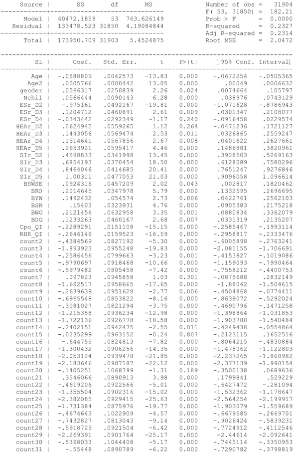
Table 1

regress SL Age Age2 gender Nchil ESr_D* HEAr_D* SIr_D* BSWSE BRO BYW BSR BWG BOG Cpo_QI RHR_QI count*

Source | SS df MS Number of obs = 31904 ---+--- F( 53, 31850) = 182.21 Model | 40472.1859 53 763.626149 Prob > F = 0.0000 Residual | 133478.523 31850 4.19084844 R-squared = 0.2327 ---+--- Adj R-squared = 0.2314 Total | 173950.709 31903 5.4524875 Root MSE = 2.0472

--- SL | Coef. Std. Err. ---+--- Age | -.0588809 .0042573 Age2 | .0005766 .0000442 gender | .0566317 .0250839 Nchil | .0566444 .0090143 ESr_D2 | -.975161 .0492167 ESr_D3 | .1204712 .0460891 ESr_D4 | -.0343442 .0292349 HEAr_D2 | .0624945 .0559265 HEAr_D3 | .1443056 .0569474 HEAr_D4 | .1514641 .0567856 HEAr_D5 | .2653921 .0595417 SIr_D2 | .4598833 .0341998 SIr_D3 | .6854193 .0370454 SIr_D4 | .8464046 .0414685 SIr_D5 | 1.00311 .0477053 BSWSE | .0924316 .0457209 BRO | .2014645 .0347978 BYW | .1492432 .054574 BSR | .15403 .0323931 BWG | .2121456 .0632958 BOG | .1233263 .0460167 Cpo_QI | -.2289291 .0151108 RHR_QI | -.2646146 .0159523 t P>|t| [95% Conf. Interval] -13.83 0.000*** -.0672254 -.0505365 13.05 0.000*** .00049 .0006632 2.26 0.024** .0074664 .105797 6.28 0.000*** .038976 .0743129 -19.81 0.000*** -1.071628 -.8786943 2.61 0.009*** .0301347 .2108077 -1.17 0.240 -.0916458 .0229574 1.12 0.264 -.0471236 .1721127 2.53 0.011** .0326865 .2559247 2.67 0.008*** .0401622 .2627661 4.46 0.000*** .1486881 .3820961 13.45 0.000*** .3928503 .5269163 18.50 0.000*** .6128089 .7580296 20.41 0.000*** .7651247 .9276846 21.03 0.000*** .9096058 1.096614 2.02 0.043** .002817 .1820462 5.79 0.000*** .1332595 .2696695 2.73 0.006*** .0422761 .2562103 4.76 0.000*** .0905383 .2175218 3.35 0.001*** .0880834 .3362079 2.68 0.007*** .0331319 .2135207 -15.15 0.000*** -.2585467 -.1993114 -16.59 0.000*** -.2958817 -.2333476

Statistically significant at 95% (**), and 99% (***).

From the results in Table 1 we can conclude that only educational level “2” and

employment status “4” are not statistically significant meaning that, ceteris paribus, having

completed elementary education does not add (statistically speaking, and even with the positive

sign on HEAr_D2) to one’s satisfaction with life (in comparison with not having completed that

18

(12)

educational level). Having “other employment” status, rather than being employed full-time,

(when one is neither unemployed nor a housewife) is statistically irrelevant in changing one’s

satisfaction with life (although the sign is negative).

All other variables are statistically significant at 99% of confidence (only BSWSE,

HEAr_D3 and gender are statistically significant at 95% of confidence) and all present the

expected sign according to our hypothesis and the literature19_.

Trying to grasp now the relative importance of the independent variables (and grouping

them by their type: economic domain, social capital, quality of institutions and

socio-demographics) in explaining SL, the main results are the following:

The results for the controls (the socio-demographic variables) are in line with the robust

results in the literature: SL is U-shaped in age20, women are slightly happier than men (more

0.057 satisfaction points)21 and being unemployed (in contrast with having a full-time job)

drastically diminishes one’s satisfaction with life (a 0.98 points drop). Concerning education, our

results show that having higher education contributes to one’s satisfaction (having attended

university in comparison with not having completed elementary education adds 0.27 point on our

satisfaction)22.

With regard to the other broad determinants of happiness (social capital and quality of

institutions in comparison with economic wellbeing), the economic domain (SIr) seems to have a

similar impact on one’s satisfaction with life as that of the perception of institutions’ quality, and

its impact is only a little bit greater than that of social capital levels. Belonging to the 5th level of

the scale of incomes (in comparison with being at the bottom of that scale) adds roughly 1 point

in our satisfaction with life. That means that (on average) for each jump on the SIr we get

approximately 0.25 satisfaction points. That is also the impact of the quality of institutions (0.23

satisfaction points for each point in confidence gain for the police and 0.26 for each point more

on the perception of respect for human rights) and similar to that of social capital variables

(minimum for BSWSE with 0.09 satisfaction points gain and maximum for BWG with 0.21).

19

Note that Cpo_QI assumes the value 1 for “a great deal” and 4 for “none at all” and RHR_QI assumes 1 for “there is a lot of respect for human rights” and 4 for “there is no respect at all” which explains the negative coefficients. 20_{Although this is an expected result it should be pointed out that a cross section analysis is not the ideal way to} analyze the life cycle evolution of happiness. A better analysis of the life cycle evolution of happiness was done by Easterlin (2006).

21

This is also in line with some earlier empirical literature, e.g. Di Tella et al. (2001). 22

(13)

This means that besides the already expected importance of money on ones’ satisfaction

with life, participating in social organizations (that is, displaying a higher level of social capital)

and having a perception of living in a fair and safe society are as important for one’s well-being.

Having proceeded with the HEAr and ISr decomposition into dummies, we can now

evaluate the change in the marginal effects of these two variables: by subtracting consecutively

the dummies’ coefficients, we can access the impact of changing from one level to the next on

both income and education. Table 2 reports these results:

Table 2

variable coefficient marginal effect D2 0.06249 0.06249 D3 0.1443 0.08181 D4 0.1515 0.0072 HEAr

D5 0.2654 0.1139 D2 0.4599 0.4599 D3 0.6854 0.2255 D4 0.8464 0.161 SIr

D5 1.0031 0.1567

We can see that the changes in the marginal effects are different for education and

income. While income presents a clear pattern of diminishing marginal effect (moving from

income level 1 to 2 adds much more to one’s SL than moving from level 4 to 5)23, education

exhibits a somewhat irregular pattern with the step from having completed secondary education

to having university frequency (from 4 to 5) being the most relevant step of all. On the other

hand, completing secondary education or not completing it (from 3 to 4) is almost irrelevant

from a SL point of view.

Overall we may conclude that material well-being is an important determinant of happiness

(though with diminishing marginal utility), but the perception of the quality of institutions has a

similar relevance and social ties come third in relevance. This implies that they should be taken

into account when evaluating individuals’ welfare and policies to improve it.

23

(14)

5. Analysis with country-level data

In the previous section we only took account of countries to get rid of possible countries’

fixed effects and not to derive country specific conclusions. This section fills the gap, and we

address the determinants of average life satisfaction (SL) across countries.

Our aim is also to study the impact of social capital, quality of institutions and the

economic environment on happiness. We want to test the same relations as those previously

tested in the Micro model using fewer and slightly different variables because we have fewer

degrees of freedom24. The unemployment rate (Unem), inflation (Inf) and the logarithm of Gross

Domestic Product per capita and at purchasing power parity (lnGDP) are the alternative

indicators of the economic environment.25 Average confidence in police (Cpo_QI) and a

compilation of governance quality (GovDo26) are the indicators of institutions’ quality. Finally,

the social capital variable is the simple average of fifteen dummies concerning belonging (or not)

to the fifteen different organizations displayed on the WVS dataset.27

Since SLi is the average satisfaction with life for country i, we are dealing with a

continuous variable in the interval [0,10]. Therefore, we can also use ordinary least squares for

estimation of the following equations28:

Economic Well-Being:

MaM1 - SL_i =b₀+b₁lnGDP_i+u_i

MaM2 - SL_i =b₀+b₁lnGDP_i +b₂Unem_i +b₃Inf_i +u_i

Quality of Institutions:

MaM3 - SL_i =b₀+b₁Cpo_QI_i+u_i

MaM4 - SL_i =b₀+b₁GovDo_i+u_i

MaM5 - SL_i =b₀+b₁Cpo_QI_i+b₃GovDo_i+u_i

24

The equations are grouped according to the type of variables used. To be parsimonious (because now with only 32 data points (countries) we are working with much fewer degrees of freedom), we have only selected three variables for economic environment, two for the quality of institutions and one for social capital.

25

Previous literature has found a nonlinear relationship between GDP and happiness (e.g. Helliwell and Huang (2008).

26

GovDo is the simple average of the percentile rank of each country on four dimensions of governance quality as measured by the Worldwide Governance Indicators project (Kaufmann, Daniel), to wit, Government Effectiveness, Regulatory Quality, Rule of Law and Control of Corruption.

27

In brackets the chosen abbreviation used in Stata. As previously, the year used for each country can be seen in Table 4 in the appendix. Also in the appendix is Table 7 with these variables’ descriptive statistics. These variables are aggregations for each country. For the variables from the WVS, the country’s average is used.

28

(15)

Social Capital:

MaM6 - SL_i =b₀+b₁belong_i+u_i

Global Models:

MaM7 - SL_i =b₀+b₁lnGDP_i+b₂Unem_i+b₃Inf_i+b₄Cpo_QI_i+b₅GovDo_i+b₆belong+u_i

MaM8 - SL_i =b₀+b₁Unem_i+b₂Inf_i+b₄Cpo_QI_i +b₆belong_i+u_i

Once more, b stands for parameters to be estimated and u for the random error term with

the desirable proprieties.

The OLS estimation results are shown in Table 329.

Table 3

MaM1 MaM2 MaM3 MaM4 MaM5 MaM6 MaM7 MaM

L

coef p > |t| coef p > |t| coef p > |t| Coef p > |t| coef p > |t| coef p > |t| coef p > |t| coef p

GDP 1.3347 0.000*** 0.9765 0.002*** 0.9807 0.031**

Unem -0.0732 0.038** -0.0808 0.019** -0.0985 0

Inf -0.0085 0.649 -0.0339 0.108 -0.0417 0

o_QI -1.8359 0.000*** -0.731 0.169 -0.9125 0.052* -0.8785 0

ovDo 4.293 0.000*** 3.2586 0.005*** -2.9914 0.059*

elong 0.7251 0.000*** 0.1941 0.148 0.2393

uared 0.6765 0.728 0.3853 0.5049 0.5366 0.4417 0.7957 0.746

r Obs 32 32 32 32 32 32 32 32

Statistically significant at 90% (*), 95% (**), and 99% (***).

From the analysis of the results we can reinforce the conclusions of our micro analysis:

the effect of both social capital and the quality of institutions is significant alongside the

relevance of economic factors: lnGDP, Cpo_QI, GovDo or belong. All are highly significant

when they are regressed alone over SL. Also the idea that income is the best proxy for

satisfaction with life (once the curvilinear relationship is taken into account by the usage of the

logarithm of income), followed by institutions’ quality and social capital, can be witnessed by

the diminishing R-square once one moves from regression MaM1 (for income) to MaM3 and

MaM4 (for institutions) and to MaM6 (for social capital).

Once we move to the estimation with several variables (MaM7 and MaM8) things

become less clear as some variables lose statistical significance and others change sign: in

MaM7 (where all the variables are included) only lnGDP, Unem and Cpo_QI remain significant

29

(16)

and with the expected sign. However, inflation (Inf) and social capital (belong) lose significance

(although retaining the correct sign) and GovDo remain significant but with the wrong sign.

Only if we do not introduce lnGDP (as in MaM8) do we get the full expected results:

unemployment and inflation contribute negatively to SL, and social capital and quality of

institutions have a positive impact.

Using the sample’s standard deviations of each variable as a reference for a typical

movement of that variable, we can compare the impacts of the different variables on SL. Thus we

find that economic variables have a greater impact on SL (for one SD of unemployment there is a

0,4 point reduction in SL, for one SD of inflation there is a 0,313 point reduction30). The

institutional variables come next: for a SD increase in confidence in police (that is, lower

Cpo_QI), there is a 0,287 gain in SL, and lastly the social capital variable (a SD increase in

belong boosts SL by 0,212 points). This is in line with the results previously found in the micro

analysis, which adds robustness to the present analysis.

6. Conclusions

The empirical evidence presented in this paper seems to support the hypothesis that life

satisfaction is related not only to personal characteristics related to material well-being (e.g.

income scale) and the usual socio-demographic characteristics (women are happier than men and

young people are happier than old people), but also to the perceived fairness of institutions.

Respect for human rights and confidence in the police are related to individual life satisfaction.

This is a further empirical argument in support of a theory of justice. Just institutions are

valuable for the functioning of a “well ordered society”, and citizens in fact seem to value them

and relate better institutions with enhanced life satisfaction. Of lesser importance, but still

relevant, is the density of social networks that the individuals belong to. The higher the

participation in social organizations, the higher the levels of life satisfaction.

These conclusions at the individual level become somewhat blurred at the country level

since variance of country average life satisfaction is much less than intra country variance of

individual life satisfaction. Nevertheless, we still observe that low levels of unemployment and

inflation, high levels of civic participation and high confidence in the police are positively

associated with life satisfaction.

30

(17)

When comparing our results with those in the literature we find some consistency among

results, since it is not just material well-being that counts for happiness. However, it seems that

material well-being is more important than some papers have suggested, particularly when we

take into account that our sample comprised relatively rich countries.

Results from happiness research should be taken into account for public policy, because

they add information for decision-makers on the impact of their policies. However, caution is

advised for several reasons. First, even for a utilitarian decision-maker, the subjective perception

of well-being can only be a rough indicator of happiness. In this case it should be complemented

by other approaches such as time allocation on different activities and the subjective perception

of these experiences. Second, if we depart from the utilitarian approach and join a Rawlsian

approach, what really matters are just institutions. As stated in this paper, they may go hand in

hand, in the sense that fairer institutions seem to bring more happiness overall. But in case of

conflict, a Rawlsian approach gives a clear priority to justice.

References

Bentahm, Jeremy. 1822

Beugelsdijk, Sjoerd. 2006. “A note on the theory and measurement of trust in explaining

differences in economic growth.” Cambridge Journal of Economics, 30, pp. 371-87.

Blanchflower, David G. and Andrew J. Oswald. 2004. “Well-being over time in Britain and the

USA.” Journal of Public Economics, 88, pp. 1359-86.

Bruni, Luigino and Pier Luigi Porta. 2005. Economics and Happiness: Framing the Analysis:

Oxford University Press.

Clark, Andrew and Andrew J. Oswald. 1994. “Unhappiness and Unemployment.” The Economic

Journal, 104:424, pp. 648-59.

Diener, Ed and Eunkook Suh. 1997. “Measuring Quality of Life: Economic, Social, and

Subjective Indicators.” Social Indicators Research, 40, pp. 189-216.

Dolan, P. and M. White. 2007 “How can Measures of Subjective Well-Being be Used to Inform

(18)

Easterlin, Richard A. 2001. “Income and Happiness: Towards a Unified Theory.” The Economic

Journal, 111:473, pp. 465-84.

Easterlin, Richard A. 2006. “Life cycle happiness and its sources: Intersections of psychology,

economics, and demography.” Journal of Economic Psychology, 27, pp. 463-82.

Frank, Robert H. 1997. “The Frame of Reference as a Public Good.” Economic Journal,

107:445, pp. 1832-47.

Frank, Robert H. 2005. “Does Absolute Income Matter?,” in Economics and Happiness:

Framing the Analysis. Luigino Bruni and Pier Luigi Porta eds. Oxford: Oxford University Press.

Frey, Bruno S and Alois Stutzer. 2002. Happiness and Economics: how the economy and

institutions affect human well-being: Princeton University Press, Princeton and Oxford.

Frey, Bruno S. and Alois Stutzer. 2000. “Happiness, Economy and Institutions.” The Economic

Journal, 110, pp. 918-38.

Fukuyama, F. 1995. Trust: Social Virtues and the Creation of Prosperity. New York: Free Press.

Gardner, Jonathan and Andrew Oswald. 2006. “Do divorcing couples become happier by

breaking up?” Journal of the Royal Statistical Society, 196:Part 2, pp. 319-36.

Guiso, Luigi, Paola Sapienza, and Luigi Zingales. 2003. “People's opium? Religion and

economic attitudes." Journal of Monetary Economics, 50, pp. 225-82.

Helliwell, John F. 2004. “Well-being and social capital: does suicide pose a puzzle?”, NBER

Working Paper 10896.

Helliwell, John F. 2006. “Well-Being, Social Capital and Public Policy: What’s New?” The

Economic Journal, 116, pp. C34-C45.

Helliwell, John F. and Haifang Huang. 2008. “ How´s Your Government? International Evidence

Linking Good Government and Well-Being” The British Journal of Political Science, 38,

pp595-619

Kahneman, Daniel.; Alan B. Krueger, D. Schkade, N. Schwarz, and A. Stone, 2004. “Toward

National Well-Being Accounts.” The American Economic Review, 94, pp. 429

Kahneman, Daniel and Alan B. Krueger. 2006. “Developments in the Measurement of

Subjective Well-Being.” Journal of Economic Perspectives, 20:1, pp. 3-24.

Knack, Stephen and Philip Keefer. 1997. “Does Social Capital Have and Economic Payoff? A

(19)

Konow, J. and J. Earley. 2008. “The Hedonistic Paradox: Is Homo Oeconomicus Happier?”

Journal of Public Economics, 92, p. 1-33

La Porta, Rafael, Florencio Lopez-de-Silanes, Andrei Shleifer, and Robert W. Vishny. 1997.

“Trust in Large Organizations.” The American Economic Review, 87:2, pp. 333-38.

Layard, Richard. 1980. “Human Satisfaction and Public Policy.” Economic Journal, 90, pp.

737-50.

Layard, Richard. 2005a. Happiness: Lessons from a New Science: The Penguin Press, New

York.

Layard, Richard. 2005b. “Rethinking Public Economics: The Implications of Rivalry and Habit,”

in Economics and Happiness: Framing the Analysis. Luigino Bruni and Pier Luigi Porta eds.

Oxford: Oxford University Press.

Ng, Yew-Kwang. 1978. “Economic Growth and Social Welfare: The Need for a Complete Study

of Happiness.” Kyklos, 31:4, pp. 575-87.

Ng, Yew-Kwang. 1997. “A Case for Happiness, Cardinalism, and Interpersonal Comparability.”

Economic Journal, 107:445, pp. 1848-58.

Ng, Yew-Kwang. 2001. “Is Public Spending Good for You?” World Economics, 2:2, pp. 1-17.

Ng, Yew-Kwang. 2003. “From Preference to Happiness: Towards a more Complete Welfare

Economics.” Social Choice and Welfare, 21, pp. 113-116.

Ostrom, E. and T. K. Ahn, (eds.) 2003. Foundations of Social Capital, Edward Elgar,

Cheltenham, UK

Oswald, Andrew. 1997. “Happiness and Economic Performance.” Economic Journal, 107:445,

pp. 1815-31.

Putnam, R. 2000, Bowling Alone. The Collapse and Revival of American Community. New York,

Simon and Schuster

Putnam, Robert, Robert Leonardi, and Raffaella Y. Nanetti. 1993. Making Democracy Work:

Civic Traditions in Modern Italy: Princeton University Press.

Rawls, John, 1996. Political Liberalism,

Rawls, John. 1971. A Theory of Justice: Belknap Press.

Slemrod, Joel and Peter Katuscák. 2005. “Do Trust and Trustworthiness Pay Off?” The Journal

(20)

Di Tella, Robert, Robert J. MacCulloch, and Andrew J. Oswald. 2001. “Preferences over

Inflation and Unemployment: Evidence from Surveys of Happiness.” The American Economic

Review, 91:1, pp. 335-41.

Torgler, Benno. 2005. “Tax morale in Latin America.” Public Choice, 122, pp. 133-57.

Van Praag, Bernard and Ada Ferrer-i-Carbonell. 2004. Happiness Quantified: A Satisfaction

Calculus Approach. New York: Oxford University Press.

Veenhoven, Ruut. 1999. “Quality of Life in Individualistic Society: A comparison of 43 nations

in the early 1990's.” Social Indicators Research, 48, pp. 157-86.

Veenhoven, Ruut. 2002. “Why Social Policy Needs Subjective Indicators.” Social Indicators

(21)

Appendix

Table 4 (code on WVS in brackets)

Code Country (s003) Year (s020) Wave

40 austria 1999 4

56 belgium 1999 4

100 bulgaria 1999 4

124 canada 2000 4

191 croatia 1999 4

203 czech republic 1999 4

208 denmark 1999 4

233 estonia 1999 4

246 finland 2000 4

250 france 1999 4

276 germany 1999 4

300 greece 1999 4

348 hungary 1999 4

352 iceland 1999 4

372 ireland 1999 4

380 italy 1999 4

392 japan 2000 4

428 latvia 1999 4

440 lithuania 1999 4

442 luxembourg 1999 4

484 mexico 2000 4

528 netherlands 1999 4

616 poland 1999 4

620 portugal 1999 4

642 romania 1999 4

703 slovakia 1999 4

705 slovenia 1999 4

724 spain 1999.5 4

752 sweden 1999 4

792 turkey 2001 4

826 great britain 1999 4

(22)

Table 5 - Table 1 including estimation results of country dummies

regress SL Age Age2 gender Nchil ESr_D* HEAr_D* SIr_D* BSWSE BRO BYW BSR BWG BOG Cpo_QI RHR_QI count*

Source | SS df MS Number of obs = 31904 ---+--- F( 53, 31850) = 182.21 Model | 40472.1859 53 763.626149 Prob > F = 0.0000 Residual | 133478.523 31850 4.19084844 R-squared = 0.2327 ---+--- Adj R-squared = 0.2314 Total | 173950.709 31903 5.4524875 Root MSE = 2.0472

(23)

_cons | 9.4477 .1323504 71.38 0.000 9.188288 9.707111 ---

Table 6 - Micro model estimated by ordered logit, including country dummies

Ordered logistic regression Number of obs = 31904 LR chi2(53) = 8085.86 Prob > chi2 = 0.0000 Log likelihood = -63165.416 Pseudo R2 = 0.0602

(24)

/cut1 | -5.960832 .1219982 -6.199944 -5.72172 /cut2 | -5.455454 .1205672 -5.691762 -5.219147 /cut3 | -4.800943 .1193098 -5.034786 -4.5671 /cut4 | -4.300195 .1186136 -4.532674 -4.067717 /cut5 | -3.498383 .1177734 -3.729214 -3.267551 /cut6 | -2.947363 .1173311 -3.177327 -2.717398 /cut7 | -2.181127 .1168713 -2.410191 -1.952064 /cut8 | -1.035976 .1164622 -1.264238 -.8077147

/cut9 | -.1025429 .1165506 -.3309778 .1258921

--- Table 7 - Descriptive Statistics for the variables used on the Micro Model: Variable | Obs Mean Std. Dev. Min Max ---+--- SL | 31904 6.968186 2.335056 1 10

Age | 31904 44.75135 16.66648 15 98

gender | 31904 .5253573 .4993644 0 1

Nchil | 31904 1.730943 1.551914 0 20

ESr_D2 | 31904 .0678912 .251563 0 1

---+--- ESr_D3 | 31904 .101492 .3019838 0 1

ESr_D4 | 31904 .4132397 .4924228 0 1

HEAr | 31904 3.43098 1.195364 1 5

SIr | 31904 2.686685 1.27571 1 5

BSWSE | 31904 .0749122 .2632538 0 1

---+--- BRO | 31904 .1785983 .3830216 0 1

BYW | 31904 .0514042 .2208242 0 1

BSR | 31904 .1805103 .3846179 0 1

BWG | 31904 .03708 .1889608 0 1

BOG | 31904 .0706494 .2562424 0 1

---+--- Cpo_QI | 31904 2.372367 .8402523 1 4

RHR_QI | 31904 2.313534 .8207859 1 4

Table 8 – Description of HEAr and ESr

HEAr - highest educational level attained r

Level - Meaning

--- 1 - inadequately completed elementary education |

2 - completed (compulsory) elementary education |

3 - incomplete secondary school: technical/ incomplete secondary: university-preparatory | 4 - complete secondary school: technical/vocational/ complete secondary: university-preparatory | 5 - some university without degree/higher e university with degree/higher education |

---ESr – employment status r Number - Employment status |

--- 1 - full time |

2 - unemployed | 3 - housewife |

4 - other / part time / self employed / students / retired | ---

(25)

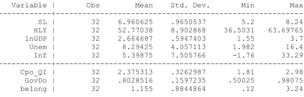
Table 9 – Descriptive statistics for the variables used on the Macro Models (31 countries):

Table 10 – Correlation matrix for the variables used on the Macro Models

| SL HLY lnGDP Unem Inf Cpo_QI GovDo belong ---+--- SL | 1.0000

HLY | 0.9854 1.0000

lnGDP | 0.8225 0.8873 1.0000

Unem | -0.6630 -0.6433 -0.5871 1.0000

Inf | -0.4380 -0.5007 -0.6045 0.0263 1.0000

Cpo_QI | -0.6208 -0.6360 -0.6468 0.4443 0.1151 1.0000

GovDo | 0.7105 0.7708 0.9136 -0.5319 -0.5887 -0.6927 1.0000

belong | 0.6646 0.6849 0.6303 -0.4946 -0.3139 -0.4673 0.5839 1.0000

Table 11 – Estimation results for the Macro Models

OLS Estimation of MaM1 regress SL lnGDP

Source | SS df MS Number of obs = 32 ---+--- F( 1, 30) = 62.74 Model | 19.5322182 1 19.5322182 Prob > F = 0.0000 Residual | 9.33896873 30 .311298958 R-squared = 0.6765 ---+--- Adj R-squared = 0.6657 Total | 28.8711869 31 .931328611 Root MSE = .55794

--- SL | Coef. Std. Err. t P>|t| [95% Conf. Interval] ---+--- lnGDP | 1.334651 .1684925 7.92 0.000 .9905429 1.678758 _cons | 3.404198 .4596858 7.41 0.000 2.465395 4.343002 ---

OLS Estimation of MaM2 regress SL lnGDP Unem Inf

(26)

---

OLS Estimation of MaM3 regress SL Cpo

--- SL | Coef. Std. Err. t P>|t| [95% Conf. Interval] ---+--- Cpo_QI | -1.835942 .423343 -4.34 0.000 -2.700524 -.9713607 _cons | 11.32156 1.014722 11.16 0.000 9.249224 13.3939

OLS Estimation of MaM4 regress SL GovDo

--- SL | Coef. Std. Err. t P>|t| [95% Conf. Interval] ---+--- GovDo | 4.293041 .7762282 5.53 0.000 2.707771 5.87831 _cons | 3.513951 .6350311 5.53 0.000 2.217044 4.810857 ---

OLS Estimation of MaM5 regress SL Cpo GovDo

--- SL | Coef. Std. Err. t P>|t| [95% Conf. Interval] ---+--- Cpo_QI | -.7309542 .5183963 -1.41 0.169 -1.791194 .3292853 GovDo | 3.258584 1.059031 3.08 0.005 1.092623 5.424545 _cons | 6.08071 1.924606 3.16 0.004 2.144448 10.01697 ---

OLS Estimation of MaM6 regress SL belong

(27)

---

OLS Estimation of MaM7

regress SL lnGDP Unem Inf Cpo GovDo belong

OLS Estimation of MaM8

regress SL Unem Inf Cpo belong