Inequality and economic growth in Latin
*Lilian Furquim and Fernando Garcia**
Abstract
Latin America is the region that bears the highest rates of inequality in the world. Deininger and Squire (1996) showed that Latin American countries achieved only minor reductions in inequality between 1960 and 1990. On the other hand, East Asian countries, recurrently cited in recent literature on this issue, have signifi-cantly narrowed the gap in income inequality, while achieving sustained economic growth. These facts have triggered a renewed discussion on the relationship between income inequality and economic growth. According to the above literature, income inequality could have an adverse effect on countries’ growth rates. The main authors who spouse this line of thinking are Persson and Tebellini (1994), Alesina and Rodrik (1994), Perotti (1996), Bénabou (1996), and Deininger and Squire (1996, 1998). More recently, however, articles were pub-lished that questioned the evidence presented previously. Representatives of this new point of view, namely Li and Zou (1998), Barro (1999), Deininger and Olinto (2000) and Forbes (2000), believe that the relation between these variables can be positive, i.e., income inequality can indeed foster economic growth.
Using this literature as a starting point, this article seeks to evaluate the relation between income inequality and economic growth in Latin America, based on a 13-country panel, from 1970 to 1995. After briefly reviewing the above articles, this study estimates the per capita GDP and growth rate equations, based on the neoclassical approach for economic growth. It also estimates the Kuznets curve for this sample of countries. Econometric results are in line with recent work conducted in this area – particularly Li and Zou (1998) and Forbes (2000) – and confirm the positive relation between inequality and growth, and also support Kuznets hypothesis.
Key words: Income inequality, economic growth, Kuznets curve, Latin America.
JEL Classification: O15, O40.
1 Introduction
Latin America is the region that bears the highest rates of inequality in the world.
Dein-inger and Squire statistics (1996), shown in table 1, attest that Latin American countries
consis-tently had the highest rates of inequality between 1960 and 1990. While most other regions –
notably East Asian countries – managed to significantly reduce inequality indicators from 1970
to 1990, income inequality remained high in Latin America.
The huge income inequality is associated to education distribution in the region,
ac-cording to the Interamerican Development Bank – IDB (1998)1. The richest inhabitants of each
country are also the most educated, since they have opportunity to graduate from high school
and enter universities. In Latin America, education distribution follows the same pattern of
income distribution. Income differences can largely be explained by education differences, as
*
The authors wish to acknowledge the help provided by Ramón Fernandez, Yoshiaki Nakano, Arthur Barrionuevo and Marcos Gonçalves da Silva in preparing this study. Nevertheless, any remaining errors or omissions are the full responsibility of the authors.
illustrated by graph 1 below. Estimates based on IDB data (1998)2, which consider the partic
i-pation in the product according to deciles in income distribution and average education of each
group, for a set of 14 economies in the mid 90s, indicate that a typical Latin American citizen
can increase his or her annual income by an average of 12%, for each additional year of
schooling. Since a wide gap in education exists, income inequality is an inevitable consequence.
Table 1 Gini index according to regions, 1960 to 1990
Region 1960 1970 1980 1990
Latin America and Caribbean 53.2 49.1 49.7 49.3
Sub-Saharan Africa 49.9 48.2 43.5 46.9
Middle East and North Africa 41.4 41.9 40.4 38.0
East Asia and Pacific 37.4 39.9 38.7 38.1
South Asia 36.2 33.9 35.0 31.9
Industrialized and Developing Countries 35.0 34.8 33.2 33.7
East Europe 25.1 24.6 25.0 28.9
Source: Deininger and Squire (1996).
Graph 1 Income and education according to income distribution deciles, Latin America, mid 90s.
Anos de escolaridade
8 6
4 2
0 -2
-4
Renda per capita do decil (ln)
3
2
1
0
-1
-2
-3
Source: own calculations based on IDB statistics (1998).
1 Asset distribution, as well as land distribution, are decisive factors in explaining inequality. See IDB (1998). 2 These estimates consider a panel with 10 observations (income-distribution deciles) for each of the 14 economies.
According to Birdsall et al (1995), education was the main variable behind the sustained
growth enjoyed by East Asian countries. Public policies aimed at the expansion of the education
basis improved education distribution among inhabitants of these countries, consequently
af-fecting productivity and narrowing income inequality. Thus, policies ensured that the fruit of
growth could be distributed, fostering subsequent growth.
Literature on income inequality and economic growth published in the 90s considers
East Asian countries classic examples, since they achieved considerable growth and narrowed
their income gaps. This fact triggered renewed discussions regarding the relation between
in-come inequality and economic growth and rekindled discussion on the Kuznets hypothesis – an
inverted-U-shaped relation between per capita income and its distribution. According to this
literature, income inequality could negatively affect a country’s growth rates. The main studies
that spouse this line of thinking are the following: Persson and Tabellini (1994), Perotti (1993),
Alesina and Rodrik (1994), Bénabou (1996), Clarke (1995), Alesina and Perotti (1994), and
Panizza (1998). More recently, however, another set of articles questioned the findings of the
first line of studies. Li and Zou (1998), Barro (1999), Deininger and Olinto (2000), and Forbes
(2000), discuss, based on new empirical evidence, if in fact inequality has negative impact on
the rate of economic growth. These authors, unlike the previous ones, found a positive relation,
meaning that income inequality can indeed benefit growth.
This article aims to evaluate the relation between income inequality and economic
growth in Latin America, considering the period between 1970 and 1995. To do so, this article
is divided into three sections, in addition to this introduction. The first summarizes recent work
published on this issue, pointing out theoretical aspects and explanations for this set of studies.
The second presents a series of regressions, which evaluate the relation between inequality and
growth in Latin America, based on the neoclassical economic growth theory and on the Kuznets
curve specifications. The third briefly discusses this article’s findings and how they fit into the
recent literature on the subject.
2 A review of the literature on inequality and economic growth
In the 90s much work was produced focusing the growth area, particularly regarding
distribution issues. The resumption of the inequality theme was fueled mainly by the
perform-ance of Asian countries in the last three decades3. As pointed out by the 1993 World Bank
Re-port:
3
“Some countries in East Asia sustained per capita GDP growth rates of 4-5 percent
over four decades, with massive improvements in living standards and in health and
education for poor people and for everyone else” (World Bank Report, 2000, p. 35)
These facts motivated several researchers to evaluate whether the reduction in income
inequality was a decisive factor in that region’s economic performance. A pioneering study
evaluating the relation between inequality and growth was that of Persson and Tabellini (1994).
The authors created a theoretical model, which related income inequality and growth using
po-litical mechanisms. Generally speaking, societies with wide income gaps do not protect
prop-erty rights and do not allow full appropriation of returns on investments. Such facts choke
capi-tal accumulation and consequently economic growth. This first article was followed by a series
of studies on this subject, summarized by Bénabou (1996), which compiles 23 theoretical and
empirical works on inequality, economic growth and investment4. Among the chief conclusions
of the works summarized by Bénabou (1996) are the following:
“[...] a one standard deviation decrease in inequality raises the annual growth rate of
GDP per capita by .5 to .8 percentage points.” (p. 2)
”[...] In any case, enrollments in and stocks of secondary education have a substantial
negative correlation with inequality, and in some of the theories discussed below the
link between income distribution and growth arises precisely through human capital
investment.”(p.3)
To ease exposition and analysis of the models relating inequality and growth, the studies
were classified according to the key mechanism pointed out by the authors. Much work, such as
that of Barro (1999), Rodríguez (2000), Deininger and Olinto (2000), Ferreira (1999), and
Perotti (1996), aim at such classification5. The most comprehensive is that developed by
Dein-inger and Olinto (2000), which states that there are three main lines of work: (i) models of
po-litical economics; (ii) models of imperfections in the credit market and indivisible investments;
and (iii) models of social unrest and economic efficiency. Below are the main works in each
area. At the end, there are some other studies not fitting this classification.
2.1 Political economics models
The works in this first group6 can be further divided into two categories: the first was
in-spired by Meltzer and Richard (1981) and the second resulted from flaws in the empirical
4 No empirical works are analyzed in this section, although some of those works will form the comparison basis for
the empirical tests results developed in this article. For a summary of the works, see Bénabou (1996) and Durlauf and Quah (1998).
5
Please see the summary of the approaches suggested by Aghion et al (1999).
6
evaluation performed by the first one. Essentially, this work is grounded on the notion of the
redistributive role of the State. Governments tax income, according to the proportional taxation
principle, and then redistribute the proceeds in egalitarian form. Given that taxation is decided
by the median voter, if the income of this particular economic agent is below the population’s
average income, he or she will decide to raise taxes and consequently redistribute the income
earned by these taxes. Therefore, if inequality is measured as the distance between the median
voter and the mean voter, high inequality will lead to greater taxation, which will affect
invest-ment decisions. Taxation and redistribution are considered distortive policies that jeopardize
economic efficiency. That is the reasoning behind greater inequality having a negative effect on
growth7.
Persson and Tabellini (1994) argue that in societies where distributive conflicts are
sig-nificant, political decisions can restrain private appropriation of the results of individual effort,
which in turn discourages productive investment and reduces growth. The authors adopted the
superposed generations model, in which individuals born in each period are economic and
po-litical agents (voters). In this model, majority-driven redistribution policies would bring a
nega-tive relation between inequality and income. However, after testing the mechanisms that should
link inequality to growth, for a sample comprised of only OECD nations, it was found that
ine-quality only affects investment in democracies and no significant relation was found between
income redistribution and growth. The results fail to confirm the relation between inequality and
growth, through income redistribution. The authors also point out that empirical results are not
as robust when controlled by regional variables and different political regimes.
Alesina and Rodrik (1994) also establish a relation between income distribution and
growth occurring through distributive policies. The key point is that individuals differ in the
relative endowment of productive factors – capital and work. Growth is determined by
accu-mulation of physical capital, which in turn is determined by individual saving decisions. Go
v-ernment services are financed by taxes on work. Since individuals have different endowments,
preference for different taxation levels will fluctuate among them. For an individual, the lower
the share of his or her income originating from capital, relative to labor income, the greater the
tax rate for such individual, consequently reducing the savings rate and in turn economic
growth. In this model, different from that of Persson and Tebellini (1994), taxes play more than
a redistributive role: they are used for the production of public assets, necessary for private
7
duction. Capital also has a broader role, since it includes all assets, such as physical, human and
technological capital. The core point of the empirical analysis is that the authors, considering
the initial income level and human capital, found a negative relation between income distrib
u-tion, given by the Gini index, and growth. In other regressions the authors used a dummy for
democracy, in order to identify the distinct relation between inequality and income for different
political regimes. They also tested the formulation for land distribution (Gini-land) and
con-cluded that countries that underwent agrarian reform after the war enjoyed higher growth than
those that did not. The examples provided are those of Asian countries, compared to Latin
American ones.
Alesina and Perotti (1994) underline the need to precisely define the notion of
democ-racy. According to the authors, a democracy can be defined as a nation with free, periodical and
multiparty elections, or a society that provides enough civil liberties to its population. In the
empirical analysis, they explore the well-known Gastill civil-liberties index. The results do not
show a relation between democracy and growth, which can be justified by the difficulty of cla
s-sifying regimes, due to the diversity found in the group of non-democratic nations, as opposed
to the relative similarity found in the group of democratic ones. Nonetheless, Barro (1991)
ar-gues that civil liberties have a beneficial effect on a country’s economic performance.8
Deininger and Squire (1998) also tested the influence of different political regimes,
di-viding the sample of countries into democracies and non-democracies9. The authors found
unique results: initial inequality affects only the growth of non-democratic nations. However,
according to the theory, inequality should also affect the growth of democratic ones.10
One work that drifts slightly away from this article’s line of study, but points towards a
direction opposite to the empirical results found hitherto, is that of Rodrik (2000). The author
covers the type of institutions that allow better economic performance11. Rodrik questions the
frail results on the role of democracies in economic performance. According to this author,
par-ticipatory political regimes lead to growth of higher quality – more egalitarian. Econometric
results are partly explained because countries recording the highest growth rates in the last
dec-ades are authoritarian. On the other hand, the author finds that growth rate variance is smaller
in countries with greater political participation. Moreover, in democracies and in nations with
8 Regarding political regimes and growth, see also Durham (1999). 9
Countries with a Gastill index of civil liberties below 2 were considered democratic.
10 Similar results were also found by Clarke (1995) and Alesina and Rodrik (1994).
11 Chong and Calderon (2000) also study the role of the quality of the institutions in economic performance. They
participatory institutions, the response to adverse shocks comes faster. This happens because
this type of adjustments require the management of social conflicts and democracies are natural
breeding grounds for institutions prepared to arbitrate such conflicts. This is precisely why
South Korea and Thailand, nations whose regimes allow greater political participation, better
managed the financial crises they met, unlike Indonesia, a country whose regime curbs political
participation. The author also identifies a significant relation between the extension of political
participation and wages, not disregarding differences in productivity, income level and other
growth determinants.
Rodríguez (2000) argues that no satisfactory empirical evidence exists regarding the fact
that inequality is associated to income redistribution or that redistribution is associated to lower
growth rates12. The Meltzer and Richard model (1981), according to Rodríguez (2000),
consid-ers that the vote for income redistribution occurs in a democratic political environment13.
There-fore, this model would not be suited to describing the economic growth and the expansion of
inequalities in non-democratic regimes.
The second category of studies in this first group14 aims at filling the blanks left by the
first category. To do so, it considers a more complex interaction between income distribution
and growth. Most of this work finds a positive correlation between fiscal policy variables and
growth and, under certain conditions, unequal societies can present lower growth According to
Panizza (1998), in spite of the model’s structure being similar to that suggested by Persson and
Tabellini (1994) as well as Alesina and Rodrik (1994), the negative relation between growth
and inequality is identified in a different form.15
2.2 Models with imperfections in the investment and capital market
Models with imperfections in the investment and capital market comprise the second
group of studies. Generally speaking, in societies will ill-distributed income, the possibilities for
investment in physical and human capital are smaller. The reduction in economic growth is
caused by more limited investment, which in turn is brought by imperfections in the asset ma
r-ket. This literature is based on the work of Loury (1981), who believes that credit restrictions
12
Bénabou (2000) blends a theory of inequality and social contract to solve some issues in the aforementioned literature. According to the author, among the group of industrialized democratic nations, those more unequal tend to distribute less. In this aspect, the author compares the United States with Western Europe, and East Asian coun-tries with Latin American ones. In spite of other differences, both Europe and Latin America are unequal societies.
13 For other comments, see Rodríguez (2000) pp 4-5, Perotti (1994) and Alesina and Rodrik (1994). 14 Acemoglu and Robinson (1996), Bourguinon and Verdier (1996) and Bénabou (1996)
15
prevent the poor from reaching an efficient investment amount, which demands a minimum
sum to run a business. Galor and Zeira (1993) as well as Aghion and Bolton (1997) underscore
the problem of minimum scale, or size of project. In the opinion of Ferreira (1999), p.11:
“[…] this could be a school or college fee; it could be the price of the smallest viable
plot of land in an agricultural community; or the permit to operate a stall in a market.
Wherever you look, the argument goes, you can find people who would be engaged in
a more productive activity, had they only had the minimum initial “investment”
re-quired to enter it.”
Deininger and Olinto (2000) state that this group of studies relate the initial wealth
dis-tribution to growth, based on credit-market imperfections: only entrepreneurs with considerable
personal wealth are able to finance their projects. Because of scarce credit availability, creditors
need guarantees to provide loans. Considering that investments are indivisible, i.e., there are
high fixed costs per project, wealth distribution will determine how many people can finance
their projects16. Investments in education or accumulation of human capital are examples of this
rationale, particularly when no other forms of financing are available. Thus, according to
Dein-inger and Olinto (2000), p.7:
“In the presence of financial market imperfections, countries with different distribution
of wealth (and initial wealth level) will follow different growth paths and may
con-verge to different steady states”
This argument can be used to better understand the endurance, along many generations,
of income inequality, particularly in Latin American countries, where wealth inequality would
block accumulation of human capital, leading to a relative scarcity of skilled labor.17
Bénabou (1996) presents a model that includes imperfect-market and political econo
m-ics models. This author’s model springs from the idea that the income of the decisive voter is
above that of the median voter. Under these circumstances, if inequality is too blatant, the cost
of a redistribution for individuals with higher economic and political power will increase. Under
this perspective, the higher the inequality the smaller the chance to have a income redistribution
policy. Economic growth would be negatively impacted by inequality since, given
credit-market imperfections, asset allocation would not be as efficient as that found in a more
egali-tarian society, where the poor would have a chance to invest in productive activities. Incomplete
asset markets coupled with liquidity restrictions would in this particular case be positive for
16
Aghion and Bolton (1997).
17
growth. In the Rodríguez model (1999b), high inequality shifts assets to rent-seeking activities
and to the securing of political favors18, which choke productive activities.
Regarding the Bénabou (1996) model, Deininger and Olinto (2000) argue that if tax
revenues were not used in consumption, but rather in productive activities or public assets –
such as infrastructure, law and order, citizen protection, property rights assurance and other
expenditures that can not be financed any other way – the impact of inequality on voters would
be harder to predict19. The use of taxes will depend on the nature of the externality involved,
opening the way for many forms of equilibrium20, as well as for changes in inequality with the
intent to avoid revolutions and social disorder (Acemoglu and Robinson, 1998). Moreover,
Deiniger and Olinto (2000) point out that voters are less nearsighted as it is generally believed.
2.3 Models of economic efficiency and social instability
The third group of researchers works with the hypothesis that a politically unstable
envi-ronment has negative effects on investments and therefore lowers growth. The core hypothesis
is that a society with wide income gaps, where political power is likewise concentrated in a
small elite, fuels the discontent of the population. This situation prompts the population to
change the situation through “non-legal” means: disturbances, uprising and predatory activities.
An unstable environment also produces sub-optimum investments, consequently lowering
growth. Moreover, people involved in this type of activity could be engaged in productive
ef-forts. Among the works that support this hypothesis are the following: Alesina and Perotti
(1993, 1994 e 1996), Alesina at alli (1992), Perotti (1994, 1996), and Bénabou (1996).
Alesina and Perotti (1994) provide a list of the articles studying the relation between
growth, inequality and political instability. They point out that the relation between political
instability and growth faces two hurdles: the precise definition of political instability and
en-dogeneity, i.e., the effect of growth on political instability. Social researchers gauge political
instability in two ways. The first is an index comprised of variables such as the number of
pro-tests, murders and revolutions21. The second seeks to identify changes in government and
esti-mates the probability of changes of positions and political parties in the executive branch of
governments22. Thus, the higher this probability the greater is political instability. Another
18
On the effects of corruption over growth, see Mauro (1995). In this work, it is assumed that not only institutions affect growth, but economic variables affect institutions. It finds meaningful results that corruption has a negative effect on investment. It uses a “bureaucracy efficiency” index to measure the quality of the institutions.
19 On this subject, see also Bertola (1993), Cooper (1998), Saint-Paul and Verdier (1994). 20 See Bourguignon and Verdier (1998).
21
Works that have used this measure are: Venieris and Gupta (1986), Barro (1991), Gupta (1990), Mauro (1993), Olzer and Tabellini (1991), and Venieris and Sperling (1989).
22
work, Alesina and Perotti (1996), provides an explanation for political instability. To the
possi-bility of changes in the executive branch, they added the odds of constitutional changes, by way
of electoral processes or illegal methods, such as a coup d'état. For a sample of 71 countries, for
the period between 1960 and 1985, it is found that the most unequal societies are politically
unstable and that such instability has negative effects on growth.23
According to Alesina and Perotti (1994) and (1996), poorer countries are also politically
more unstable. They are unstable because they grow less and they grow less because they are
unstable. Moreover, growth is not influenced solely by the political regime; political instability
is of even greater importance. Transitions from dictatorship to democracy, which are associated
to such instability24, usually occur during periods of low economic growth. Most of the empir
i-cal work in this area has found a positive relation between inequality and instability – Perotti
(1996) being one example. Those who have tested the relation between instability and growth
have also stated that an environment of greater instability will reduce investment and growth.
According to Ferreira (1999), some researchers point out the relation between unequal
societies and high rates of crime, which raises the cost of opportunity to live in such locations.
Much is spent on protection and insurance, thereby reducing the amounts that could be spent on
productive activities. This means that income inequality could be directly associated to the
pro-duction of “public bads” (as opposed to public goods) – violence, criminality and crimes against
property rights, factors which affect growth, whether directly or indirectly. Fay (1993), quoted
in Alesina and Perotti (1994), states that in societies with ill-distributed income, the number of
individuals who perform illegal activities, which threaten property rights, is greater.
2.4 Other approaches
There is a last set of works that does not fit the previous ones discussed but suggests a
relation between income inequality, fertility and education. In this case, investment in human
capital is affected by the fertility rate, which in turn is affected by income distribution. Works
such as that of Becker (1988), Barro and Becker (1988), Becker, Murphy and Tamura (1991),
and Perotti (1996) show that fertility rate is associated to better income distribution, greater
in-vestment in human capital and higher economic growth. This relation is also evaluated in an
environment of credit-market imperfections, where restrictions prevent the poor from investing
in the accumulation of human capital.
23 Barro (1991) uses the frequency of coups d’état and the number of political assassinations to support the idea that
political variables have a negative effect on growth.
24
The work of Lee and Roemer (1998) blends elements of the first and second groups of
studies. It combines the political economics approach with the imperfect credit markets
hy-pothesis. According to the authors, the relation between income inequality and economic
growth is more complex than expressed by the conventional political economics models, i.e.,
those following the formulation of Meltzer and Richard (1981). In the model suggested by Lee
and Roemer (1998), the marginal consumption propensity of the poor is less than that of the
richer. Income inequality affects private investments in two different ways: the first occurs
through taxation on investment, which is the political effect; the second, called the “threshold
effect”, mirrors the result of a minimum scale of investment. According to this last effect,
ine-quality has a positive correlation with private investment, for any tax rate. Therefore, no
nega-tive relation between income inequality and private investment is found, since there are multiple
points of equilibrium, as in Galor and Zeira (1993).
Lastly, Barro (1999) and Rodríguez (2000) highlight the models whose relation between
inequality and growth is positive. Income inequality would concentrate wealth in the hands of
those able to save, the richer. Thus, more inequality would create the necessary assets for
in-vestment and economic growth.
3 Inequality and growth in Latin America – 1970 to 1995
This section aims to evaluate, using econometric exercises, the possible impact of
in-come inequality on the level of product and on the economic growth rate in Latin American
economies from 1970 to 1995. It also aims to estimate the Kuznets curve for this sample of
countries, i.e., if economic growth during that period imposed some behavior pattern to income
inequality. Before commenting the primary data and the econometric methodology employed in
the analysis, it is important to describe the specifications of the product per worker, economic
growth and Kuznets equations used in this article.
3.1 Theoretical specifications
The specifications for the equations for per capita product and its growth followed the
tradition of the Solow model with human capital. The starting point was an aggregated
produc-tion funcproduc-tion, of the Cobb-Douglas type, where the product of each country (Y) is determined by
the stocks of physical capital (K), of human capital (H) and of knowledge (A). In this equation,
the stock of human capital in an economy is defined as the work adjusted to its productivity (h),
which is an increasing function of labor education (u).
α −
α ⋅ ⋅
= 1
) (A H K
where 0<α<1, H =h⋅L e u
e h = φ⋅ .
Based on this equation, the Gini variable is introduced, as an element that adjusts the
productivity of the factors, as suggested by Hall and Jones (1996, 1999), Jones (2000), and
Gar-cia et al (1999) for institutional-type variables – equation (2), where Gini
e
G= . The aim of this
procedure is to capture the effect of inequality on economic efficiency, as suggested by the
theoretical approaches discussed in the previous section.
[
α −α]
γ ⋅ ⋅ ⋅
= 1
) (A H K
G
Y (2)
From equation (2), the specification for the product per effective-human capital unit is
derived, i.e., the production function in its reduced form, where ~y =Y A⋅H , k~ =K A⋅H e
u
e L
H = ⋅ φ.
:
α γ ⋅
=G k
y ~
~ (3)
Solow’s (1956) capital accumulation equation – also expressed in its reduced form –
gives us the conditions for the steady state of the economy. In this equation, sk denotes the
sav-ings rate, n the demographic growth rate, g the technological innovation rate, and d the
depre-ciation rate. k d g n y s
k~& = k.~−( + + ).~ (4)
In the steady-state equilibrium, the variation of the capital stock per unit of
effective-human capital is null, which allows us to calculate the value of the capital stock per unit of
equilibrium effective-human capital, k~*. This value is determined by equation (5). And, by
substituting the value of k~* in the reduced-form production function, the value of the product
per unit of effective-human capital in steady state is obtained, indicated by ~y*and defined by
expression (6). α − α + + = 1 * ~ d g n s
k k (5)
α − α γ + + ⋅ = 1 * ~ d g n s G
y k (6)
By defining y* as the product per worker in steady state, equation (7) is obtained. And,
by linearizing this expression, using the natural logarithm, expression (8) is obtained, which
u
k Ae
d g n s G y φ α − α γ + + ⋅ = . . * 1 (7)
(
n g d)
A us Gini
y k .ln ln .
1 ln . 1 *
ln + + + +φ
α − α − α − α + ⋅ γ = (8)
Assuming the hypotheses of Mankiw, Romer and Weil (1992) regarding knowledge, it
is assumed that At =A0.egt and that ln A(0) = a + ε – where a is a technological constant and ε,
is a specific random shock in the economy. Assuming, by simplification, that t = 0, the empir
i-cal specification to be estimated is obtained, given by equation (9).
(
+ +)
+φ +εα − α − α − α + ⋅ γ +
=a Gini s n g d u
y k .ln .
1 ln . 1 * ln (9)
In equation (9) it is expected that γ be a negative parameter, which would be indicating
that a greater level of inequality, as measured by the Gini income index, would lead the
econ-omy to economic efficiency losses. The higher this coefficient, the greater the impact of
ine-quality on the economy.
Based on equation (9), and assuming that economies drift towards a steady state, it is
possible to deduce in the traditional form the growth equation for the product per worker in this
economy. In addition to the variables which determine the product per worker in steady state, in
the equation that calculates the growth rate, the initial income level per worker emerges as an
explanatory variable.
(
)
(
)
(
)
⋅(
+ +)
+(
−)
φ⋅ +εα − α − − − ⋅ α − α − + ⋅ γ + ⋅ − + = − β − β − β − − β − − u e d g n e s e Gini y e a y y T T k T t T t t 1 ln 1 1 ln 1 1 ln 1 ln
ln 1 1
(10)
Lastly, the Kuznets equation took into consideration the alternate specifications (11) and
(12), which were inspired by previous works, such as those of Deininger and Squire (1998) and
Barro (1999):
( )
+δ ⋅(
(
)
)
+δ ⋅ +ε⋅ δ + δ
= Y L Y L u
Gini 0 1 ln 2 ln 2 3 (11)
(
)
' ' 2 1 ' 1 '0 +δ ⋅ ln −ln +δ ⋅ +ε
δ
= y y− u
Gini t t (12)
3.2 Data bases and econometric methodology
Initially, the sample included 17 countries, studied in the period from 1970 to 1995,
separated into five-year periods, i.e., five time observations for each country: 1970, 1975, 1980,
1985, 1990 e 1995. Following a first evaluation, however, some countries, namely Ecuador,
from lack of information for some years and inequality data presented problems that frustrated
temporal comparison for these economies. Consequently, the 102 observations were reduced to
78, meaning 13 countries analyzed at six points in time. Income distribution was measured by
the Gini index and the main source of information was the data bank provided by Deiniger and
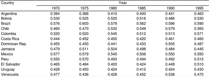
Squire (1996). Inequality data employed are presented in table 2.
Table 2 Gini index for income distribution, Latin America, 1970 to 1995*
Country Year
1970 1975 1980 1985 1990 1995
Argentina 0.394 0.366 0.410 0.400 0.431 0.463
Bolivia 0.530 0.525 0.520 0.516 0.486 0.530
Brazil 0.576 0.603 0.578 0.562 0.596 0.590
Chile 0.460 0.470 0.532 0.549 0.579 0.565
Colombia 0.520 0.520 0.545 0.512 0.513 0.571
Costa Rica 0.444 0.452 0.450 0.420 0.461 0.460
Dominican Rep. 0.455 0.450 0.441 0.433 0.505 0.487
Jamaica 0.479 0.511 0.504 0.498 0.484 0.445
Mexico 0.577 0.579 0.540 0.506 0.550 0.550
Peru 0.550 0.570 0.493 0.494 0.492 0.515
El Salvador 0.465 0.484 0.400 0.424 0.448 0.510
Uruguay 0.428 0.450 0.424 0.412 0.424 0.430
Venezuela 0.477 0.436 0.428 0.452 0.538 0.470
Note: (*) the data refer to the year closest to those shown in the table.
All other variables were built based on World Development Indicators (2000) data. The
measure used as a proxy for human capital – average schooling – was obtained from Barro and
Lee (1996) and updated with information supplied by the Interamerican Development Bank
data bank. Due to the poor quality of the data relative to workforce occupation, it was preferable
to employ the per capita product of these economies and its growth as dependent variables of
equations (9) and (10), respectively, and as independent variables of equations (11) and (12).
It was also assumed that depreciation rate, d, is constant and the same for all countries
comprising the sample, namely 3% per year. The technological innovation rate, g, is also
con-stant and the same for all countries in the sample, by construction. The value assumed was 1.2%
per year, as suggested by Piedrahita (1998), which considers that g is equal to the average per
capita product growth rate in Latin America in the period from 1916 to 1989.
In estimating equations (9) to (12), the Ordinary Least Squares (OLS) method was
em-ployed, since it is assumed that explanatory variables are independent of specific country factors
and also do not depend on residue. According to Mankiw, Romer and Weil (1992) there are
three reasons that justify the independence hypothesis. In addition to this method, the
Two-Stage Ordinary Least Squares method (2OLS) was also employed, to handle eventual
simulta-neity problems between equations (9) and (10), for product per worker and growth rate, and
In both estimation procedures, dummy variables were used to capture the country’s
fixed effects. This procedure aims to capture the effects of the omitted variables, but which
af-fect the per capita product. According to Forbes (2000), p. 5-6:
“Since the dummy variables are significant, this indicates that region-specific factors
affecting growth are not captured by the explanatory variables. Moreover, since the
re-gional variables render the coefficient on inequality insignificant, this suggests that the
coefficient on inequality may actually capture the effect of these omitted variables on
growth, instead of the direct influence of inequality. Any sort of omitted variable bias
can be a significant problem in a cross-country growth regression. If a variable that
helps explain growth is correlated with any of the regressors and is not included in the
regression, then coefficient estimates and standard errors will be biased. As discussed
in the introduction, the direction of the bias is determined by the relationship between
the omitted variable and the regressors and is difficult to sign a priori.”
It is important to highlight that in most empirical work on inequality and economic
growth, the inclusion of regional dummies – mainly for Latin America and Africa – renders the
coefficient associated to the Gini non significant. Such result indicates that the omission of
vari-ables can jeopardize the estimates. Among works that have arrived at this result are the
follow-ing: Persson and Tabellini (1994), Alesina and Perotti (1993), and Birdsall et al (1995). Barro
(1999) uses dummies as inequality determinants and points out that they are important proxies
for other variables not considered in the model25.
Fixed-effect estimates are calculated based on differences intrinsic to each country.
Panel estimations are divided into two groups: those with fixed effect and those with random
effect. According to Ferreira and Rossi (1999) the use of fixed effects is justified by the simple
fact that the sample size is small. In these cases, it is not necessary to attribute a random
char-acter to the intercept. And, according to Forbes (2000), the use of random effects would be
nec-essary only if the specific effects of the country were not correlated with other explanatory
vari-ables of the model.
It is important to point out that the fixed effect of time on the estimations was not
con-sidered. First, because two important model variables have a well-established temporal
ten-dency. It is the case of the average schooling of the work force, which grows along the 25 years
analyzed for all countries, and of the Gini index, which had a similar temporal behavior for the
set of 13 economies analyzed – please see table 2. In this case, what is left from the regression
between the temporal dummies and the average schooling, for instance, is practically a random
variable. This variable, which is employed in the regression between the per capita product and
25
average schooling, would not reflect the actual effort in training the labor force in the region.
The second reason is associated to the very significance tests for the inclusion of these variables
in the control. Statistics F, calculated to test the inclusion of time dummies in the models
incor-porating the fixed effect of the country, indicate that the fixed time effects do not contribute to
increase the degree of fitness of the models. For this very reason, the time dummies were
disre-garded in this analysis.
3.3 Econometric results
Table 3 below shows the estimation results of equation (9), for the per capita product of
Latin American economies. The first column exhibits Solow’s model estimate, with neither
human capital nor the Gini index. The second includes schooling, i.e., the effect of the
accumu-lation of human capital. These two regressions form the comparison basis for the complete
model, whose results are displayed in the third column. All models employ fixed effects for the
countries, which significantly expand the adjusted R2 of the models.
It is easy to see that all three models have quite high adjusted R2 and that the sequential
inclusion of the human capital and of the inequality index increases their value and reduces the
values of the estimates’ standard errors. The coefficient associated to savings has the expected
signal and is a significant 1% in all three models. Values calculated for α in the models are
quite close – 37.5%, 37.9% and 37.7%, respectively – which indicates that the inclusion of the
human capital and of the inequality index does not interfere with the estimates of α. The fixed
effect seems to correct the high share of physical capital found in the estimates without the fixed
effect. It can be seen that the coefficient associated to the break-even investment is not
signifi-cant, and it also displays a sign opposite to that expected, in models (2) and (3). This result can
be attributed to the particular case of El Salvador, which has two observations outside the
confi-dence interval (1970 and 1985) for the relation between per capita product and break-even
in-vestment rate. The human capital variable, when included in the second model, is quite
signifi-cant at 10%, and displays the expected sign. The last model brings a coefficient associated to
the Gini index, positive and significant at 5%, in spite of the schooling coefficient being
signifi-cant at only 10%. The positive sign shows that for the sample of Latin American countries
ana-lyzed, higher concentration of income allows a greater per capita income.
The estimation of the growth equation, expression (10), followed the previous
proce-dure: first, the convergence equation, without human capital, was estimated; then, average
schooling was included; last, the inequality index was included. The results are shown in table
there was a considerable improvement in the degree of fitness of the models. In the estimation
of the growth rate, however, the improvement occurs in a small proportion: the adjusted R2 of
the new regressions remains low, between 27% and 37%, in spite of the significance of the
country dummies.
Table 3 Equation for per capita product, Latin America, 1970 to 1995*
(1) (2) (3)
Constant 6.726 5.852 5.197
(0.694) (0.824) (0.849)
Savings – ln sk 0.602 0.611 0.606
(0.147) (0.144) (0.139)
Break-even investment – ln (n + g + d) -0.185 0.163 0.123
(0.250) (0.307) (0.298)
Schooling – u 0.0596 0.0547
(0.032) (0.031)
Gini index – G 1.304
(0.575)
Adjusted R2 0.936 0.938 0.942
Standard error of the estimate 0.144 0.141 0.137
Durbin-Watson 1.298 1.289 1.481
White test – n.R2 17.9 18.9 24.8
χ2
- table(alpha=5%) 32.7 37.7 43.8
F- fixed effect 60.9 55.3 59.3
F- table(1%) 2.5 2.5 2.5
Degrees of freedom 63 62 61
Note: (*) numbers in parentheses are standard errors of the estimates.
Table 4 Equation for economic growth, Latin America, 1970 to 1995*
(1) (2) (3)
Constant 4.074 3.882 2.582
(1.089) (1.106) (1.115)
Initial per capita product – ln y0 -0.620 -0.661 -0.566
(0.147) (0.152) (0.145)
Savings – ln sk 0.162 0.193 0.128
(0.187) (0.190) (0.177)
Break-even investment – ln (n + g + d) 0.344 0.512 0.435
(0.270) (0.318) (0.296)
Schooling – u 0.036 0.021
(0.036) (0.033)
Gini index – G 1.563
(0.526)
Adjusted R2 0.276 0.276 0.377
Standard error of the estimate 0.121 0.121 0.113
Durbin-Watson 1.143 1.122 1.468
White test – n.R2 23.2 13.1 32.8
χ2 - table(alpha=5%) 42.6 43.7 43.8
F- fixed effect 2.8 2.8 2.7
F- table(1%) 2.6 2.6 2.6
Degrees of freedom 60 59 58
The coefficient associated to the initial product displays the expected sign and is
cant, at 1%, for the three models analyzed. In regression (4), only the initial product is
signifi-cant, at 1%, and has the expected sign. The inclusion of human capital, in model (5) slightly
improves the significance of the variables, but not enough to made them significant, at least at
10%. In the last model, the coefficient associated to the Gini index is significant, at 5%, and has
a positive sign, similarly to the per capita product regression – model (3). The coefficient of the
initial product remains negative and significant, at 1%. The coefficient associated to schooling
has a positive sign, but it is not significant, the same occurring with the break-even investment
and the savings rate. These results allow us to state that income inequality has positively
af-fected the rate of economic growth of the sample countries.
The estimation of the Kuznets curve of the sample countries followed two alternate fo
r-mulations, expressed by equations (11) and (12). The results of the estimates are shown in table
5. The econometric models numbered (7) and (8) have a high degree of fitness: adjusted R2 of
75% and 76%, respectively. In the case of model (7), the coefficients of the per capita product
and its square display the expected sign and are significant, at 5%. Yet, schooling is not
signifi-cant. In the case of regression (8), there is a positive relation between growth and inequality.
Apparently, there is an inverted-U-shaped relation between the per capita product and income
inequality in Latin American countries comprising this sample, similarly to the findings
sug-gested by Kuznets. There is also evidence that growth concentrated income during that period.
Table 5 Kuznets equation, Latin America, 1970 to 1995*
(7)** (8)**
Constant -3.438 0.553
(1.811) (0.027)
Per capita product – ln y 0.969
(0.458) Per capita product square – (ln y)2 -0.058
(0.029)
Average schooling – u -0.002 0.006
(0.005) (0.007)
Rate of economic growth – (ln yt– ln yt–1) 0.925
(0.027)
Adjusted R2 0.746 0.758
Standard error of the estimate 0.029 0.028
Durbin-Watson 1.896 1.828
White test – n.R2 23.2 3.9
χ2
- table(alpha=5%) 37.7 11.1
F- fixed effect 16.3 13.7
F- table (1%) 2.5 2.6
Degrees of freedom 60 61
Lastly, a comments deserves making regarding simultaneity. In equation (10), the rate of
growth was considered a function of inequality. In equation (12), inequality was supposed a
function of growth, similarly to the Kuznets hypothesis. Considering that for all three cases the
coefficients associated to these relations are significant, the doubt remains if there is not a
si-multaneity problem in determining inequality and rate of economic growth, which could be
originating an estimation problem. For this reason, these equations were analyzed using the
Two-Stage Ordinary Least Squares regression method. The results were quite satisfactory. In
fact, some coefficients change considerably. The coefficient that relates per capita product with
the Gini index in table 3 is reduced from 1.304 to 1.277, yet remains significant. The same
oc-curs with the coefficient that relates per capita product growth rate with the Gini index, in table
4, which drops from 1.563 to 1.217. Table 5 coefficients, also undergo small changes, but
re-main significant and display the signal presented by the Ordinary Least Squares regression.
4 Final remarks
After a brief presentation of the results of this article, they should now be discussed in
the light of the recent literature on the subject. First of all, an important aspect should be
dis-cussed: the econometric methodology employed in the investigation of the relation between
inequality and growth. Until mid 1998, empirical works that tested the relation between the two
variables used a transversal cut analysis e equations denominated Barro type equations by
Pa-nizza (1998). Temple (1999) classifies this type of equation as informal growth regressions,
which would be a simplified version of the Mankiw, Romer and Weil (1992) model. In spite of
the importance of the work of Barro (1991), the chief problem in this method lies in the fact that
statistical significance of certain variables can simply disappear when a different group of
ex-planatory variables is chosen.
According to empirical works that employ Barro’s methodology, the relation between
income inequality and economic growth is negative: ill distribution of income reduces the rates
of growth of countries, as argued by most of the theoretical literature on the subject. However,
some recent works, such as those of Li and Zou (1998), Barro ((1999), Deiniger and Olinto
(2000) and Forbes (2000), question these results, arguing that they are not robust; much to the
contrary, there is evidence that the relation between inequality and growth would be positive.
Barro (1999) does not find a linear relation between the two variables, similarly to Deiniger and
Squire (1998); these authors argue that inequality reduces growth for the poorer countries and
between the variables. These recent works have in common the panel technique, unlike all
pre-vious works.
This means that econometric technique could be affecting the results. Rodríguez (2000)
suggests the following division of empirical works: transversal cut studies and panel studies.
The second group is represented mainly by the works of Forbes (2000) and Li and Zou (1998),
which re-estimate the models of Alesina and Rodrik (1994) and of Persson and Tabellini
(1994), with a fixed country effect, and find a positive relation between growth and inequality.
For these reasons, it is worthwhile to take a deeper look at the works of Li and Zou (1998) and
of Forbes (2000).
The work of Li and Zou (1998) reexamines the model of Alesina and Rodrik (1994),
using data supplied by Deininger and Squire (1996), and includes new variables, following the
work of Levine and Renelt (1992)26. The results show that income inequality has a positive
im-pact on growth. The basic growth equation includes initial per capita product for each period,
the Gini index, and schooling, as well as country dummies and a democracy index. The
coeffi-cient for the initial per capita product is significant and has the expected sign, showing that
those countries with the highest product in the previous period grew less. The schooling
vari-able is significant only with the fixed effect and its coefficient has a negative signal. The
coeffi-cient associated to the democracy index is not significant in any of the models. On the other
hand, the coefficient related to the Gini index is significant and positive for all models, even
when estimated with random effects.
In order to confirm the panel results, Li and Zou (1998) used a transversal cut to
esti-mate the models of Alesina and Rodrik (1994) and of Persson and Tabellini (1994). All other
panel-estimated variables maintained their sign in the transversal cut. However, the Gini index
coefficient goes from a positive sign to a negative sign. They conclude that:
“On an empirical basis the relationship can be both positive and negative, depending
on whether we allow enough variations in income inequality over time. When we
ex-tend the discussion in Alesina and Rodrik (1994) by considering the dynamic
relation-ship between growth and income distribution, we can even find a very strong positive
relationship between the two.” (Li and Zou, 1998, p. 327).
The work of Forbes (2000) is essentially empirical and discusses the panel technique, its
advantages and differences in regards to transversal-cut analysis. According to the author, the
26 Li and Zou (1998), following the recommendations of Deininger and Squire (1996) adjust the sample when
negative impact of inequality on growth depends on exogenous factors, such as political
institu-tions, development level and aggregated wealth. Moreover, many of these works arrive at
mul-tiple equilibrium points, at which, under certain initial conditions, inequality can have positive
effect on growth.
In addition to theoretical problems, Forbes (2000) considers that most of the empirical
works presented in the area are subject to methodological problems. First, they cannot be
con-sidered robust, considering that after the sensibility tests, the inequality coefficient becomes
non-significant, particularly when regional dummies are included. Second, the problem of
ine-quality measurement and the omission of variables can bias the estimation. Third, and according
to Forbes the main problem, is that studies do not properly explain how changes in the level of a
country’s inequality are related to that country’s growth. The technique employed by these
studies shows the pattern of growth of the economies for a long period of time, usually 25 years.
Thus, it can be said that only countries with lower inequality indexes have a growth pattern
above those featuring very high initial levels. Thanks to the panel technique this problem is
di-minished because there are more observations per country.
The results submitted by Forbes (2000) show that the model’s periodicity, the quality of
the inequality data, and the estimation techniques play a decisive role in the results. For
com-parison purposes, the author follows the specification suggested by Perotti (1996) and tests
various alternate models, in which periodicity, inequality and econometric technique are used in
turns.
Generally speaking, the results found corroborate the conditional convergence
hypothe-sis. Regarding the relation between growth and inequality, estimates suggested by Forbes
(2000) show coefficients with positive signals and significant at 5%, no matter which
econometric technique is employed. Furthermore, to ensure that empirical results found are not
due solely to econometric technique, or to the five-year period, the author again tests the Perotti
(1996) model, considering differences in the definition and quality of the variables. When
cor-rected to the better-quality sample of Deininger and Squire (1996), considering the fixed
coun-try effect and five-year sub-periods, the relation between growth and inequality remains positive
and significant. Forbes (2000) further tests the same model using different inequality data and
longer growth periods, 25 years. The results are quite interesting: for periods of 25 years, the
coefficients related to the Gini index presented a negative sign and were not significant. In
test-ing the model for a sample with low-quality Gini indexes, for five-year periods, the estimated
Therefore, these two works show that the technique used, the quality of the data and the
growth period in question are determinant in explaining the relation between income inequality
and economic growth. As seen, the empirical analysis undertaken in this article employed the
panel methodology, better-quality data and five-year sub-periods. Perhaps these are the reasons
for the consistency of the results presented in the previous section with those found by Li and
Zou (1998) and Forbes (2000). From this perspective, it can be said that the results arrived at in
this article are in line with those of recent works on the subject and confirm, for a smaller set of
specific Latin American countries, the positive relation existing between inequality and growth
and the Kuznets hypothesis.
Lastly, it might be worthwhile to ponder on the reasons why inequality benefits growth.
This fact can be largely explained by the effects of capital productivity fluctuations. It is well
known that an economy’s interest rate falls as income level rises. Thus, growth leads to a drop
in capital productivity and therefore discourages investment. Considering a poor and unequal
economy, with low per capita income and salaries, but high interest rates, a wider inequality
will be reflected in factor productivity, boosting remuneration of those who earn more (holders
of physical and human capital) and reducing that of those who earn less (workers). The opposite
is also possible: a change in the relative factor remuneration, benefiting physical and human
capital, implies in deteriorating income distribution. Thus, these changes encourage
accumula-tion of physical and human capital, which in the end reflects in higher steady-state income and
rate of economic growth.
This article’s empirical results, which were based on a sample of relatively poor
coun-tries with high inequality, fit this argument. The change in the relations between marginal factor
productivity seems to have led to higher inequality, in spite of having increased investments, the
stock of steady-state capital and the rate of economic growth. In fact, these dynamics were
wit-nessed in Latin America during the period studied. Two recent works on the region’s
develop-ment pattern compledevelop-ment each other in this aspect. Bandeira (2000) argues that economic
re-forms implied in greater capital productivity and consequently higher investment, per capita
income and growth. Morley (2000) shows that these reforms raised income inequality for the
same sample of countries. In this particular aspect, this article supplies additional evidence to
the above works and finds that in Latin American countries during the 70s, 80s and 90s
Bibliography
Adelman, I. e Robinson, S. (1989) Income Distri-bution and Develpment in CHENERY, H. e SRINIVASAN, T. N. Handbook of Develop-ment Economics, vol. 2, 949-1003.
Agénor, Pierre-Richard e Montiel, Peter (1996). Development Macroeconomics, Princetorn Uni-versity Press.
Agénor, Pierre-Richard (2000). The economics of Adjustment and Growth. Academic Press, San Diego, CA.
Aghion, Philippe, Caroli, Eve e Garcia Penalosa, Cecilia (1999). Inequality and Economic Growth: The perspective of the New Growth Theories. Journal of Economic Literature, vol. 37, 1615-1660.
Alesina, Alberto, Ozler, Sule, Roubini, Nouriel e Swagel, Phillip (1992). Political Instability and Economic Growth. NBER Working Paper n.° 4173.
Alesina, Alberto e Perotti, Roberto (1993). Income Distribution, political Instability, and Invest-ment, NBERWorking Paper n.° 4486.
Alesina, Alberto e Perotti , Roberto (1994). The Political Economy of Growth: A critical Survey of the recent literature. The World Bank Eco-nomic Review, vol. 8 (3), 351-371.
Alesina, Alberto e Perotti, Roberto (1996). Income distribution, political instability, and investment. European Economic Review, 40, p. 1203-1228. Alesina, Alberto e Rodrik, Dani (1994).
Distribu-tive Politics and Economic Growth. Quartely Journal of Economics, 104, 465-490.
Anand, S. e Kanbur, S.M.R (1993a). Inequality and development: A critique. Journal of Develop-ment Economics 41 (1), 19-43.
_______________________(1993b). The Kuznets process and the inequality-development relation-ship. Journal of Development Economics, 40 (1). Banco Mundial (1993). The East Asian Miracle:
Economic Growth and Public Policy, A World Bank Policy Reserch Report, Oxford University Press.
____________ (2000). World Development Indi-cators. CD-ROM.
Bandeira, Andrea C. (2000). Reformas Econômicas, Mudanças Institucionais e Crescimento na Amé-rica Latina. Dissertação de Mestrado, FGV, São Paulo.
Banerjee, Abhijit e Duflo, Esther (2000). Inequality and Growth: What can the data say? NBER Working Paper n.° 7793.
Barro, R. J (1990). Government Spending in a sim-ple model of endogenous growth. Journal of Po-litical Economy, vol. 98 (5), 103-125.
Barro, R. J. (1991).Economic Growth in Cross Section of Countries. Quarterly Journal of Eco-nomics, vol. 106 (2), 407-443.
Barro, R.J. (1996). Determinants of Economic Growth: A cross- country empirical study. NBER Working Paper n.° 5698.
Barro, R.J. (1997). Determinants of Economic Growth: A cross- country empirical study. The MIT Press, 1997.
Barro, R. J. (1999). Inequality, Growth, and In-vestment. NBER Working Paper n.° 7038. Barro, R.J. (1996) International Measures of
Schooling Years and Schooling Quality. Ameri-can Economic Review, 86, 218-223.
Barro R.J & Sala-i-Martin, X. (1995). Economic Growth. MacGraw-Hill.
Becker, Gary, Murphy, Kevin e Tamura, Robert (1990). Human Capital, Fertility, and Economic Growth. Journal of Political Economy, 98 (5), 12-37.
Bénabou, Roland (1996). Inequality and Growth .NBER Working Paper n.°5658.
Bénabou, Roland (2000). Unequal Societies: In-come Distribution and the Social Contract. The American Economic Review, 90 (1), 96-129. Banco Interamericano de Desenvolvimento
(1998-99). Facing up Inequality in Latin America, IDB Report.
Bils, Mark e Klenow, Peter (1998). Does Schooling cause growth or the other way around? NBER working paper n.°6393.
Birdsall, Nancy, Ross, David e Sabot, Richard (1995). Inequality and Growth Reconsidered: Lessons from East Asia. The World Bank Eco-nomic Review, 9 (3), 477-508.
Bourguignon, François e Morrison, Christian (1998). Inequality and Development: the role of dualism, Journal of Development Economics, 57, 233-257.
Bourguignon, François e Verdier, Thierry (2000). Oligarchy, democracy, inequality and growth. Journal of Development Economics 62 (2). Bruno, Michael, Ravallion, Martin e Squire, Lyn
(1995). Equity and Growth in Developing Countries: Old and New Perspectives on the policy Issues. IMF Conference on Income Dis-tribution and Sustainable Growth.
Cárdenas, Mauricio e BERNAL, Raquel. Changes in the Ditribution of Income and the new eco-nomic model in Colombia. Serie Reformas Económicas, n.° 36, nov. 1999.
Chanduví, Jaime Saavedra e Díaz, Juan José (1999). Desigualdad del ingreso y del gasto en el Perú antes y después de las reformas estructura-les, Série Reformas Económicas, n.° 34.
Chang, Jih Y. e Ram, Rati (2000). Level of Devel-opment, Rate of Economic Growth, and Income Inequality. The Journal of Business, University of Chicago Press, n. 3, 787-799.
Chong, Alberto e Calderon, Cesar (2000). Institu-tional Quality and Income Distribution. Eco-nomic Development and Cultural Change, Chi-cago.
Crafts, N (1995) Exogenous or Endogenous Growth? The Industrial Revolution Reconsid-ered. Journal of Economic History, 55 (4), 745-772.
Clarke, George (1995). More Evidence on Income Distribution and Growth. Journal of Develop-ment Economics, vol. 47, 403-427.
Dahan, Momi e Tsiddon, Daniel (1998). Demo-graphic Transition, Income Distribution, and Economic Growth. Journal of Economic Growth, 3, 29-52.
Deininger, K. e Squire, Lyn (1996). A New Data Set Measuring Income Inequality. The World Bank Economic Review, 10 (3), 565-91.
_______________________ (1998). New Ways of looking al old issues: inequality and growth. Journal of Development Economics , vol. 57, p 259-287, 1998.
Deininger, Klaus e Olinto, Pedro (2000). Asset Inequality, inequality, and growth. Policy Re-search Working Paper, World Bank, n.° 2375. Deustch, Joseph e Silber, Jacques. The Kuznets and
the impact of various income sources on the link between inequality and development. Bar-Ilan University, Israel, mimeo, 1998.
Durham, J. Benson (1999). Economic Growth and Political Regimes, Journal of Economic Growth, 4, 81-111.
Durlauf, Steven e Quah, Danny (1998). The New Empirics of Growth. NBER working paper n.° 6422.
Edwars, Sebastian (1993). Openness, Trade Liber-alization, and Growth in Developing Countries. Journal of Economic Literature, vol. 31, 1358-1393.
Ferreira, Francisco H. G (1999). Inequality and Economic Performance: A brief overview to theories of growth and distribution. Banco Mun-dial.
Ferreira, Francisco H.G. e Litchifield, Julie A (1999). Calm after storms: Income Distribution and Welfare in Chile, 1987-94. Banco Mundial, 13 (3), 509-38.
Ferreira, P.C. e Rossi, J. L.(1999). Trade barries and productivity growth: cross-industry evi-dence. EPGE- Ensaios Econômicos, No. 343. Escola de pós-Graduação em Economia da Fun-dação Getúlio Vargas.
Forbes, Kristin (2000). A reassessment of the rela-tionship between inequality and growth. mimeo. Frankel, Jeffrey e Romer, David (1999). Does trade
couse growth? The American Economic Review, vol. 89 (3), 379-399.
Galor, O. e Zeira J. (1993). Income Distribution and Macroeconomics. Review Of Economic Studies 60, 35-52.
Garcia, F., Vasconcellos, Lígia, Goldbaum, Sérgio e Lucinda, Cláudio (1999). Distribuição da Edu-cação e da Renda: o círculo vicioso da desigual-dade na América Latina. Textos para Discussão n.° 73, FGV, São Paulo.
Goldin, Claudia e Katz, Lawrence F. (1999). The returns to skill in the United States across the twentieth century, NBER Working Paper n.° 7126.
Greene, W. (1997). Econometric Anlysis. Prentice Hall.
Hall, Robert e Jones, Charles (1999). Why some countries produce so much more output per worker than others? Quarterly Journal of Eco-nomics, 83- 116.
Hayami, Yujiro (1997). Development Economics: Form the Poverty to the Wealth of Nations, Ox-ford.
Higgins, Matthewe Williamson, Jeffrey G. (1999). Explaining Inequality the World Round: Cohort Size, Kuznets Curves, and Openess. NBER Working Paper n.º 7224.
Hoffmann, Rodolfo (1997). Desigualdade entre estados na distribuição de renda no Brasil. Economia Aplicada, vol. 1 (2), 281-296.
________________ (1998). Distribuição de Renda: Medidas de Desigualdade e Pobreza. EDUSP. _________________(1999). Distribuição da
Renda: poucos com muito e muitos com pouco. Campinas, Mimeo.
_________________(2000). Desigualdade e Po-breza no Brasil no período 1979-99. Campinas, mimeo.
Howitt, Peter (2000). Endogenous Growth and Cross-Country Income Differences. American Economic Review 90 (4), 829-846.
IBGE (1990). Estatísticas Históricas do Brasil,
segunda edição, Rio de Janeiro.