Universidade do Minho
Escola de Engenharia Departamento de Inform´atica
Diogo Filipe Silva Vilac¸a
Bidirectional Finite State
Machine Based Testing
Universidade do Minho Escola de Engenharia Departamento de Inform´atica
Diogo Filipe Silva Vilac¸a
Bidirectional Finite State
Machine Based Testing
Master dissertation
Master Degree in Computer Science
Dissertation supervised by
Jo ˜ao Saraiva Jorge Mendes
A B S T R A C T
This thesis aims to develop a new methodology that combines model-based testing and bidirectional transformations. More precisely, the method of software testing used is box testing, where the system under test is a box. Without knowledge of the black-box’s internal structures or implementation, the focus is on the inputs and outputs. To infer a model for this black-box, machine learning algorithms are used by submitting test cases against the black-box and observing the correspondent output. The resulting model is a finite state machine that produces the same outputs of the black-box when submitted the same inputs used in its making. Usually, in this approach, new test cases are provided to infer better models.
In this thesis, bidirectional techniques will be studied in order to guarantee the confor-mity between both the model and the instance evolution. This way, it is allowed not only the evolution of the test cases and co-evolution of the model, but also the evolution of the model and the co-evolution of the test cases.
R E S U M O
Esta tese visa desenvolver uma nova metodologia que combina Model-Based Testing
(MBT) eBidirectional Transformations (Bx). Mais precisamente, o m´etodo de teste de soft-ware usado ´e Black-Box Testing (BBT), onde o System Under Test (SUT) ´e uma black-box. Sem o conhecimento das estruturas internas da black-box ou da sua implementac¸˜ao, o foco est´a nos inputs e outputs. Para inferir um modelo para esta black-box, s˜ao usados algoritmos de aprendizagem atrav´es de interrogac¸ ˜oes `a black-box (i.e., casos de teste) e da observac¸˜ao do output correspondente. O modelo resultante ´e umaFinite State Machine(FSM), que pro-duz os mesmos outputs da black-box, quando lhe s˜ao submetidos os mesmos inputs usados na sua criac¸˜ao. Geralmente, nesta abordagem, novos casos de teste s˜ao fornecidos para inferir melhores modelos.
Nesta tese, ser˜ao estudadas t´ecnicas bidireccionais com o objetivo de garantir a conformi-dade entre as evoluc¸ ˜oes do modelo e dos casos de teste. Desta forma, ´e permitida n˜ao s ´o a evoluc¸˜ao dos casos de teste e co-evoluc¸˜ao do modelo, mas tamb´em a evoluc¸˜ao do modelo e a co-evoluc¸˜ao dos casos de teste.
C O N T E N T S 1 i n t r o d u c t i o n 1 1.1 Motivation 1 1.2 Background 3 1.2.1 Model Learning 3 1.2.2 Model-Based Testing 3 1.2.3 Black-Box Testing 3 1.2.4 Bidirectional Transformations 4 1.3 Document Structure 4 2 s tat e o f t h e a r t 5 2.1 Model Learning 5 2.1.1 L* Algorithm 5
2.2 Test Case Generation 5
2.3 Deterministic Finite Automaton 7
2.4 Bidirectional Transformations 8 2.4.1 Skip 9 2.4.2 Replace 9 2.4.3 Product 9 2.4.4 Source/View rearrangement 10 2.4.5 Case 10 2.4.6 Example 10 2.4.7 Usage 12 3 b i d i r e c t i o na l f i n i t e s tat e m a c h i n e b a s e d t e s t i n g 13 3.1 Model Inference 13 3.2 Evolution 16
3.2.1 Test Cases Source 16
3.2.2 Model Source 17 3.2.3 Complex Source 17 3.3 Overview 19 4 h o w t o u s e 21 4.1 Model Inference 21 5 c o n c l u s i o n 24 iii
L I S T O F F I G U R E S
Figure 1 Software testing method example. 2
Figure 2 Membership and equivalence queries. 6
Figure 3 Evolution example with test cases as the source and the model as the
view. 16
Figure 4 Evolution example with the model as the source and the test cases
as the view. 17
Figure 5 Evolution example with two views and a pair structure as the source. 18
Figure 6 Evolution example with two views and a complex structure as the
source. 19
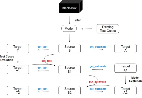
Figure 7 Process structure 20
L I S T O F L I S T I N G S
L I S T O F A B B R E V I AT I O N S
1
I N T R O D U C T I O NSoftware is an essential key in many devices and systems of our society and defines the behavior of many infrastructures of modern life. From mundane appliances like mi-crowaves, mobile phones and cars to more delicate applications such as airplanes and spaceships, software plays an important role. For those more delicate applications, even more than for the mundane ones, a special attention is needed. Many factors affect the engineering of reliable software, such as careful design and sound process management. However, testing is still the primary hardware and software technique used by the industry to evaluate software under development — and it consumes between 30 and 60 percent of the overall development effort (Utting and Legeard, 2007). Usually, testing is ad hoc,
error-prone, and very expensive (Broy et al.,2005). Fortunately, a few basic software testing
concepts can be used to design tests for a large variety of software applications (Ammann and Offutt,2008). The goal of this thesis is to provide an easier and efficient testing
envi-ronment through the use of model-based testing, where the model of the system under test is synchronized with its test cases and the developer is able to evolve the model by either evolving the model itself or its test cases, therefore being bidirectional.
1.1 m o t i vat i o n
Every piece of software, regardless of its goal, needs to be tested — and testing takes a lot of development effort. We aim to make testing easier and more efficient. It is common to find automated test execution as in Vukota Pekovi´c(2010), but model-based testing pushes
the level of automation even further by automating the design, not just the execution of the test cases (Utting and Legeard,2007). In model-based testing, test cases are derived from
a model and not from the source, therefore it can be seen as one form of black-box testing. Frequently, the source code is not available, or the code is too messy, or there is almost no documentation. We can bypass this by using black-box testing. This testing technique observes the behaviour of the system under test. It uses inputs and outputs to build a model of how the system under test reacts in response to an action. The model built by this technique is a good alternative to the source code when used for purposes like testing. It is
1.1. Motivation 2 easier to observe this model instead of the source code. However, not all code is modeled and it takes effort to do so.
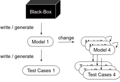
In order to improve software testing, we want to improve the developer’s testing environ-ment. For instance, the developer could be testing manually or creating biased tests from their model, which may cause flaws in the software to be missed. Besides that, they have to keep refining the model until it is a good enough representation of the black-box, i.e., the system under test. At this point, the developer may have repeated this process a lot of times as shown in Figure1. And if the model is not a good representation of the black-box,
it needs to be changed, and new test cases need to be generated in order to check again if this new model is a good enough representation of the black-box. Usually, the way the developer has to change this model is through the submission of new test cases to the black-box. Based on this new output, a new model can be inferred. After the model is inferred, he can start using the model to test the black-box.
Figure 1: Software testing method example.
Our approach lets the developer not only evolve the model by adding new test cases, but also look into the model and change it directly. This way, we provide a way for the developer to choose the more convenient evolution. In addition, the model and test cases are synchronized. Every time one of them is evolved, the other is co-evolved so that there are no inconsistencies.
1.2. Background 3 1.2 b a c k g r o u n d
This thesis makes use of some concepts, methodologies and technologies, that we need to understand before continuing to the main topic.
1.2.1 Model Learning
Machine learning is an application of artificial inteligence that provides systems the ability to automatically learn and improve from experience without being explicitly pro-grammed. The primary aim is to allow computers to learn automatically without human intervention or assistance and adjust actions accordingly. To infer a model for a black-box, it is essential that the learner learns with each pair (input, output), so a machine learning algorithm is needed.
We are routinely learning the behaviour of devices by trial and error. Most of the times, we do not read the manual and start toying with them immediately. Children are especially good at this. They learn how to use a smartphone without anyone telling them and we often get surprised by it. This learning procedure consists in the construction of a mental model or state diagram of the device.
Model inference techniques can either be white box or black box, depending on whether they need access to the source code. This thesis will be based on the black box approach. Not only it is easier to use but it can be applied in situations where the source code is not available.
Through experiments we determine in which global states the device can be and which transitions and outputs occur in response to which inputs. And because specifications are not needed, model learning is an effective method for black-box state machine models of hardware and software components (Vaandrager,2017).
1.2.2 Model-Based Testing
Model-based testing is a testing technique where run time behavior of a system under test is checked against predictions made by a model. In other words, it describes how the system behaves in response to an action. It is a lightweight formal method to validate a system and can be applied for both hardware and software testing.
1.2.3 Black-Box Testing
Many times, the system under test is an executable program and its implementation is unknown or not used , and that’s the reason why it is called a black-box.
1.3. Document Structure 4 Black-box testing is an important software testing technique that executes an applica-tion, or parts of it, without looking into its internal structures or implementation. Then it compares this with the expected result.
1.2.4 Bidirectional Transformations
Bx is a methodology to synchronize two artifacts.
To allow the synchronization of both the test cases and the model, bidirectional tech-niques are needed. They permit a single piece of code to be run in several ways, and will be used to guarantee the conformity between the model and the test cases, automatically done after the test cases or model’s evolution.
1.3 d o c u m e n t s t r u c t u r e
Chapter 1 introduces the problem addressed and essential techniques to solve it. The second chapter digs deeper on each technique and the state of the art. Furthermore, chapter 3 describes the current work on the Haskell prototype. Finally, the fourth and last chapter gives some insight on the work plan and what is expected to be done in the near future.
2
S TAT E O F T H E A R T2.1 m o d e l l e a r n i n g
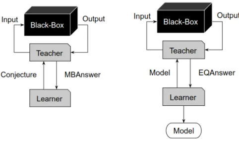
In a membership query, the Learner selects a word and the Teacher gives the answer wether or not this word is accepted by the system under test.
In an equivalence query, the Learner selects a hypothesis automaton and the Teacher answers whether or not this hypothesis is a good representation of the behaviour of the system under test.
2.1.1 L* Algorithm
Worrell’s lecture notes shows that Angluin’s L* algorithm is an exact learning procedure for the class of regular languages. And as said before, the model can be seen as an automa-ton and the inputs as test cases, that are phrases of the language that the automaautoma-ton defines. So, this algorithm can be used to learn this language.
Suppose that the target is a regular language L over an alphabet Σ. It is assumed that Σ is known to the learner. Moreover it is supposed that the learner has access to an oracle (called the teacher) that can answer two types of queries: membership queries and equiva-lence queries. Membership queries answer whether a word chosen by the learner belongs to the target language L or not. Equivalence queries answer if the target language L is the language of the hypothesis automaton created on this procedure. It uses the representa-tion class of deterministic finite automata and is guaranteed to learn the target language submitting queries to the target automaton (i.e., our black-box).
2.2 t e s t c a s e g e n e r at i o n
Test case generation is among the most labour-intensive tasks in software testing. And because software testing is often accounted for more than 50% of total development costs, it is crucial to improve its effectiveness.
2.2. Test Case Generation 6
(a) Membership query. (b) Equivalence query. Figure 2: Membership and equivalence queries.
This thesis only focuses on MBT for generating test cases automatically from a behav-ioral model of a system under test. Therefore, it is the only covered test case generation technique.
Model based testing encompasses three main approaches as referred to in Anand et al.
(2013): axiomatic approaches,Finite State Machine (FSM)approaches, andLabeled Transition
System (LTS)approaches.
The model describes possible input/output sequences on a chosen level of abstraction, and is linked to the implementation by a conformance relation. The test cases are derived from the model by a test selection algorithm, using a testing criteria based on a test hypoth-esis justifying the adequateness of the selection.
Test selection can happen before test execution time by generating test suites, called offline test selection, or in the middle of test execution, called online test selection.
An axiomatic approach will be used for the test cases generation. Axiomatic approaches of MBT are based on logic calculus. Given a conditional equation like p(x) → f(g(x), a) =
h(x), where f , g, and h are functions of the SUT, a is a constant, p a predicate, and x a variable, the objective is to find assignments to x such that the given equality is sufficiently tested. A theorem prover can be used to prove this implication after normalization, but models which use pre- and post- conditions can also be instrumented for MBT using ran-dom input generation instead of theorem proving/constant resolution. An example of this is QuickCheck (Claessen and Hughes,2000) which is the current used tool to generate test
2.3. Deterministic Finite Automaton 7 2.3 d e t e r m i n i s t i c f i n i t e au t o m at o n
A Deterministic Finite Automaton (DFA) is a finite state machine that accepts or rejects strings of symbols and only produces a unique computation of the automaton for each input string.
A deterministic finite automatonM is a 5-tuple,(Q,Σ, δ, q0,F ), consisting of
• a finite set of statesQ
• a finite set of input symbols called the alphabetΣ • a transition function δ :Q ×Σ→ Q
• an initial or start state q0 ∈ Q
• a set of accepted or final statesF ⊆ Q
Let ω= a1a2...anbe a string over the alphabetΣ, where ai ∈ Σ. The automatonMaccepts
the string ω if a sequence of states, r0, r1, ..., rn, exists inQwith the following conditions:
1. r0= q0
2. ri+1=δ(ri, ai+1), for i=0, ..., n−1 3. rn∈ F
The first condition says that the machine starts in the start state q0. The second condition
says that given each character of the string ω, the machine will transition from state to state according to the transition function δ. The last condition says that the machine accepts ω if the last input of ω causes the machine to hault in one of the accepting states. Otherwise, it is said that the automaton rejects the string. The set of strings that M accepts is the language recognized byMand this language is denoted by L(M).
The following DFA M has a binary alphabet and requires the input to contain an even number of 0s. M = (Q,Σ, δ, q0,F )where • Q = {S1, S2} • Σ= {0, 1} • q0 =S1 • F = {S1}
2.4. Bidirectional Transformations 8 • δ is defined by the following state
transition table:
0 1
S1 S2 S1
S2 S1 S2
2.4 b i d i r e c t i o na l t r a n s f o r m at i o n s
Bidirectional Transformations (BXs) provide a way to maintain consistency between two pieces of related information, referred to as the source and the view.
bx :: S o u r c e V i e w
A bidirectional transformation consists of a pair of transformations (get, put), called lens.
get bx :: s - > M a y b e v put bx :: s - > v - > M a y b e s
The core language BiGUL, designed and implemented by Hsiang-Shang Ko and Hu
(2013), is a putback-based bidirectional programming language that allows the programmer
to write only one putback transformation, from which the unique corresponding forward transformation is derived for free. This gives full control over the bidirectional behaviour but there must be no ambiguity. The logic of a putback transformation is more sophisti-cated than that of a forward transformation and does not always give rise to well-behaved bidirectional programs. This calls for more robust language design to support development of well-behaved putback transformations.
Throughout this thesis, we will use BiGUL as a bidirectional programming language. The forward transformation get extracts information from a source to construct an ab-stract view. The source usually has more information than the view, so this transformation discards some information in the process. The backward transformation put updates an old source with a new view, producing an updated source, that is synchronized with this new view. Note that these functions can possibly fail, returning the Nothing constructor. Oth-erwise, the successfully computed view is returned wrapped in the Just constructor. Both this constructors are from the Maybe monad.
These lenses should also be well-behaved by satisfying the following round-tripping laws:
∀ s, v put(s, get s) =s (GetPut) ∀s, v get(put(s, v)) =v (PutGet)
The GetPut law says that if we extract a view from the source and then update this source with the exact same view, nothing should be done because the result is the same source.
2.4. Bidirectional Transformations 9 The PutGet law says that after updating a source with a view, if we try to extract a view from the updated source, we should get back the view used to update it.
BiGUL’s core consists of some primitives and combinators for constructing well-behaved bidirectional transformations, which are introduced below.
2.4.1 Skip
The first primitive is Skip:
S k i p :: ( s - > v ) - > B i G U L s v
The put behaviour of Skip f keeps the source unchanged, provided that the view is com-putable from the source by f. In the get direction, the view is fully computed by applying f to the source.
This primitive is often used with the function const (), therefore the following bx was created.
s k i p 1 :: B i G U L s () s k i p 1 = S k i p ( c o n s t () )
skip1 is used everytime it is needed to keep the source unchanged as long as the view matches unit (). The source and view might need to be rearranged in order for the correct elements to be matched.
2.4.2 Replace
The second primitive is Replace:
R e p l a c e :: B i G U L s s
The Replace primitive completely replaces the source with the view.
2.4.3 Product
When we have a source pair(s1, s2)and a view pair(v1, v2), we can use Prod to combine
two putback transformations.
P r o d :: B i G U L s1 v1 - > B i G U L s2 v2 - > B i G U L ( s1 , s2 ) ( v1 , v2 )
bx1 ‘Prod‘ bx2 is a product of two bidirectional transformations that uses v1to update s1
2.4. Bidirectional Transformations 10 2.4.4 Source/View rearrangement
When the source and view have a different structure, we can rearrange them into the same structure through a λ-expression e.
$ ( r e a r r S [| e :: s1 - > s2 |] ) :: B i G U L s2 v - > B i G U L s1 v $ ( r e a r r V [| e :: v1 - > v2 |] ) :: B i G U L s v2 - > B i G U L s v1
2.4.5 Case
The Case combinator is used for case analysis and has the following structure:
C a s e [ $ ( n o r m a l [| m a i n C o n d :: s - > v - > B o o l |] [| e x i t C o n d :: s - > B o o l |] ) == > ( bx :: B i G U L s v ) , ... , $ ( a d a p t i v e [| m a i n C o n d :: s - > v - > B o o l |] ) == > ( f :: s - > v - > s ) , ... ] :: B i G U L s v
It contains a sequence of cases that can be either normal or adaptive. The conditions are tried in order, to decide which branch we should enter.
2.4.6 Example
Let’s think of a simple bidirectional BiGUL program to calculate the length of a string. Because the string contains more information than its length, it is more suitable to be the source. On the other hand, the length can be seen as an abstract view of the string, from which is extracted some information and the remaining discarded. With this in mind, we arrive intuitively at the following type for our bx:
h e l l o B x :: S t r i n g Int
The forward direction gives us the length of the source. When we change the view to a different length, we can run the backward transformation in order to reflect this change to the source and change the actual string.
2.4. Bidirectional Transformations 11
If the new length is inferior, the result of the backward transformation will be a shorter string, cut from the right to the left.
If the new length is greater, the result of the backward transformation will be a bigger string, to which were added spaces, in the right end, equivalent to the diference between the new and old lengths.
The length is usually represented as an Int, but in this case it can’t be. That is because we need to be able to iterate through the string while keeping track of where we are, i.e., how many characters have we counted to the moment, or how many characters are left to count. The Int type is not good for this because BiGUL only allows the rearrangement of the structure of the type and not its value. For this reason, it will be used the Nat type that represents the natural numbers as successors of other numbers, starting in zero. This type allows us to rearrange 1 as Succ (Zero), which then allows us to keep track of where we are, starting in the number n and ending in Zero.
h e l l o B x :: B i G U L S t r i n g Nat h e l l o B x = C a s e [ $ ( n o r m a l S V [ p | [] |] [ p | Z e r o |] [ p | _ |] ) == > $ ( r e a r r V [| \ Z e r o - > () |] ) s k i p 1
2.4. Bidirectional Transformations 12 , $ ( a d a p t i v e S V [ p | _ |] [ p | Z e r o |] ) == > \ _ _ - > [] , $ ( n o r m a l S V [ p | ( _ : _ ) |] [ p | S u c c _ |] [ p | _ |] ) == > $ ( r e a r r S [| \( s : ss ) - > ( s , ss ) |] ) $ $ ( r e a r r V [| \( S u c c n ) - > (() , n ) |] ) $ s k i p 1 ‘ Prod ‘ h e l l o B x , $ ( a d a p t i v e S V [ p | [] |] [ p | _ |] ) == > \ _ ( S u c c n ) - > " " ] 2.4.7 Usage
Bidirectional transformations can be used to maintain the consistency of several sources of information and to provide an abstract view to easily manipulate data and write them back to their source.
3
B I D I R E C T I O N A L F I N I T E S TAT E M A C H I N E B A S E D T E S T I N GBidirectional finite state machine based testing is a methodology that combines model-based testing and bidirectional transformations in a way that aims to improve the devel-oper’s testing environment. It consists of two main phases:
1. Model inference 2. Evolution
Model inference is the process of reasoning through the use of black-box testing to pro-duce a model of the system under test.
Evolution is when we improve the model by either adding new test cases or by directly modifying the model. An important property of this evolution is that the model is always synchronized with its test cases.
3.1 m o d e l i n f e r e n c e
This phase consists on the application of an algorithm based on the L* Algorithm. A Learner will build a model of the behaviour of the black-box. To do so he will have help of a Teacher that answers two types of questions: membership queries and equivalence queries.
Membership queries check if a word is accepted by the black-box. If the word is accepted the answer is Accept, and if the word is a subset of an accepted word, the answer is Perhaps. This is useful to know if a word that is currently rejected can be accepted in the future. Otherwise the answer is Reject.
- - M B A n s w e r is the r e s u l t of the m e m b e r s h i p q u e r y d a t a M B A n s w e r
= A c c e p t - - | The w o r d is a c c e p t e d by the black - box | R e j e c t - - | The w o r d is r e j e c t e d by the black - box | P e r h a p s - - | The w o r d is a s u b s e t of an a c c e p t e d w o r d d e r i v i n g ( Show , Eq )
3.1. Model Inference 14
Equivalence queries compare the behaviour of the built hypothesis model with the be-haviour of the black-box. It is considered that the hypothesis model is a good representa-tion of the black-box if both answers to a series of membership queries match. Both the hypothesis model and the black-box receive the same generated test suite for the test. If the hypothesis model is indeed a good representation of the black-box, the answer to the equivalence query will be EQUIV. Otherwise, the first failed test case is given as a coun-terexample.
- - E Q A n s w e r is the r e s u l t of the e q u i v a l e n c e q u e r y d a t a E Q A n s w e r sy
= E Q U I V | The h y p o t h e s i s a u t o m a t a is e q u i v a l e n t to the black -box
| CEX [ sy ] - - | C o u n t e r e x a m p l e d e r i v i n g ( Show , Eq )
The Teacher helps the Learner by providing both the previous queries. He is the bridge between the Learner and the black-box.
- - The T e a c h e r a n s w e r s q u e s t i o n s to the L e a r n e r d a t a T e a c h e r st sy = T e a c h e r
{ - - | A s n w e r s w h e t h e r a w o r d is a c c e p t e d by the black - box or not i s M e m b e r :: [ sy ] - > M B A n s w e r ,
- - | A n s w e r s w h e t h e r the h y p o t h e s i s a u t o m a t a is e q u i v a l e n t to the black - box or not
i s E q u i v :: Dfa st sy - > E Q A n s w e r sy }
So far, we have a Learner that asks two types of queries to a Teacher in order to learn the behaviour of a black-box. This is an iterative process. Until the hypothesis model represents the black-box, the Learner keeps improving it. To save the progress made, it is used the following structure: - - S t a t e of the l e a r n i n g a l g o r i t h m d a t a L e a r n e r S t a t e st sy = L e a r n e r S t a t e { - - | L i s t of s t a t e s g e t R :: [ st ] , - - | L i s t of c o u n t e r e x a m p l e s g e t E :: [[ sy ]] ,
3.1. Model Inference 15 - - | N e x t new s t a t e g e t N S :: st , - - | L i s t of p o s s i b l e f i n a l s t a t e s g e t G :: [( st , [ sy ] , [ M B A n s w e r ]) ] , - - | L i s t of p o s s i b l e t r a n s i t i o n s g e t G S :: [( st , sy , [ M B A n s w e r ]) ] }
This data type keeps the state of the learning algorithm. The hypothesis model is a deterministic finite automata built from this structure. Because the types used for states and symbols can vary, they are received as arguments.
In our case study, the states are integers (Int) and the symbols are characters (Char), therefore the structure will be LearnerState Int Char.
This structure is composed of 5 components, and we can use the correspondent get function to retrieve their value:
• getR gives the list of states;
• getE gives the list of counterexamples; • getNS gives the next new state.
• getG gives a list of possible final states; • getGS gives a list of possible transitions.
After the learner state is initialized, the learning procedure begins. In every iteration, we check if the learner state is closed, i.e., if we can’t reach a new state from the ones currently available. If there is a new state we can reach, the learner state is changed to incorporate this new information. Otherwise, a hypothesis model is built from the closed learner state, in order to evaluate if it represents the system under test. This evaluation, as known as equivalence query, is done by submiting a suite of test cases to both the system under test and the model. If both outputs are the same, means that the model behaved in the same way that the system under test did and therefore is a good enough representation. The test suite is generated by QuickCheck (Claessen and Hughes, 2000). If the hypothesis model
does not represent the behaviour of the system under test, a counterexample is used to change the learner state so that we get closer to a better representation. Of course, the most challenging part of this algorithm is the way the learner state is changed to incorporate new changes. And this will also affect the quality of the model.
3.2. Evolution 16 3.2 e v o l u t i o n
The second phase is initiated after a model is built in the first phase. In this phase, the developer will be able to evolve the model and co-evolve the test cases, and vice versa. This is achieved by utilizing bidirectional transformations to synchronize our artifacts.
The artifacts are the model and the test cases. The first thing we must do is choose which one is the source and which one is the view. Keep in mind that the view usually has less information than the source, it is a sort of abstraction. We should be able to obtain the view from the source.
3.2.1 Test Cases Source
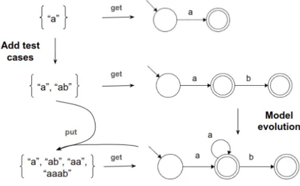
Let’s start by assuming the test cases are the source and the model is the view, like in the next evolution example. From the source{”a”}, we can’t build the unique DFA that accepts that test case, because there are an infinite number of DFAs that accept the test case ”a”. The forward transformation must be deterministic and this one isn’t. However, we can consider the view to be the minimal DFA, and it works, for this case. If we add another test case, we can get the correspondet view just like in the previous one. The problem comes when we start using loops. In the model evolution, the developer added a loop. This change needs to be put back into the source. But we don’t have a source whose unique view is this one. For instance, the test cases in the source{”a”, ”ab”, ”aa”, ”aaab”}are accepted by the target DFA, but we can’t retrieve this view from this source. We don’t know whether there must be a loop or not based on this source. Therefore, this artifact configuration is not possible.
3.2. Evolution 17 3.2.2 Model Source
Now, we can try the other way around by assuming the model is the source and the test cases are the view. From the first DFA, we can get the view{”a”}, as it is the only test case accepted by the source DFA. The source is then evolved to the second DFA. Since it has a loop, we don’t know how many test cases the forward transformation should generate. Like in the previous example, we can restrict the view so that the forward transformation is deterministic. In this case, the number of times a loop is executed can be fixed at one. This way, the view of the second source is {”a”, ”aa”}. However, it is not that simple in the backward transformation. If the developer adds a test case like ”aaa”, we can’t put the changes back to the source. The source already accepts the test case, but it is not generated because of the restriction we added in order to solve the previous problem. Therefore, this artifact configuration is also not possible.
Figure 4: Evolution example with the model as the source and the test cases as the view.
3.2.3 Complex Source
These assymetric lenses do not work because each of the artifacts have information the other does not have. From a set of test cases, it is possible to build more than one DFA.
3.2. Evolution 18 And from one DFA, it is possible to generate more than one set of test cases. To solve this, we can use two assymetric lenses with a common source. The common source stores enough information so that it is possible to retrieve the model and test cases with their correspondent forward transformation. As for the two views, we have the model and the test cases. Both of them can be changed like before to update this complex structure.
The simplest structure to store this information is a pair of both involved views as shown in the next example. With this complex source, both views are unique and there is no ambiguity. For this pair structure, both forward transformations are straight forward. They are just a simple get. When the developer adds test cases, they must be added to the test cases set in the source, and the model must also be changed to accept these new test cases. When the developer evolves the model, it is only needed to check the test cases set in the source for incompatibilities. If there are test cases that are no longer accepted, we can either give an error message or remove them.
Figure 5: Evolution example with two views and a pair structure as the source.
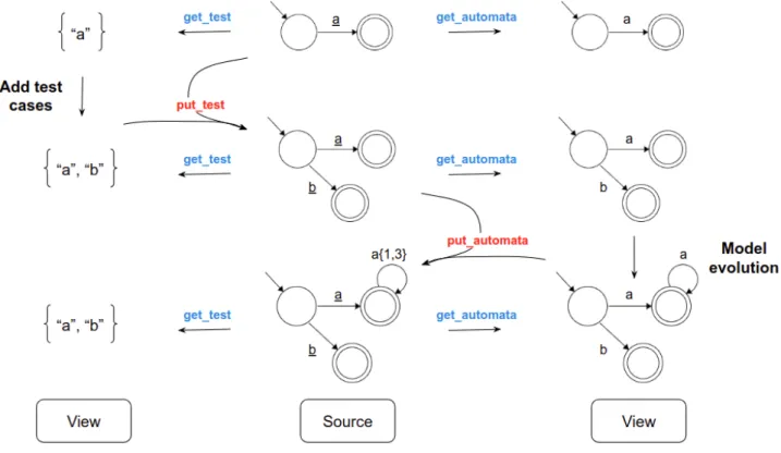
There is also the possibility of using a more complex structure that blends the test cases in the model as annotations. The advantage of mixing the information is that the bidirec-tional language, in our case BiGUL, will guarantee more properties. For instance, with the previous source, to retrieve the test cases, it does not matter how the model is, if it is well built or not. With this source, to retrieve the test cases, we must go throught each
transi-3.3. Overview 19 tion and check the annotations. This way, we know that at least the transitions for those test cases exist. The down side of this type of source is that the problem gets even more complicated.
In the next example, we can see that only the underlined transitions are used to extract the test cases. On the other hand, extracting the model is way easier. It is just needed to remove the annotations. To solve the problem with loops, we can have an annotation that tells us how many times the transition must be repeated. For the transition a1, 3 will be two different test cases, one repeats the transition one time and the other three times. But because this transition is not underlined, those test cases are not generated.
Figure 6: Evolution example with two views and a complex structure as the source.
3.3 ov e r v i e w
With phase 1, the developer can infer an initial model for the black-box. And in phase 2, he is able to improve this model in two different ways. This let’s him choose how the model is evolved and also helps with the consistency between the model and its test cases. The structure of this process can be seen in the next figure.
3.3. Overview 20
4
H O W T O U S E4.1 m o d e l i n f e r e n c e
To infer a model for a black-box, we can use the function lstar, whose type is as follows:
l s t a r :: ( Eq st , Eq sy , Num st , F i n i t e sy , S h o w st , S h o w sy ) = > T e a c h e r st sy - > Dfa st sy
We can call it with by writing lstar teacher. It receives a teacher, who is able to answer membership and equivalence queries. As a result, we get a deterministic finite automata that behaves like the black-box.
For instance, imagine a black-box that behaves like the regular expression ”aa”. It will only accept that word and nothing else, therefore its vocabulary is just the symbol ’a’. Given a teacher, who is able to ask membership and equivalence queries to this black-box, let’s follow the state of the learning algorithm.
It starts by initializing the learning state. The first variable is the list of states, whose initial length is 2. The state 0 is the error state and the state 1 is the initial state. Following it, we have a list with the counterexamples found. Currently, only the empty word is a current example because it is the simplest not accepted word. The next state variable is pretty straight forward. It just keeps track of the number of the next state. Because the last state is the state 1, the next one will be state 2. In the next two lists, it is saved the possible final states and possibles transitions, respectively. For each possible final state, initially it is only the initial state, we have a triple that has the respective state, the word used to reach that state and the answer to a membership query using this word. For the possible transitions, it searches for every possible transition and checks if the current word plus the new symbol is accepted. In this case, from the state 1, it may be possible to go through the symbol ’a’ to another state. If there were more symbols in the vocabulary, more transitions would be considered.
g e t R = [0 ,1]
4.1. Model Inference 22
g e t E = [ " " ] g e t N S = 2
g e t G = [(1 , " " ,[ P e r h a p s ]) ] g e t G S = [(1 , ’ a ’ ,[ P e r h a p s ]) ]
With the learner state initialized, ´ıt checks the list of possible transitions and finds a tran-sition yet to explore. Because it found a possible trantran-sition, it returned NewNext (1,”a”,2). Having found a new possible transition, it switchs to subroutine that handles new transi-tions. The subroutine handleNewNext is responsible for the update of the learner state, adding the required information in order to learn with this new transition.
In the following example, we see that it was adding the new state to the list of states. The next state was incremented to 3. And from the new state (state 2), were created two triples. The first one checks if arriving at the state 2 from the path ”a” results in an accepted state. The second one is a new possible transition, starting form the new state, through the symbol ’a’. And this transition arrived at an accepted state.
g e t R = [0 ,1 ,2] g e t E = [ " " ] g e t N S = 3
g e t G = [(1 , " " ,[ P e r h a p s ]) ,(2 , " a " ,[ P e r h a p s ]) ] g e t G S = [(1 , ’ a ’ ,[ P e r h a p s ]) ,(2 , ’ a ’ ,[ A c c e p t ]) ]
After updating the learner state, it checks again for a new possible transition and founds the first not used transtion, returning NewNext (2,”a”,3). Like before, the subroutine
han-dleNewNextwill update the learner state while taking this new transition in consideration. And we get the following learner state.
g e t R = [0 ,1 ,2 ,3] g e t E = [ " " ] g e t N S = 4
g e t G = [(1 , " " ,[ P e r h a p s ]) ,(2 , " a " ,[ P e r h a p s ]) ,(3 , " aa " ,[ A c c e p t ]) ] g e t G S = [(1 , ’ a ’ ,[ P e r h a p s ]) ,(2 , ’ a ’ ,[ A c c e p t ]) ,(3 , ’ a ’ ,[ R e j e c t ]) ]
At this point, when it tries to search for more possible transitions using symbols of the vocabulary, they are rejected. That means that there are no more possible transitions available and that the next state is the state 0 (error state) by returning HasNext 0.
When it gets to a point where there are no more transitions available, it will check if the learning procedure is complete by asking an equivalence query to the teacher. If the
4.1. Model Inference 23 answer is EQUIV, the learning procedure is complete and the model returned. Otherwise, a counterexample where the model fails is given in order to rectify the learner state. The subroutine handleCex is responsible for it, and is one of the most important just like
han-dleNewNext, because they are responsible for the evolution of the model.
In the end, we get the DFA that represents the behaviour of the black-box. To confirm this, we can check it by writing dfaaccept dfa ”aa”. It will return True and if we use any other word, it will return False.
dfa = Dfa v q s z d e l t a w h e r e v = " a " q = [0 ,1 ,2 ,3] s = 1 z = [3] - - d e l t a :: st - > sy - > st d e l t a 0 ’ a ’ = 0 d e l t a 1 ’ a ’ = 2 d e l t a 2 ’ a ’ = 3 d e l t a 3 ’ a ’ = 0
5
C O N C L U S I O NThis dissertation shows a new methodology that combines model-based testing and bidi-rectional transformations.
In the context of the 2nd call of the NII Internation Internship Program, I was accepted to work at theNational Institute of Informatics (NII)in Japan, under the supervision of Professor Hu. In a recent video conference, Professor Hu showed interest in this subject and proposed the prototype to be written in Bidirectional Generic Update Language (BiGUL), a language designed forBidirectional Transformations (Bx)developed by a research team atNII.
We tried to use a bidirectional language in order to synchronize the model with its test cases. However, the bidirectional language used has many restrictions and writing in it is very hard. Therefore the results weren’t as we expected.
B I B L I O G R A P H Y
Paul Ammann and Jeff Offutt. Introduction to Software Testing. Cambridge University Press, New York, NY, USA, 1 edition, 2008. ISBN 0521880386, 9780521880381.
Saswat Anand, Edmund K. Burke, Tsong Yueh Chen, John Clark, Myra B. Cohen, Wolfgang Grieskamp, Mark Harman, Mary Jean Harrold, and Phil Mcminn. An orchestrated survey of methodologies for automated software test case generation. J. Syst. Softw., 86(8):1978– 2001, August 2013. ISSN 0164-1212. doi: 10.1016/j.jss.2013.02.061. URL http://dx.doi.
org/10.1016/j.jss.2013.02.061.
Manfred Broy, Bengt Jonsson, Joost-Pieter Katoen, Martin Leucker, and Alexander Pretschner. Model-Based Testing of Reactive Systems: Advanced Lectures (Lecture Notes in Computer Science). Springer-Verlag, Berlin, Heidelberg, 2005. ISBN 3540262784.
Koen Claessen and John Hughes. Quickcheck: A lightweight tool for random testing of haskell programs. In Proceedings of the Fifth ACM SIGPLAN International Conference on Functional Programming, ICFP ’00, pages 268–279, New York, NY, USA, 2000. ACM. ISBN 1-58113-202-6. doi: 10.1145/351240.351266. URLhttp://doi.acm.org/10.1145/351240.
351266.
Tao Zan Hsiang-Shang Ko and Zhenjiang Hu. Bigul: A formally verified core language for putback-based bidirectional programming. J. Syst. Softw., 86(8):1978–2001, August 2013. ISSN 0164-1212. doi: 10.1016/j.jss.2013.02.061. URLhttp://dx.doi.org/10.1016/j.jss. 2013.02.061.
Mark Utting and Bruno Legeard. Practical Model-Based Testing: A Tools Approach.
Mor-gan Kaufmann Publishers Inc., San Francisco, CA, USA, 2007. ISBN 0123725011,
9780080466484.
Frits Vaandrager. Model learning. Commun. ACM, 60(2):86–95, January 2017. ISSN 0001-0782. doi: 10.1145/2967606. URLhttp://doi.acm.org/10.1145/2967606.
Ivan Resetar Tarkan Tekcan Vukota Pekovi´c, Nikola Tesli´c. Test management and test ex-ecution system for automated verification of digital television systems. July 2010. URL
https://ieeexplore.ieee.org/abstract/document/5523721.
James Worrell. Exactly learning regular languages using membership and equivalence queries. Department of Computer Science, University of Oxford. Lecture notes.