Master in
Mathematical Finance
Masters Final Work
Internship Report
Practical approach for probability of default
estimation under ifrs
9
B ´arbara Leit˜ao Santos
Master in
Mathematical Finance
Masters Final Work
Internship Report
practical approach for probability of default
estimation under ifrs
9
B ´arbara Leit˜ao Santos
supervisors
:
Dr. ˆangela barros
Prof. jorge lu´is
Abstract
This report is part of the conclusion of the Master degree in Mathematical Finance, as a result of a 6-month internship at EY, in Financial Services – Advisory. Due to a recent financial crisis, credit entities had to deal with uncertainty, being credit risk one of the main concerns. Risk management in this type of entities is crucial to assure financial stability, and therefore, there is always a constant need of improvement. During the financial crisis of 2008, risk management failed its man purpose since risk models reveal insufficient to capture the risk deterioration on exposures and fail to estimate credit losses under a change in the economic cycle. Therefore, IFRS 9 becomes the new standard imposed by IASB, in order to replace IAS 39. This internship was a vector to expand my knowledge concerning impairment models and the new regulatory framework of the International Accounting Standard Board based on IFRS 9 Financial instruments, by studying a general approach on a specific perspective of a Portuguese bank. This report focuses on collective impairment, regarding the choices and validation of the model for the risk parameter PD used by the bank institution in analysis under this new standard.
Keywords: Credit Risk, Expected Credit Losses, IFRS 9, Impairment model, Collective impairment, Observed Default Rate, Probability of Default, 12-month PD, Lifetime PD, Point-in-time, Through-the-cycle, Survival analysis, Forward-looking.
Acknowledgements
Firstly, I would like to thank Ângela Barros, for the time and guidance during the whole internship. To the entire team, for their patience and advice that help me to conclude this project and also to EY for the given opportunity.
To Professor Jorge Luís that accepted to be my supervisor since day one, for his guidance and support throughout the internship.
To my family and friends for all the support and motivation along the years. Specially, to my boyfriend, Pedro Figueiredo, that always believed in me and to my parents and sister, Verónica Santos, that have been on my side during my whole life.
Finally, I thank Leonor Lopes for her support and friendship during this two years of Master and internship.
Abbreviations
BM- Behavioral Maturity
CCF- Credit Conversion Factor
EAD- Exposure at Default
ECL- Expected Credit Losses
EL- Expected Losses
IASB- International Accounting Standards Board
IAS- International Accounting Standards
IFRS- International Financial Reporting Standard
KM- Kaplan-Meier estimator
LGD- Loss Given Default
ODR– Observed Default Rate
PD– Probability of Default
PH- Proportional Hazards
SICR– Significance Increase of Credit Risk
Contents
1 Introduction 1
2 Credit Risk and IFRS 9 3
2.1 Credit Risk . . . 3
2.2 Impact of IFRS 9 Financial Instruments . . . 4
2.3 Impairment Models . . . 5 3 Collective impairment 7 3.1 Segmentation . . . 7 3.2 Risk Parameters . . . 8 4 Probability of Default 9 4.1 Definition of default . . . 9 4.2 PD model . . . 9
4.2.1 Observed Default Rate . . . 10
4.2.2 Smoothing curves . . . 13
5 Review of validation methodologies for PD 19 5.1 Qualitative tests . . . 19 5.2 Quantitative tests . . . 20 5.2.1 Results . . . 25 6 Conclusion 30 References 31 A Calibration 33 B Multicollinearity 36
List of Figures
1 Loss distribution of a credit portfolio . . . 4
2 Stages of ECL model . . . 6
3 Credit cycle adjustments . . . 15
4 Confidence interval in a two tailed test . . . 23
5 SQL code for Pearson’s correlation coefficient . . . 25
6 SQL code for Determination coefficient . . . 26
7 SQL code of Binomial test . . . 27
8 Complete SQL code of Binomial test . . . 33
9 SQL code for minimum critical value with normal distribution . . . 34
10 SQL code for maximum critical value with normal distribution . . . 34
11 SAS code for the linear regressions . . . 36
12 Determination coefficient of Euribor rate . . . 37
13 Determination coefficient of Gross domestic product . . . 37
List of Tables
1 Pearson’s correlation coefficient . . . 26
2 Determination coefficients . . . 27
3 Percentage of accepted periods in Binomial test . . . 27
1
Introduction
The present report is part of the conclusion of the Master degree in Mathematical Finance, as a result of a 6-month internship at EY, in Financial Services – Advisory. During this in-ternship, it was possible to apply concepts learned along the course and perform validation methodologies as well gain some insights about market practices. The main goal was ex-panding my knowledge concerning impairment models and the new regulatory framework of the International Accounting Standard Board based on IFRS 9 Financial instruments, by studying a general approach on a specific perspective of a Portuguese bank.
Financial entities have to deal with uncertainty, being credit risk one of the main risks addressed. As risk management in banks is key to ensure financial stability, there is a constant need of improvement in practices and regulations.
Hence due to 2008’s global financing crisis and certain challenges in understating and applying IAS 39, the International Financial Reporting Standard 9 (IFRS 9) was developed during 5 years to replace and fulfill the main gaps, having become mandatory since the 1st of January 2018 and ensuring a more conservative approach to impairments. As a matter of fact, contrary to IAS 39, based on "incurred loss model", this new Standard recognizes credit loss earlier by eliminating the threshold of recognizing a credit loss only after a credit event occurred, in order to ensure more timely recognition of expected credit losses. Therefore impairment models became more forward-looking by incorporating the future economic conditions through macroeconomic variables. The former variables set a range of the most likely possible macroeconomic scenarios, capturing the likelihood of an event of credit loss occurring.
The three main components of IFRS 9 are the classification and measurement of financial assets and financial liabilities, impairment and hedge accounting. The classification of financial instruments is determined at initial recognition and it can be measured at amortised cost, fair value through profit or loss (FVTPL) or at fair value through other comprehensive income (FVTOCI). Hedging accounting is use by banks to manage exposures resulting from risks which can affect losses. The impairment calculation can be done by an individual or collective analysis. On a collective basis, in order to recognize losses for Expected Credit Losses (ECL), three main risk parameters are required: Probability of Default (PD), Loss Given Default (LGD) and Exposure at Default (EAD).
This report focuses on collective impairment, regarding the choices and analysis of the model for the risk parameter PD used by the bank institution in analysis. In order to bet-ter analyze the mentioned topics, it’s organized in 6 distinct chapbet-ters. The second chapbet-ter “Credit Risk and IFRS 9” provides an overview of the credit risk concept and a summary of the Impact of the IFRS 9 Financial Instruments and the new Impairment model. The fol-lowing chapter “Collective impairment”, presents a general view on how credit portfolio is segmented, in the sense of defining the risk profile. It also approaches the main risk param-eters and its influence in the estimation of ECL. In chapter 4 “Probability of Default”, default concept is explained, which is essential to understand the notion of PD. This chapter also provides a possible approach for PD estimation based on the reality of the bank. Afterwards, in chapter 5 “Review of validation methodologies for PD”, the methodology adopted by the bank is analyzed on a qualitative and quantitative basis. Finally in the last chapter, main conclusions are discussed.
2
Credit Risk and IFRS 9
2.1
Credit Risk
During the financial crisis of 2008, risk management in banks was inefficient by failing its main purpose of preventing a bigger crisis [4]. Therefore, there is a constant need of improvement concerning practices and regulations.
Risk is related to uncertainty that may impact negatively the organization. The most relevant types of risk for banks are usually credit, market, liquidity risk, interest rate risk, currency and operational risk.
Being the focus of this report the impairment model and one of its risk parameters, PD, only credit risk is addressed. Credit risk is defined as «the risk of losses due to borrowers’ default or deterioration of credit standing» and the concept of default risk is «the risk that borrowers fail to comply with their debt obligation» [4]. In this sense, credit losses can lead to declines in the asset fair value of companies occurring a difference between its fair value and the book value, which is reported as an impairment loss.
Banks face losses due to borrowers that fail on their obligations. The losses can either be expected (EL) or unexpected (UL). Based on Basel Committee on Banking Supervision [2], the EL is one of the cost components of doing business, impacting on credit pricing and provisioning. The UL are extreme losses, above expected losses, stemming from events that occur only under many unexpected circumstances, which should be 99,9% covered by capital. Therefore, banks need to hold capital in order to ensure their solvency if they face these extreme events [2]. Accordingly, from an economic point of view, capital requirements
must correspond to a very high significance level for the losses distribution. A common methodology used to calculate these extreme losses is the Value-at-risk, for a confidence level of 99.9% and a 12-month time horizon.
Figure 1: Loss distribution of a credit portfolio
When UL covered by capital are computed under Basel requirements, provisions for EL are calculated under IFRS 9 Financial Instruments, which became the new standard in 2018, after being published by IASB on 24 July 2014, replacing the former IAS39 Financial Instruments: Recognition and Measurement.
2.2
Impact of IFRS 9 Financial Instruments
IFRS 9 is a response to the financial crisis of 2008, in particular to the G20 initiatives, in order to impose impairment models ensuring more timely recognition of expected credit losses, addressing weakness of IAS 39 based on an “incurred loss model” [12].
These new rules impose higher levels of impairment since the early stages of deterioration in loans quality, as Lifetime PDs are demanded to calculate provisions whenever impairment signs are triggered. Therefore, IFRS 9 implied a higher level of cyclicality in impairment
models through point-in-time models, in contradiction with capital requirement rules that are based on a through-the-cycle perspective.
This standard imposes three main phases of IASB’s project to replace IAS 39 such as classification and measurement, impairment and hedging accounting [12].
2.3
Impairment Models
The impairment models imposed by IFRS 9 are based on a single forward-looking expected credit loss (ECL) model applied to all financial instruments [12]. According to IFRS standard 9, paragraph B5.5.17, «An entity shall measure expected credit losses of a financial instrument in a way that reflects: (a) an unbiased and probability-weighted amount that is determined by evaluating a range of possible outcomes; (b) the time value of money; and (c) reasonable and supportable information that is available without undue cost or effort at the reporting date about past events, current conditions and forecasts of future economic conditions» [13].
Entities have to recognize the ECL at all times, so the loss allowance must be established since its origination throughout the life of the financial instrument. The approach in this recognition of loss allowance can be either 12-month, which «result from default events on a financial instruments that are possible within 12 months after the reporting date» or Lifetime ECL that «result from all possible default events over the expected life of a financial instrument» [13].
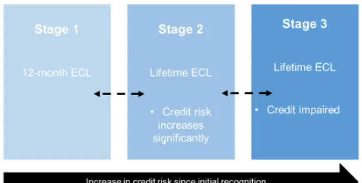
The loss allowance depends on the evidence of significant deterioration in credit risk since initial recognition. Three stages are considered according to the significance of credit deterioration:
• Stage 1 - no significant credit risk deterioration, 12-month ECLs are recognized;
• Stage 2 - significant increase of the credit risk from financial instrument origination or purchase, Lifetime ECLs are recognized;
• Stage 3 - credit-impaired, Lifetime ECLs are recognized.
Figure 2: Stages of ECL model
Based on the figure 2, stage 3 represents obligations that confirm a high deterioration in credit quality. The significant increase of credit risk (SICR) since origination is based on triggers such as an obligation that is 30 days past due (stage 2). Hence, obligations that have in fact defaulted are in stage 3, being one of the triggers the obligations that are 90 days past due [11]. SICR can be assessed on an individual or collective basis, being analyzed in this report the impairment model on a collective basis.
3
Collective impairment
3.1
Segmentation
The collective basis comes from the need of grouping financial instruments, when individ-ual basis is unable to capture the changes in credit risk. Therefore, collective impairment defines the risk profile of each obligation, being assessed together in accordance with credit portfolio segments [11]. Portfolio segmentation is based on shared credit risk characteristics, concerning historical and forward-looking information, such as:
• Collateral type; • Collateral value; • Credit risk rating; • Date of origination; • Instrument type; • Term to maturity; • Type of industry; • Geographical area.
Based on these the obligations are aggregate in homogeneous risk segments, estimating risk parameters according to these. Moreover, IFRS 9 allows these segments to be amended, which implies processes to reassess the similarity of credit risk characteristics over time, in order to obtain a better performed model.
3.2
Risk Parameters
On a collective basis, ECL shall be recognized considering comprehensive credit risk infor-mation such as past and forward-looking macroeconomic inforinfor-mation [11]. The standard does not define a specific procedure to estimate ECLs, hence a general approach for credit losses are based on the following risks parameters:
• Probability of Default (PD): likelihood of borrower won’t accomplish its debt obligation over a certain time;
• Loss Given Default (LGD): percentage of exposure that is expected to be lost by the lender if a default event occurs;
• Exposure ate Default (EAD): estimating outstanding exposure at default time.
A general approach for ECL calculation based on these parameters is given by:
ECL=
N
∑︁
i=1
PD × LGD × EAD (1)
where N is the number of obligations in the portfolio. PD can either be 12-month (stage 1) or Lifetime (stage 2), being excluded from the calculation the obligations that are in stage 3, since are already in default (e.g. PD equal to 1 being ECL = LGD × EAD ). LGD is the expected exposure lost if default occurs and EAD is given by the sum between on-balance sheet exposure and the off-balance sheet exposure that have been converted into credit. Nonetheless, there are other methods to calculate ECL such as the generalised form of the challenger model given by ECB Banking Supervision [9].
4
Probability of Default
4.1
Definition of default
Default can have different meanings according to each institution. IFRS 9 only mentions a «rebuttable presumption that default does not occur later than when a financial asset is 90 days past due» [13], being applied the same definition of default to all financial instrument except for entities with objective information proving the contrary.
4.2
PD model
In the literature, credit risk models integrate one of two classes: structural models and reduced form models (intensity models) [7]. Structural models estimate risk parameters based on debtor structural characteristics, such as assets and liabilities. These models assume default whenever the market value is lower than the value of debt issued. On the other hand, intensity models quantify the probability of default as a function of exogenous variables to the issuer.
Many banks have adapted their Internal rating-based Basel II (UL) for IFRS 9 purposes (EL) [15]. The bank in analysis estimates PD through an intensity model, adjusting PD through-the-cycle to a point-in-time, in order to reflect the recent economic environment.
The PD modelling is divided in three main phases, namely: estimation of observed default rate (chapter 4.2.1), smoothing method (chapter4.2.2) and the forward-looking adjustment method (chapter 4.2.3).
4.2.1 Observed Default Rate
Regarding the default rate estimation, the bank in analysis adopts a Survival analysis. This is a statistical methodology for data analysis where the goal is to model the time until an event of interest occurs [14], which in this case is default.
A particularity of the Survival analysis is the fact of having censored data. Censoring occurs when the exactly default time is unknown. The reasons behind this can be the fact that the operation continuous on the portfolio after the end of the analysis or left it during the analysis period, making it impossible to know the time of default. Therefore, a time horizon is defined for the analysis, being only consider the events occurred in this time interval.
There are two main terms considered in the Survival analysis: the survival function S(t), and the hazard function h(t). The survival function is the probability of a random variable T exceeding a fixed time t,
S(t)= P(T > t) = 1 − P(T ≤ t). (2)
The hazard function is the instantaneous probability for an event to occur, given survival up to time t, h(t)= lim ∆t→0 P(t ≤ T ≤ t+ ∆t|T > t) ∆t (3) Being, f (t)= lim ∆t→0 P(t ≤ T ≤ t+ ∆t) ∆t (4)
and the hazard function also equivalent to
h(t)= f (t)
s(t). (5)
Based on this, there are different types of survival models: non-parametric and parametric models. The Kaplan-Meier (KM) estimator is a common non-parametric model that considers both censored and not censored data. The general KM formula for survival probability until tj is given by, S(tj)= S(tj−1) × P(T> tj|T ≥ tj)= j ∏︁ i=1 P(T> ti|T ≥ ti) (6) Where, S(tj−1)= j−1 ∏︁ i=1 P(T> ti|T ≥ ti) (7) and P(T> ti|T ≥ ti)= 1 −
number of events at time ti
number of items that survived until ti− 1
(8)
As already described, PD is the likelihood of a default occurring in a time horizon that can be either Lifetime or 12-month, depending on the stage of the obligation, in line with ECL estimation. Based on the Survival analysis and Kaplan-Meier, the bank in analysis follows two approaches to estimate Lifetime ODR and 12-month ODR: not correcting for
The estimation of Lifetime ODR is calculated based on a not correcting for censorship approach, given by:
ODRLi f etime =
number of defaults at time t
number of operations that survived until t − 1 (9)
Corresponding to P(T ≤ t|T < ti), which is equivalent to 1 − P(T > ti|T ≥ ti), being the
probability of default occurring until a fixed time t given the ones that survived until t-1 (Formula 2 and 8).
The 12-month ODR is calculated based on cumulative survival rate (SR), which is the product of marginal ODRs. Being estimated according to a correcting for censorship ap-proach that is defined as:
ODR12−month = 1 − SRcumulative. (10)
Where SRcumulative = t−1+12 ∏︁ i=t (1 − ODRi) (11)
being the product of all elements that estimate the probability for a time horizon of 12 months, which corresponds to the survival probability∏︀j−1+12
i=1 P(T> ti|T ≥ ti). Hence, ODR12−month = 1 − t−1+12 ∏︁ i=t (1 − ODRi) (12)
where,
ODRi = ODRmarginal =
number of defaults at time i
number of operations that survived until time i − 1. (13)
4.2.2 Smoothing curves
In order to estimate ECL, the ODR curves need to be smoothed with the purpose of shaping the term structure of the TTC PD, to afterwards capturing the recent economic cycle (PIT PD).
The basis of smoothing arises from «the notion of functions having similar values for “close” observations» [20]. In this sense, smoothing methods allows to capture significant patterns and remove noise from data.
There are many possible methods for smoothing curves. The bank in analysis adopts a three factor base model of Nelson-Siegel (1987), taking into consideration the similarities among interest rates and default rates (ODR). This method is usually used by banks with the purpose of fitting the term structure of interest rates [18], explaining the relationship between interest rate and time to maturity, where the spot rate curve can be obtain by:
yt(τ) = β1+ β2 1 − e−λτ τ λ + β3 [︃ 1 − e−τ λ τ λ −e−λτ ]︃ . (14)
Beingβ1,β2andβ3the three parameters of the model with a constantλ. β1is the long-term
curvature. Theλ is the decay parameter that influences the speed of convergence.
On the one hand, this model can approximate parsimoniously the yield curve with only three parameters, being flexible to capture shapes typically observed in yield curves[18]. On the other hand, it’s not capable of capture all the shapes that the term structure assumes.
Based on this, the bank makes an adaptation of this three-factor model, where the Nelson Siegel fits the PD term structure, being the relationship between the value of ODR and time to maturity.
4.2.3 Forward-looking adjustment
Based on European Banking Authority (2017) paragraph 4.2.6 - Principle 6, «credit institu-tions should use their experienced credit judgment to thoroughly incorporate the expected impact of all reasonable and supportable forward-looking information, including macroeco-nomic factors, on its estimate of ECL» [8].
In this sense, PD has to be estimated according to “point-in-time” (PIT) measures, which tend to adjust quickly to a changing economic environment [2]. PD must be adjusted to incor-porate current credit cycle conditions and assess risk at a given point-in-time, representing the recent economic conditions [17].
On the other hand, when PD estimation is based on “through-the-cycle” (TTC) adjust-ment, it reflects the long-term average of ODR. Therefore, it will not present significant changes during credit cycle, reacting more slowly to changes in macroeconomic conditions over time.
Figure 3: Credit cycle adjustments
The forward-looking adjustment request the incorporation of the most likely multiple possible macroeconomic scenarios. These range of scenarios have to capture the likelihood of an event of credit loss to occur. A possible forward-looking adjustment, is to calculate the PD PIT conditionally for each scenario, being weighted by each probability [15], as following:
PDsi = PD(Z = Xzsi%) (15)
where PDsi is the probability of default for each possible macroeconomic scenario i. Z
is the macroeconomic variable that influences the credit environment and PD(Z = X%) is the probability of default assessment of the facility conditional on a Z growth rate of XZSi% which is than weighted by YSi % chance of this happens.
In accordance with IFRS standard 9, paragraph B5.5.42, there is no evidence of a manda-tory number of macroeconomic scenarios to be used in impairment models [13]. Accordingly, the bank chooses to follow the approach described above with three possible macroeconomic scenarios such as:
• S1 – the baseline scenario, which reflects a probability of YS1% that corresponds to the
current macroeconomic environment;
• S2 – the upside scenario, which attaches a probability of YS2% that the outcome is
better;
• S3 – the downside scenario, which has a probability of YS3% that the outcome is worse;
Concerning the macroeconomic variables, the bank in analysis characterizes it’s credit environment by the following variables: Euribor rate (EURB), gross domestic product (GDP) and 10-year treasury yield (TY10). Being that, the PD under the current forecast of the credit environment (CFCE) is given by three possible scenarios, weighted according to the corresponding probability YSi% [15].
E[PD|underCFCE]= PDS1× 50%+ PDS2× 35%+ PDS3× 15% (16)
where,
PDSi = PD(EURB = XEURBsi%)+ PD(GDP = XGDPsi%)+ PD(Z = XTY10si%). (17)
Being 50%, 35% and 15% the probability of each scenario 1, 2 and 3, respectively. Conse-quently, although it might suggests, the PD for each scenario does not have to be represented by a linear regression. The incorporation of the macroeconomic variables for this method is performed by a Cox regression.
Cox proportional hazards model
The forward-looking adjustment requests a mathematical model to estimate the conditional probability of default under macroeconomic variables. A popular model used for analyzing survival data is the Cox proportional hazards (PH) model [14].
The Cox PH model is defined based on the hazard function,
h(t, X) = h0(t)e ∑︀n
i=1βiXi (18)
where X = (X1, X2, ..., Xn) is the set of explanatory variables, h0(t) is the baseline hazard
function with X = 0, depending only on time t. β is the regression coefficient for each variable X.
Therefore h0(t) corresponds to the nonparametric part andβiXi to the parametric part of
the model. In this way and in accordance with the fact that h0(t) is an unspecified function,
the Cox PH is a semiparametric model which is a reason why is so popular.
The proportional hazard assumption states that «the hazard for one individual is pro-portional to the hazard for any other individual, where the propro-portionality constant is independent of time» [14]. The hazard ratio compares two different specifications of the explanatory variables X* and X, HR= h(t, X * ) h(t, X) = e ∑︀n i=1βi(X*i−Xi). (19) where X* = (X* 1, X * 2, ..., X *
same explanatory variable.
Based on Miu P. and Ozdemir B. (2017) and according to Cox PH, the hazard function h(t, X), is the corresponding conditional PD PIT under three macroeconomic variables and the baseline hazard, h0(t), is the corresponding PD TTC [15]. The Cox PH model can then be
given by,
PD(t, X) = PD0(t)e ∑︀n=3
i=1 βi(X*i(τ)−Xi). (20)
Where t represents the time on which the obligations are at default and τ corresponds to the current period. X = (X1, X2, X3) are the three macroeconomic variables, being X1 =
EURB, X2 = GDP and X3 = TY10. PD0(t) is the PD TTC (12-month PD or Lifetime PD)
that suffers a macroeconomic shock, e∑︀n=3
i=1 βi(X*i(τ)−Xi) called hazard ratio. X*
i is the value of
macroeconomic variable at timeτ and Xi is the mean value according to the historical time
horizon. The difference between these two explanatory variables change according to each macroeconomic scenario, representing the growth rate. For example, there is a proportional inverse relationship between GDP and PD, having a negative coefficient β. Therefore, a positive growth rate of GDP will reflect a lower shock, decreasing the value of PD. Hence, for each macroeconomic scenario there is a different percentage of weight associated to each variable.
5
Review of validation methodologies for PD
Validation as a part of the governance model is a responsibility of the bank, even when it is carried out by an independent entity, which focus on conforming and understanding the complexity of the model [19]. Within the scope of an external audit, EY performed an independent review of the impairment model on a collective basis, analyzing validation methodologies and corresponding outcomes in both quantitative and qualitative perspec-tives [3]. These are done based on expert judgment and also on the IFRS 9 and EBA – Guidelines on PD estimation, LGD estimation and treatment of default exposures [8]. Being the practical approach for the key risk parameter, Probability of default, the focus of this analysis.
5.1
Qualitative tests
In a qualitative perspective, it’s crucial to analyze the consistency of the input data and understand the relevance and validity of the rationale behind the processes associated to the PD estimation.
Concerning the consistency of input data, the historical period and its representativeness, such as sample size, needs to be analyzed. According to EBA Guidelines, paragraph 82, «for the purpose of determining the historical observation period (...) additional observations to the most recent 5 years (...) should be considered relevant when these observations are required in order for the historical observation period to reflect the likely range of variability of default rates of that type of exposures» [8].
should be consistent with inputs to other relevant estimates». Hence, information has to be framed according to the same historical period. Also, the evolution between explanatory variables must be consistent in an economic perspective. For example, as GDP increases, the unemployment rate should decrease [8].
Regarding the validity and relevance of PD model assumptions, according to IFRS 9 paragraph 5.5.5 5, «credit risk on a financial instrument has not increased significantly since initial recognition, an entity shall measure the loss allowance for that financial instrument at an amount equal to 12-month expected credit losses». For this reason, an analysis needs to be done in order to confirm the correct incorporation of PD into ECL estimation for stages 1 (12-month PD) and 2 (Lifetime PD) [13].
Furthermore, the mathematical model used to compute the forward-looking adjustment has to be analyzed in accordance with EBA Guidelines paragraph 33, «include criteria to duly consider the impact of forward-looking information, including macroeconomic factors. (. . . ) Economic factors considered (such as unemployment rates or occupancy rates) should be relevant to the assessment and, depending on the circumstances, this may be at the international, national, regional or local level». In this sense, the adequacy of Cox PH model and its macroeconomic variables are study in a conceptual perspective, analyzing the underlying economic rational [8].
5.2
Quantitative tests
In a quantitative perspective, the respective outcomes and inputs of the PD model are analyzed through performance metrics, calibration and multicollinearity analysis [19].
Performance analysis
Firstly, in order to analyze the performance of the smoothing method, tests such as Pearson’s correlation coefficient and Determination coefficient are performed.
The Pearson’s correlation coefficient can be defined as:
r= n ∑︁ i=1 (︃ ODRi−ODR σODR )︃(︃ PDi−PD sPD )︃ (21)
where n is the number of observations in a time horizon,σODRand sPDare the standards
deviations of ODR and the fitted PD, respectively. The ODR is the average of variable ODR and PD is the corresponding average of fitted PD. The value r can take values between -1 and 1, being 1 a positive correlation where the two variables are identical, 0 when there is no correlation and -1 when the two variables are the opposite [6].
The Determination coefficient tests also the performance of the method as well as it fit-ness. This statistic explains the impact of variability in one variable through the relationship to another, being defined as:
R2 = 1 − SSresidual SStotal (22) where SSresidual= n ∑︁ i=1 (PDi−ODRi)2 (23)
and SStotal = n ∑︁ i=1 (ODRi−ODRi)2 (24)
The SSresidualcorresponds to the variation in PD that it’s not explained by the smoothing
method. While the SStotal measures the total amount of variability in PD. Therefore, this
coefficient measures the variation of PD explained by the method in analysis. This coefficient can take values between 0 and 1, where 1 corresponds to a perfect fitness of the method [1].
Calibration
The Binomial test is performed in order to analyze the quality of the model calibration, comparing the estimated PD with the observed default rate [19]. Assuming the following two hypothesis:
• Null hypothesis (H0): the estimated PD is equivalent to the observed default rate; • Alternative hypothesis (H1): the estimated PD and observed default rate are distinct.
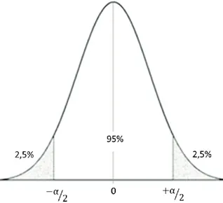
Since this is a bilateral test, the null hypothesis is not rejected if the number of defaults is between two critical values k*
, minimum and maximum, assuming a confidence level q of 95% [3]. These critical values are defined by the cumulative binomial distribution:
PR(k ≤ i)= n ∑︁ i=k (︃n i )︃ i(1 − p)n−i (25)
default and p is the estimated probability of default in a one period.
Hence, based on the binomial distribution, the critical values k*
are given by the two extreme portions of the distribution which leads to rejection (Figure 4).
Figure 4: Confidence interval in a two tailed test
The minimum critical value corresponds to the left tailed, (1 − q)/2, considering an alternative hypothesis where PD is lower than the observed default rate. While the maximum critical value corresponds to the right tailed, 1 − (1 − q)/2, where the PD is higher than the observed default rate.
k* = min{︁k : n ∑︁ i=k (︃n i )︃ i(1 − p)n−i≤ 1 − q 2 }︁ (26) k*= max{︁k : n ∑︁ i=k (︃n i )︃ i(1 − p)n−i ≥ 1 − 1 − q 2 }︁ (27)
[19], as following:
k* = φ−1(q)√︀np(1 − p)+ np (28)
whereφ−1is the inverse of cumulative standard normal distribution.
This approximation is performed in order to conform the results obtained by the cumu-lative binomial distribution (Appendix A).
Multicollinearity analysis
Furthermore, the Variance inflation factor (VIF) is calculated to analyze the need of diminish the multicollinearity of the independent variables incorporated in forward-looking adjust-ment. The VIF is used to analyze the collinearity, eliminating the variables that inflate the variance on others [16]. This measures is defined in terms of R2
i, as following: VIF= 1 1 − R2 i (29) where 1 − R2
i corresponds to the tolerance level, which is the variation of the ith
inde-pendent variable that is not explained by the model. A VIF of 10 or more (less than 0,1 of tolerance level) indicates a problem of multicollinearity, therefore these variables must be eliminated from the model.
5.2.1 Results
The quantitative tests were performed with SAS Software, being analyzed eight PD Lifetime curves (PD-01, PD-02, PD-03, PD-04, PD-05, PD-06, PD-07, and PD-08) of mortgage loans. The results and analysis of the tests mentioned are below.
Performance analysis
The Pearson’s correlation coefficient is performed using SQL within SAS Software, even though it’s also possible to use a SAS statistical procedure namely the PROC CORR statement. The coefficient computation is divided in two parts. Firstly, it’s defined the numerator, covariance, as a and the multiplication between variances as b (Formula 21). Afterwards, the Pearson coefficient is calculated as below:
Figure 5: SQL code for Pearson’s correlation coefficient
Based on the results below, all coefficients are positive and greater than 0,9, existing only one curve (PD-03) lower than 0,9. Consequently, all curves are highly to moderately
correlated, and the smoothing model for these curves is adequate.
Table 1: Pearson’s correlation coefficient
PD curve PD-01 PD-02 PD-03 PD-04 PD-05 PD-06 PD-07 PD-08 Coefficient 0,977 0,998 0,776 0,987 0,955 0,992 0,982 0,997
The Determination coefficient is also computed using SQL, being a firstly computed as the residual sum of squares and b as the total sum of squares (Formula 22). Subsequently, the coefficient is computed as R2.
Figure 6: SQL code for Determination coefficient
Analyzing both coefficients results, the values of R2 are lower than the ones obtained for Pearson’s correlation. Since PD-03 has a determination coefficient lower than 0,7 and a Pearson’s correlation around 0,7, the smooth model for this curve should be adjusted in order to obtain an better performance [1][6]. The remaining curves, despite the differences between coefficients, demonstrate a good performance of the smoothing model.
Table 2: Determination coefficients
PD curve PD-01 PD-02 PD-03 PD-04 PD-05 PD-06 PD-07 PD-08 Coefficient 0,876 0,975 0,446 0,916 0,853 0,944 0,908 0,972
Calibration
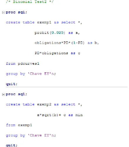
The Binomial test is performed by SQL, being calculated both critical values k*as a function of quantile which is the inverse of the cumulative binomial distribution. The minimum value, defined by a probability of (1 − q)/2 equals to 0,025 and the maximum by a probability of 1 − (1 − q)/2 that equals 0,975.
Figure 7: SQL code of Binomial test
The results obtained can be seen in the Appendix A. The table below represents the percentage of periods in which the number of defaults were between these two critical values, minimum and maximum. Analyzing the following table, it is possible to conclude that all curves are well calibrated since the percentage of acceptance is all greater than 70%.
Table 3: Percentage of accepted periods in Binomial test
PD curve PD-01 PD-02 PD-04 PD-05 PD-06 PD-07 PD-08 Coefficient 94% 88% 93% 90% 87% 82% 78%
Multicollinearity analysis
Based on the previous description of the VIF, a linear regression of the macroeconomic variables is estimated in SAS through a PROC REG statement (Appendix B). Firstly, in order to compute the determination coefficient with respect to the Euribor rate (EURB), a linear regression is computed:
EURB= β0+ β2GDP+ β3TY10 (30)
where EURB is the independent variable and the gross domestic product (GDP) and 10-year treasury yield (TY10) are the dependent ones.
Afterwards, based on this determination coefficient, the VIF of EURB is computed. This procedure is repeated for the gross domestic product and 10-year treasury yield, respectively.
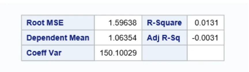
Given the output of SAS (see Appendix B), the VIF of EURB, GDP and TY10 are the following: VIFEURB = 1 1 − R2 EURB = 1 − 0, 01311 = 1, 01327 (31) VIFGDP = 1 1 − R2 GDP = 1 1 − 0, 4011 = 1, 66973 (32) VIFTY10= 1 1 − R2 TY10 = 1 1 − 0, 3974 = 1, 65948 (33)
Therefore, as all values of VIF are between 1 and 2, one can conclude that the collinearity of the variables is low, as the tolerance level is high. Moreover, these variables don’t inflate the variance of the others, being accepted in the forward-looking adjustment.
6
Conclusion
The goal of this project was to analyze a real approach for modeling PD in the calculation of Expected Credit Loss, under the new standard IFRS 9 Financial Instruments.
Banks had to adjust their models in order to fulfill this standard. Based on it, the method-ology was analyzed conceptually and analytically through qualitative and quantitative tests, respectively. The performance and calibration of the model were analyzed by using Pear-son’s correlation, Determination coefficient and Binomial test. The results suggest that this approach estimates well the risk parameter, since the coefficients are greater than the thresh-old of 0,7 and the percentage of the periods accepted is also greater than 70%. Although one of the curves needs to be adjusted, since it presents a determination coefficient of 0,45. Furthermore, the results from multicollinearity suggest that the macroeconomic variables don’t inflate the variance on others, presenting a tolerance level close to 1 which indicates that the variation in one of the variables is not explained by others.
For further research, it would be interesting to develop a Duration method in SAS, which is a Rating Transition Matrix model based on Markov chain assumptions. Comparing it with the approach analyzed in this project, over several validation methods.
To conclude, this project contributes with a better understanding of the impact of IFRS 9 on the collective impairment model of a real bank, especially on the risk parameter PD, and also on the multiple validation methods that can be performed.
References
[1] Asuero, A.G., Sayago, A. and González, A.G. (2006). The Correlation Coefficient: An Overview. Taylor and Francis Group
[2] Basel committee on Banking Supervision. (2005). An Explanatory Note on the Basel II IRB Risk Weight Functions. BCBS, Basel.
[3] Basel Committee on Banking Supervision. (2005). Working Paper No.14, Studies on Vali-dation of Internal Rating Systems. Bank for International Settlements.
[4] Bessis, J. (2015). Risk Management in Banking. Wiley.
[5] Beygi, S., Makarov, U., Zhao, J. and Dwyer D. (2018). Modeling Methodology, Features of a Lifetime PD Model: Evidence from Public, Private and Rated Firms. Moody’s Analytics. [6] Brozek, K. and Kogut, J. (2016). Analysis of Pearson’s linear correlation coefficient with the use
of numerical examples.
[7] Chatterjee, S. (2015). Centre for Central Banking Studies. Modelling credit risk. Bank of England.
[8] European Banking Authority. (2017). Guidelines on PD estimation, LGD estimation and the treatment of defaulted exposures.
[9] European Central Bank. (2018). Asset Quality Review. Banking Supervision
[10] Engelmann, B. and Rauhmeier, R. (2011). The Basel II Risk Parameters, Estimation, Validation, Stress Testing – with Applications to Loan Risk Management. Second edition, Springer.
[12] IFRS Foundation. (2014). IFRS 9 Financial Instruments - Project Summary. IASB. [13] IFRS Foundation. (2014). IFRS Standard 9 Financial Instruments. IASB.
[14] Kleinbaum, D.G. and Klein, M. (2005). Survival Analysis, A Self-Learning Text. Second Edition, Springer, New York.
[15] Miu, P. and Ozdemir, B. (2017). Adapting the Basel II advanced internal-ratings-based models for International Financial Reporting Standard 9. Journal of Credit Risk.
[16] O’brien, R. (2007). A Caution regarding rules of thumb for variance inflation factors. Quality & Quantity. Springer.
[17] Parmani, D. (2017). Whitepaper, Forward-looking Perspective on Impairments using Expected Credit Loss. Moody’s Analytics.
[18] Pooter, M. D. (2007). Examining the Nelson-Siegel Class of Term Structure Models. Tinbergen Institute, EconStor.
[19] Scandizzo, S. (2016). The Validation of Risk Models, A Handbook for Practitioners.
[20] Schimek, M. G. (2000). Smoothing and Regression: approaches, computation and application. John Wiley & Sons.
Appendix
A
Calibration
The information below includes all the complementary code and results, regarding the two approaches for the Binomial test, through a cumulative binomial distribution and a normal distribution.
Figure 9: SQL code for minimum critical value with normal distribution
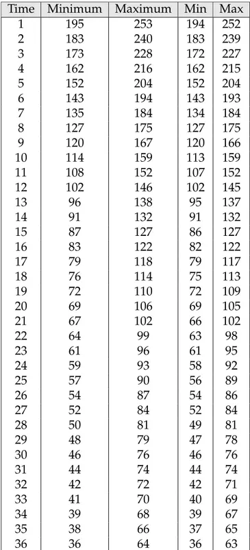
The following PD-01 curve results, regarding the two approaches, belong to a time horizon of three years.
Table 4: Results of Binomial tests
Time Minimum Maximum Min Max 1 195 253 194 252 2 183 240 183 239 3 173 228 172 227 4 162 216 162 215 5 152 204 152 204 6 143 194 143 193 7 135 184 134 184 8 127 175 127 175 9 120 167 120 166 10 114 159 113 159 11 108 152 107 152 12 102 146 102 145 13 96 138 95 137 14 91 132 91 132 15 87 127 86 127 16 83 122 82 122 17 79 118 79 117 18 76 114 75 113 19 72 110 72 109 20 69 106 69 105 21 67 102 66 102 22 64 99 63 98 23 61 96 61 95 24 59 93 58 92 25 57 90 56 89 26 54 87 54 86 27 52 84 52 84 28 50 81 49 81 29 48 79 47 78 30 46 76 46 76 31 44 74 44 74 32 42 72 42 71 33 41 70 40 69 34 39 68 39 67 35 38 66 37 65 36 36 64 36 63
B
Multicollinearity
The information supported includes all the code and results from SAS Software, regarding the multicollinearity test - Variance Inflation Factor.
Figure 12: Determination coefficient of Euribor rate
Figure 13: Determination coefficient of Gross domestic product