USING CREDIT SCORING METHOD FOR PROBABILITY OF NON-FINANCIAL COMPANIES DEFAULT ESTIMATION AT INDUSTRY LEVEL

(1)

USING CREDIT SCORING METHOD FOR PROBABILITY

OF NON-FINANCIAL COMPANIES DEFAULT

ESTIMATION AT INDUSTRY LEVEL

Prof. Ioan TRENCA, PhD

Assist. Annamária BENYOVSZKI, PhD Student „Babeş-Bolyai” University, Cluj-Napoca

Introduction

The credit scoring models are multivariate models which use the main economic and financial indicators of a company as input, attributing a weight to each of them, that reflects its relative importance in forecasting default. The result is an index expressed as a numerical score, which indirectly measures the borrower’s probability of default (Resti, A. & Sironi, A., 2007:287). These models were applied with success in credit institutions.

Despite the techniques underlying credit scoring models were devised in the’30s, in the articles by Fischer, R. A. (1936) and Durand, D. (1941), these models were developed further in the ’60s in papers by Beaver, W. (1967) and Altman, E. I. (1968). Beaver, W. (1967) using a sample of 158 companies (79 non-defaulted companies, 79 defaulted companies) analyzed the predictive power of 14 indicators to classify companies in two categories (defaulted and non-defaulted), using the univariate discriminant analysis. Altman, E. I. (1968) developed a multiple discriminant analysis method on a sample of 66 companies (33 non-defaulted and 33 non-defaulted companies) with 5 financial ratios for the 1946-1965 period.

The multiple discriminant analysis have been used by many other authors to estimate the probability of default, as Deakin, E. (1972), Edmister, R. (1972), Blum, M. (1974), Taffler, R. J. & Tisshaw, H. (1977), Altman, E. I. et al. (1977),

Bilderbeek, J. (1979), Micha, B. (1984), Lussier, R. N. (1995), Altman, E. I. (2005). In most of these studies the two hypothesis of the analysis were violated: the explanatory variables follow a multivariate normal distribution and the variance and covariance matrices of the independent variables are equal for the two groups of companies.

In the ’80, the use of logistic regression became more and more popular. It was used for the first time by Ohlson, J. (1980) being the first to use logistic regression 1 for bankruptcy prediction on a sample of 105 defaulted and 2,058 non-defaulted companies in the 1970-1976 period. In literature have been published a considerable number of articles using the logit regression to estimate the probability of default, as Zavgren, C. V. (1983), Grentry, J. A. et al. (1985), Keasy, K. & Watson, R. (1985), Mensah, Y. M. (1984), Platt, H. D. & Platt, M. B. (1990), Mossman, C. E. et al. (1998), Lizal, L. (2002), Becchetti, L. & Sierra, J. (2003). Zmijewski, M. E. (1984)2 was the first author who used the probit regression. .

In the ’80s the recursive partitioning algorithm was begun to be used (Frydman, H. et al., 1985). The artificial intelligence models appeared beginning

1

The logit model doesn’t need to fulfill the conditions of the discriminant analysis and allows the use of disproportional samples.

(2)

from the ’90s: neural networks3 and genetic algorithms4.

1. The Logit Regression

This type of regression estimates the discrete values (type 0-1, non-defaulted or defaulted company), which result in a continuous and limited5 measure, which can be interpreted as the probability of a client belonging to a category or the other on the basis of the explanatory variable Xi beingcharacterized by.The estimated probability is given by the formula:

) (

1

X

e

p

_

 



_,

where X is the array of the explanatory variables, β represents the regression coefficients array and p is the probability of default (Bhatia, M., 2006:97).

The logit regression has the following formula: ) (

1

1 )

1 (

_X

e

Y

P

____





.

A consequence of the function above is that the variation impact of an explanatory variable Xi, as well as the impact of β coefficients on p, is the maximum on the average level of the explanatory variables and which corresponds to the 0.5 probability and tends to be 0 at the extreme values of the parameters.

The logit model estimation has to be done using the maximum likelihood method, in which the explanatory variable is binomial distributed and the distribution of βX is logistic.

2. Data Used in the Model

The sample of data used for the non-financial companies’ probability of default estimation consists of 224,314

3 Neural networks were applied by Bell, T. et al. (1990), Kira, D. S. et al. (1997).

4 Genetic algorithms were applied by Varetto, F. M. (1998), Shin, K. S. & Lee, Y. J. (2002).

5 For instance, in the (0,1) range.

companies in Romania. Estimating the models we used the financial statements data of the companies6 for the 2006 year. These data are published by the Ministry of Public Finance7.

The sample consists of companies which have presented their financial statements in 20068 9, 222,551 non-defaulted firms and 1,763 firms, of which 970 were already defaulted in 2007, and 793 only in 2008. We investigated the status of each company in the database of The National Trade Register Office, RECOM online10. In order to estimate probability of default models at industry level, companies are grouped in the following categories, according to their domain of activity: agriculture11, trade12, constructions, industry 13 , transport, storage and communications and other services14.

The sample is randomly divided in each industry, in two subsamples: estimating and testing samples. The estimation sample contains 75% of observations (both in case of non-defaulted and non-defaulted companies) and

6

A validation requirement of a probability of default estimation model is that the source of data has to be public annual documents.

7

http://www.mfinante.ro/contribuabili/link.jsp?body=/c ontribuabili/pjuridice.htm

8

Financial companies are not included.

9 Firms existed with anomalies in their financial statements In the initial database. Companies were excluded if any of the following conditions were fulfilled:: total assets ≤ 0, turnover ≤ 0, total costs ≤ 0, total income ≤ 0, common equity ≤ 0. Firms without debts were not included as well.

10 http://recom.onrc.ro

11 Companies in the following industries: agriculture, hunting, sylviculture and fishery.

12 Companies in the following industries: wholesale and retail, car, motorcycle and household goods repairing activities.

13 Companies in the following industries: extractive industry, manufacturing.

(3)

the testing sample contains 25% of the observations. The structure of the data

used in the models can be followed in the table presented below.

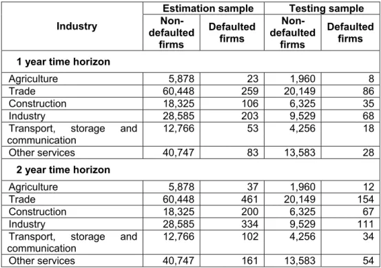
Table 1: Data structure

Estimation sample Testing sample

Industry Non-defaulted

firms

Defaulted firms

Non-defaulted

firms

Defaulted firms

1 year time horizon

Agriculture 5,878 23 1,960 8

Trade 60,448 259 20,149 86

Construction 18,325 106 6,325 35

Industry 28,585 203 9,529 68

Transport, storage and communication

12,766 53 4,256 18

Other services 40,747 83 13,583 28

2 year time horizon

Agriculture 5,878 37 1,960 12

Trade 60,448 461 20,149 154

Construction 18,325 200 6,325 67

Industry 28,585 334 9,529 111

Transport, storage and communication

12,766 102 4,256 34

Other services 40,747 161 13,583 54

According to Insolvency Law no. 85/200615, the insolvency is such state of a debtor’s private that is characterized by a shortage of available funds for the payment of debts falling. The initiation of bankruptcy procedures based on a state of “imminent insolvency” appears to be available only to the debtor itself.

3. Explanatory Variables of the Models

The data taken in account in credit scoring models shouldn’t have an exclusive accounting character, but it has to deal with all important pertinent elements. The retained variables (for company portfolios) at the beginning of the selection procedure should cover at least the classic set of the criteria used in

15 _{The Insolvency Law was published in Official} Gazette no. 359/21.04.2006.

client analysis and should particularly include: the past and future capacity to generate liquidity, equity structure, evolution of the financial results, information quality, level of indebtedness, sensitivity on the demand, ease of access to financial markets, management, competitiveness, sensitivity on country risk.

(4)

Table 2: Explanatory variables used in estimation of the models

Notation Name Definition Empirical support

ROA Return on Assets

Assets Total

Profit

Net Becchetti, L. & Sierra, J. (2003), Arshad, K. (1985)

ROE Return on Equity

Equity Profit

Net Pompe, P. &

Bilderbeek, J. (2005), Arshad, K. (1985)

Indat1 Indebtedness Rate1

Equity Debt

Total Laitinen, E. & _{Laitinen, T. (2000),} Chi, L. & Tang, T. (2006),

Indat2 Indebtedness Rate 2

Assets Total

Debt

Total Beaver, W. (1966);

Laitinen, E. & Laitinen, T. (2000) CoefCS Leverage

Equity s ' Sharholder

Assets Total

RataCpr Rate of Private Equity

Assets Total

Equity

Private Cielien, A. et al.

(2004) RotAC Current Assets Turnover

Rate Current Assets

Sales

IncasCreante Average Collection Period 360 Sales

s Receivable



RotStocuri Inventories Turnover Rate

s Inventorie

Sales Beaver, W. (1966);

Young, R. & Yue, W. T. (2005),

RotAt Assets Turnover Rate

Assets

Total

Sales

Altman, E. (1968),

Raghupathi, W. et al. (1991)

MarjaPrB Gross Profit Margin

Sales

Profit

Gross

Cielien, A. et al.

(2004); Kim, H. & Gu, Z. (2006)

MarjaPrN Net Profit Margin

Sales

Profit

Net

Beaver, W. (1966),

Kim, H. & Gu, Z. (2006)

RotCpr Equity Turnover Rate

Equity

Private

Sales

Cielien, A. et al.

(2004), Pompe, P. & Bilderbeek, J. (2005)

Disp Cash Share

Assets Current

Cash

The data collection phase is followed by the data preparing phase for the modeling. This phase might be the most complex part of the empirical estimations in case of any unpredicted problems

regarding the observations and/or the variables. The models were estimated using the STATA Data Analysis and Statistical Software.

(5)

4. Industry Level Explanations of the results

4.1. Agriculture

In case of agriculture, on one year time horizon, the rate of private equity and the indebtedness rate are the variables retained in the model, such explanatory variables for probability of

default. The statistical analysis indicates that other variables have an insignificant informational contribution for the explanation of the probability of default.

Using the two mentioned criteria for logit function estimation, the result we obtained on the estimation sample will be the one indicated below.

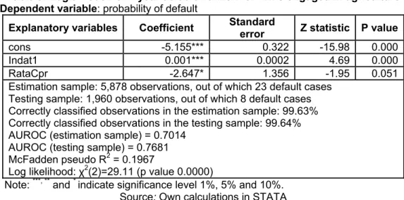
Table3:Logit model for 1 year default horizon for firms engaged in agriculture Dependent variable: probability of default

Explanatory variables Coefficient Standard

error Z statistic P value

cons -5.155*** 0.322 -15.98 0.000

Indat1 0.001*** 0.0002 4.69 0.000

RataCpr -2.647* 1.356 -1.95 0.051

Estimation sample: 5,878 observations, out of which 23 default cases Testing sample: 1,960 observations, out of which 8 default cases Correctly classified observations in the estimation sample: 99.63% Correctly classified observations in the testing sample: 99.64% AUROC (estimation sample) = 0.7014

AUROC (testing sample) = 0.7681 McFadden pseudo R2 = 0.1967

Log likelihood: χ2(2)=29.11 (p value 0.0000)

Note: ***, ** and * indicate significance level 1%, 5% and 10%. Source: Own calculations in STATA The values of the statistical tests

done on the estimation survey level reveals that the models obtained are econometrically confirmed, with statistically significant coefficients16 . The rate of private equity and the indebtedness rate have their signs according to the economical theory. The probability of default is negatively influenced by the rate of private equity, meanwhile the indebtedness rate influences in positive way17. The general explanatory power of the model is good,

16The statistical relevance of the selected criteria is also evidenced by the substantial values of the Z statistics associated with coefficients of the estimated multivariate coefficients.

17 The plus sign attached to a variable indicates an increase of the variable if the other factors remain unchanged, leading to an increase of the probability of default, meanwhile the minus sign shows the opposite influence.

taking in account the McFadden pseudo R2 with 0.196718 value.

We studied the accuracy ratio of the logit model, on the estimation and testing sample. In case we choose a cutoff point of 0.5, 99.63% of the observations are classified correctly in the estimation sample. On the testing sample the share of observations classified correctly is 99.64%.

In order to test the discriminatory power of the model we used the ROC curve and the AUROC19 indicator The results of the evaluation indicate average values of the area under ROC, both for estimation (0.7014) and testing (0.7681) samples.

The results of the estimation on 2 years time horizon are presented in

18 A value between 0.2 and 0.4 is considered a good fit.

19

(6)

Appendix 1. The determinants of defaults are: indebtedness rate, rate of private equity and cash rate. All the three variables have the expected sign and are statistically significant. In case of a cutoff point of 0.5, the share of correctly identified observations in both samples is 99.39%.

4.2. Trade

The variables which determine the probability of default on a horizon of one year in trade sector are: return on assets, indebtedness rate, rate of private equity, cash rate and the assets turnover rate. Table 4 presents the results of the estimations.

Table4:Logit model for 1 year default horizon for firms engaged in trade activities

Dependent variable: probability of default

cons -1.891*** 0.314 -6.01 0.000

ROA -0.783*** 0.265 -2.97 0.003

Indat2 -3.425*** 0.424 -8.06 0.000

RataCpr -5.507*** 0.585 -9.41 0.000

Disp -1.913*** 0.355 -5.39 0.000

RotAt -0.150*** 0.054 -2.78 0.005

Log likelihood: χ2(5) = 164.05 (p value 0.0000) Note: ***indicate significance level 1%

Source: Own calculations in STATA The coefficients are statistically

significant at a significance level of 1%. Except for the indebtedness rate all the variables have the expected sign. The probability of default is influenced in negative way all the five explanatory variables. The general degree of explanation is good taking in account the value of the indicator McFadden pseudo R2 0.2491. At the cutoff point of 0.5, 99.57% of the observations are correctly estimated in both samples. In order to test the discriminatory power of the model, the ROC curve and the AUROC indicator has been used. The results indicate average values of the area under ROC for both samples (0.7267 for the estimation samples and 0.7504 for the testing sample).

We obtained similar results with our analysis made on a 2 years horizon. All the explanatory variables and their signs remain unchanged. The share of correctly identified cases on both the estimation and testing sample are 99.24%. The results of the estimation are presented in the Appendix 2.

4.3. Constructions

(7)

firms in trade. Table 5 presents the results of the estimation on one year

horizon.

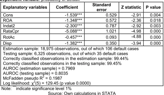
Table 5: Logit model for 1 year default horizon for firms engaged in constructions

Cons -1.539*** 0.529 -2.91 0.004

ROA -1.348*** 0.572 -2.36 0.018

Indat2 -2.300*** 0.787 -2.92 0.003

RataCpr -5.088*** 1.021 -4.98 0.000

RotAc -0.457*** 0.093 -4.88 0.000

Disp -1.382*** 0.350 -3.94 0.000

Source: Own calculations in STATA

The results of the statistical tests effectuated on the estimation sample denote that the model obtained respects the exigencies of the econometrics. The coefficients are statistically significant at 1% level. The ROA, the rate of private equity, the current assets turnover rate and the cash share have signs according to the economical theory and the indebtedness rate indicates an unexpected sign. The probability of default is negatively influenced by all five variables. The general explanation degree of the model is good, taking in account the value of the indicator McFadden pseudo R2 0.1987.

The high accuracy of the model is ensured by the scoring function in terms of discriminatory power, stability and adequate calibration of the estimations. The discriminatory power test of the sample has been done for both the estimation and testing samples. According to this, the ROC curve and the indicator AUROC have been used. The

area under ROC indicate a high value for both, estimation (0.7969) and testing (0.8035) samples. These values exceed the 0.75 reference value. In addition, the numeric results are strengthened by the form of the ROC curve.

(8)

perfect, the scores of all of the default cases would have been smaller than the non-defaulted cases.

4.4. Industry

In case of companies in industry the statistically significant explanatory

variables are the return on assets, the indebtedness rate, the rate of private equity, the cash share and the assets turnover rate on both one and two year term. (see Appendix 4.).

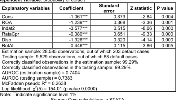
Table 6:Results of the logit model estimation on estimation sample, one year horizon (industry)

Cons -1.061*** 0.373 -2.84 0.004

ROA -1.239*** 0.368 -3.36 0.001

Indat2 -3.577*** 0.515 -8.06 0.000

RataCpr -6.080*** 0.651 -9.33 0.000

Disp -1.326*** 0.320 -4.14 0.000

RotAt -0.446*** 0.115 -3.86 0.005

The coefficients of the explanatory variables are statistically significant on 1% level of significance. Except for the indebtedness rate, all the variables have the expected sign. The probability of default is influenced negatively by all the five variables. The general explanatory degree of the model is good taking in account the value of the indicator McFadden pseudo R2 0.2638. At a cutoff point of 0.5, 99.29% of the observations are estimated correctly on both samples on one year horizon and 98.84% on 2 years horizon. Using the ROC curve and the AUROC indicator to test the discriminatory power of the model, the

area under ROC curve indicates average values for both estimation (0.7404) and testing samples (0.7383).

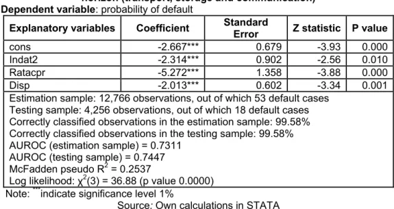
4.5. Transport, Storage and Communications

(9)

Table 7:Results of the logit model estimation on estimation sample, one year horizon (transport, storage and communication)

Error Z statistic P value

cons -2.667*** 0.679 -3.93 0.000

Indat2 -2.314*** 0.902 -2.56 0.010

Ratacpr -5.272*** 1.358 -3.88 0.000

Disp -2.013*** 0.602 -3.34 0.001

Source: Own calculations in STATA The values obtained as results of the

statistical tests effectuated on the estimation sample denote that the obtained model fulfill the requests for a good econometrical performance. The coefficients are significant at 1% level. The variables private equity rate and cash share have signs in concordance with economical theory, indebtedness rate having a different sign, all the three variables influencing the probability of failure in negative way. The general explanatory degree of the model is good, according to the indicator McFadden pseudo R2 0.2537.

In case of a 0.5 cutoff point the share of correctly identified observations is

99.58% on the estimation and testing sample. The area under the ROC curve is 0.7311 for the estimation sample and 0.7447 for the testing sample, values close to the 0.75 reference level.

4.6. Other Services

(10)

Table 8:Results of the logit model estimation on estimation sample, one year horizon (other services)

Error Z statistic P value

cons -1.919*** 0.490 -3.92 0.000

ROA -0.336*** 0.125 -2.69 0.007

Indat2 -3.999*** 0.679 -5.89 0.000

RataCpr -7.079*** 0.954 -7.42 0.000

Disp -1.920*** 0.383 -5.00 0.000

Source: Own calculation in STATA The values of the statistical tests

effectuated on the estimation sample emphasize that the model matches the exigencies of the good econometrical performance. Coefficients are significant at 1% level. ROA, private equity rate and cash share have signs in accordance with the economical literature, but indebtedness rate has an unexpected sign. The probability of default is negatively influenced by all the four explanation variables. The general explanation degree of the model is good, according to the McFadden pseudo R2 0.2782.

99.80% of the observations are identified correctly in the estimation sample and 99.79% in case of the testing sample, fact which indicates a high accuracy rate. The high accuracy of the estimations done with the model is ensured by the scoring function performance in terms of discriminatory power, stability and adequate calibration of the estimations.

The area under ROC is higher than the 0.75 reference level in case of both samples (0.7892 for the estimation sample and 0.8122 for the testing sample), the numeric exemplification

being strengthened by the form of the ROC curve as well.

Conclusions

In this paper we used logit models in order to estimate the probabilities of default for Romanian companies. The study was elaborated with the use of a sample containing 222,551 non-default non-financial companies having their financial statements in 2006 and 1,763 default companies, among which 970 defaulted in 2007, and 793 in 2008. For the estimation of our models we used data from the 2006 balance sheet and financial results of the companies. The influence of 14 indicators has been studied on one and 2 years horizon.

Variables influencing significantly the probabilities of default of the companies by industry are the following:

- Agriculture: on one year horizon private equity rate, indebtedness rate, on 2 years time horizon the two variables being completed with the cash rate.

(11)

- Constructions: ROA, indebtedness rate, private equity rate, current assets turnover and cash rate influencing the probability of default on both one and two years term.

- Transport, storage and

communications: indebtedness rate,

private equity rate and cash rate are the variables influencing the probability of default on one and two year horizon.

- Other services: on one and two years horizon the influence factors are the ROA, the indebtedness rate, the private equity rate and the cash rate.

REFERENCES

Altman, E. I. “An emerging market credit scoring system for corporate bonds”, Emerging Market Review, 2005, nr. 6, pg. 311-323;

Becchetti, L. & Sierra, J.

“Bankruptcy Risk and Productive Efficiency in Manufacturing Firms”, Journal of Banking and Finance, 2003, vol. 27(11), pg. 2099-2120;

Bhatia, M. Credit Risk Management & Basel II, An Implementation Guide, Risk Books, London, 2006;

Lizal, L. “Determinants of financial distress: what drives bankruptcy in a transition economy? The Czech Republic case.”, Wiliam Davidson Working Paper nr. 451, 2002, pg. 1-45;

Moinescu, B. Sistem de previziune a evenimentelor de deteriorare a ratingului CAAMPL, Caiete de studii, Nr. 23, BNR, 2007;

Resti, A. & Sironi, A.

Risk Management and Shareholders’ Value in Banking, John Wiley & Sons, Chichester, 2007;

***** Legea nr. 85/2006 privind procedura insolvenţei, apărută în Monitorul Oficial al României, Partea I, nr. 359 la data de 21 aprilie 2006; ***** http://www.mfinante.ro/contribuabili/link.jsp?body=/contribuabili/pjuridi

ce.htm;

(12)

Appindex 1. Logit model for 2 year default horizon for firms engaged

in agriculture

cons -4.406*** 0.268 -16.44 0.000

Indat1 0.001*** 0.0002 4.50 0.000

RataCpr -1.847*** 0.990 -1.86 0.062

Disp -2.186*** 0.998 -2.19 0.029

Estimation sample: 5,878observations, out of which 37 default cases Testing sample: 1,960 observations, out of which 12 default cases Correctly classified observations in the estimation sample: 99.39% Correctly classified observations in the testing sample: 99.39% AUROC (estimation sample) = 0.6859

Log likelihood: χ2(3)=33.25 (p value 0.0000) Note: ***indicate significance level 1%

in trade activities

cons -1.579*** 0.242 -6.51 0.000

ROA -0.729*** 0.226 -3.22 0.001

Indat2 -3.256*** 0.323 -10.06 0.000

RataCpr -5.605*** 0.446 -12.55 0.000

Disp -1.090*** 0.232 -4.69 0.000

RotAt -0.113*** 0.037 -3.01 0.003

(13)

in construction

cons -1.489*** 0.399 -3.73 0.000

ROA -1.154*** 0.431 -2.68 0.007

Indat2 -2.441*** 0.599 -4.07 0.000

RataCpr -5.138*** 0.753 -6.82 0.000

RotAc -0.191*** 0.049 -3.88 0.000

Disp -0.732*** 0.237 -3.08 0.002

in industry

cons -1.243*** 0.300 -4.14 0.000

ROA -0.807*** 0.366 -2.20 0.028

Indat2 -2.691*** 0.403 -6.67 0.000

RataCpr -4.875*** 0.502 -9.70 0.000

Disp -1.345*** 0.256 -5.25 0.000

RotAt -0.445*** 0.090 -4.90 0.000

(14)

in transport, storage and communication

Dependent variable: probability of default

cons -2.826*** 0.490 -5.76 0.000

Indat2 -1.461*** 0.627 -2.33 0.020

RataCpr -4.693*** 0.970 -4.84 0.000

Disp -0.951*** 0.363 -2.62 0.009

Appindex 6. Logit model for 2 year default horizon for firms engaged in other services

Dependent variable: probability of default

cons -1.954*** 0.364 -5.36 0.000

ROA -0.329*** 0.103 -3.20 0.001

Indat2 -2.960*** 0.479 -6.18 0.000

Ratacpr -6.758*** 0.705 -9.59 0.000

Disp -1.428*** 0.264 -5.40 0.000