Albanian j. agric. sci. 2015;14 (3): 206-213 Agricultural University of Tirana
*Corresponding author: Pëllumb R. Harizaj; E-mail: p.r.harizaj@gmail.com (Accepted for publication on September 21, 2015)
ISSN: 2218-2020, © Agricultural University of Tirana
RESEARCH ARTICLE
(Open Access)
Pricing Nature: Failing to Measure the Immeasurable
PËLLUMB R. HARIZAJ1*
1Agricultural University of Tirana, Faculty of Agriculture and Environment, Kodër-Kamëz, 1029, Tirana, Albania
Abstract
The value of Earth`s ecosystems cannot be correctly measured by monetary units as they cannot capture the infinite value nature has for humanity. A better way for valuation and protection of natural ecosystems would be the identification and quantification of nature`s buffering capacities and their corresponding tipping points for different global natural cycles, which would serve humanity as objective biophysical limits in all economy-nature interactions. These limits could be applied at different scales, from global to local in the process of decision making. This study presents also an example of the inseparable relations between the buffering capacities and their tipping points for water and carbon cycles. This example demonstrates that land biomes` buffering capacities for water cycling and carbon sequestration have reached their tipping points simultaneously in the middle of 19th century. Avoiding these negative trends requires the implementation of a massive reforestation plan at global scale within a few decades.
Keywords: nature`s buffering capacity; tipping point, value of ecosystems.
1. Introduction
The internalization of the external costs has been the logical bases of different methods for natural resources` valuation during the last several decades. These methods were designed for the good purpose of making the policy makers aware on the importance of natural resources for the prosperity of human society. Although, in principle, it has been accepted by different authors [1,2,3]that the value of natural ecosystems to the economy is infinite they have developed procedures of valuation based on the free market principles such
as, “the willingness to pay”. The valuations they have
made are expressed in finite values of many trillions of dollars (or other currencies) which, with time, keep rising to higher finite values that remain always smaller in comparison with the infinite value of the world ecosystems accepted in principle by the same authors. Although the criticism against this type of valuations has always been present [4,5,6] they didn`t succeed in changing the way the valuations of the world ecosystems are made so far. It seems that after decades of valuing world ecosystem in monetary units, a broader consensus is crystallizing: the degradation of natural resources as well as the decline of human wellbeing can be described more precisely by physical units than by monetary ones [7].
2. Material and Methods
2.1. The indifference curves for nature and human made goods
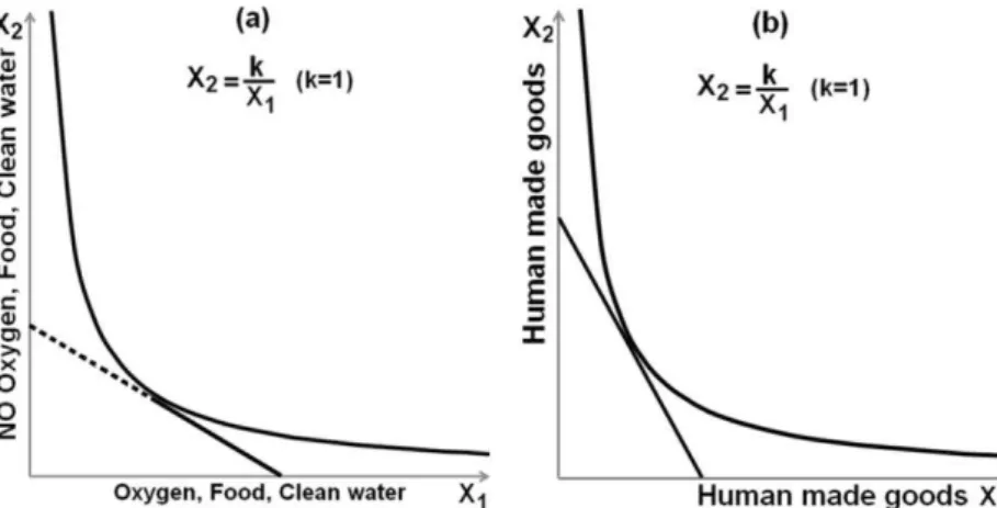
The indifference curves (refer to figure 1a, 1b) within the simplified macroeconomic cycle are based on the functionx2=k/x1 which is widely used in
microeconomics to define the indifference curves. In this formula k=1, 2, 3, 4 etc, and x1 and x2 are goods
that can be exchanged with each other[8]. The indifference curves are used in this study to define the marginal rate of substitution by the means of slopes that are tangent to them.
2.2. Calculation of the total value of the Earth`s ecosystems
For the calculation of the total value of Earth`s ecosystems the total surface of Earth is considered 510,064,472 km2 based on NASA data [9]. The
2.3. Data used in this study
The average rates of GPP, NPP production, and the land use changes in different biomes are calculated based on publications that are presented in the references list [21,22,23,24,25,26,27]. All the other data, presented in the Supplementary Information tables, are produced by the calculations made by the author of this study.
3. Results and Discussion
3.1. Substitutable and non substitutable goods
The indifference curves along with the tangent lines that define the marginal rate of substitution (MRS) of
one good by another are presented in figure 1. Figure 1a illustrates the indifference curves for three of the crucial nature`s products that are most palpable for every human being: oxygen, food and clean water. It is clear that for nature produced “goods” there are no marginal rates of substitution by other nature or human made goods, especially in the case of infinite scarcity and zero availability. In these cases the prices would be either extremely high or equal to infinity (∞).
This is not the case for any of human made goods (figure 1b). There are always possibilities to substitute one human made good with another one at different marginal rates of substitution. Human made goods are substitutable because they are not indispensible for human survival.
Figure 1. Indifference curves of utility functions and tangent lines of MRS. 1a-Oxygen, food, and clean water are non substitutable “goods”, i.e. no other goods can serve as substitutes for them. 1b-All human made goods can be substituted by other human made goods according to marginal rates of substitution (MRS) [8].
3.2. The real value of the world ecosystems
Calculation of the total value of the Earth`s ecosystems is made by multiplying the total Earth surface expressed in hectares by market prices that change according to the availability of the natural resources. By replacing in following definite integral:
∫ xdx
a=0 hectares, or zero availability of natural resources, and b=51006447200 hectares (the total Earth`s surface), the following result will always be produced:
∫ xdx = ∞
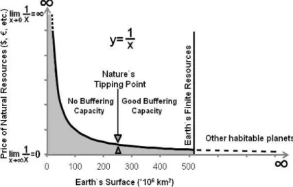
The result is infinite due to infinite prices of ecosystem services (limx→ x=∞) in the case of zero availability of non substitutable products of nature. The infinite
sign (∞) shows that the total value of the
Earth`s ecosystems expressed in monetary units ($, €,
etc.) is immeasurable. The same result would be obtained by speculating that human society would have at its disposal many other habitable planets, i.e. the natural resources would tend to be limitless (figure 2).
Comparison of values obtained by applying “the willingness to pay” with the ones obtained by
208
Figure 2. The value of Earth` ecosystems. The grey colour under the curve of function y=1/x represents the total value of Earth`s ecosystems. The interval 0–510 in the horizontal axis represents the total global surface (x106 km2). The interval 0–∞ (vertical axis) represents different market prices based on the availability of natural resources. The rate of consumption of natural resources is defined by the tipping point in which the speed of human consumption equals the nature`s speed of production. Please read the text for the explanation of concepts “buffering capacity” and “tipping point”.
1) The valuation of ecosystems services based on the market prices are mathematically incorrect. The monetary evaluations represent always finite numbers. However large they could be, these numbers remain always smaller than the infinite value the world ecosystems have for humanity. Mathematically
speaking, finite numbers can never capture the “size”
of infinity.
2) Monetary units are incommensurable with complex bio-geo-chemo-physical processes of nature which can be measured only by units employed in natural sciences.For example, oxygen and food are produced by plants through the process of photosynthesis by using as raw materials water, carbon dioxide, and sunlight. If one of these three factors of plant production would be missing the photosynthesis cannot be realized and the result would be the lack of oxygen and food at the same time. Another example is the production of clean water that is realized by the filtering ability of soil layers. If soil layers would be polluted by toxic materials, the ability of nature to produce clean water would be lost forever or might be recovered for extremely long period of times.
3) Monetary units are established since the earliest times as a means of exchange among people specialized in the production of specific goods & services. Market prices tend to represent the time and
capital spent during their production as well as the equilibrium between the supply and demand at the moment of their exchange.
This reasoning leads to the conclusion that although the monetary evaluations of Earth`s ecosystems are made for the good purpose of drawing the attention of the policy makers on the importance of nature`s ecosystem services, they represent the use of the wrong “tools” for achieving a good purpose.
3.3. Integrating Earth and Economic Systems
The concept of tipping points/thresholds in the form it is defined and applied in the existent research literature [11,12,13,14] creates serious problems [15,16]. W. H. Schlesinger summarized this problem in the following
way “Unfortunately, policymakers face difficult
decisions, and management based on thresholds, although attractive in its simplicity, allows pernicious, slow and diffuse degradation to persist nearly indefinitely. Through the Holocene, atmospheric CO2
was nearly constant; nature mitigated the effects of humans. The human impact on the carbon cycle now exceeds the natural buffering capacity of the Earth system, leading to cumulative changes in the environment for life in every corner of the planet. When these changes are more rapid than evolution, extinctions mount and the ability of the planet to
Avoiding this long term negative trend requires a redefinition of the nature`s tipping points/thresholds. For this reason this study defines the nature`s buffering capacity in natural cycles inseparably from the tipping points/thresholds.
By definition the buffering capacity of nature is its ability to lessen or moderate the impacts caused by humans or other factors.
The new definition of the tipping point/threshold in
natural processes is formulated as “the point at which a series of small changes or incidents becomes significant enough, and beyond which nature`s buffering capacity is smaller than the magnitude of
impacts inflicted by one or several causes.”
In this way the concept “tipping point/threshold”
achieves two far reaching objectives at the same time: 1) It becomes an objective warning indicator as it monitors at the same time the rate of nature`s buffering capacity to mitigate a certain negative impact inflicted by humans and the rate of this negative impact. The tipping point/threshold is reached when both rates become equal.
2) This concept, if applied in the nature-human interface (figure 3), would represent an objective biophysical limit to any human activity that can be put forward by science, and applied and monitored in effective ways by policy makers at levels that range from local to global.
Figure 3. Reservoirs and fluxes of Earth & economic systems. The indifference curves of utility functions and their tangent lines that define MRS (marginal rates of substitution) are integrated within the macroeconomic cycle. Please read text for explanations.
The integration of Earth and economic systems is realized through the tipping points. If a tipping point is reached, all the firms and households should try to find other solutions for meeting their needs for more production and consumption such as, improved management and the implementation of new innovative technologies that consume less natural resources.
3.4. Examples of buffering capacity and tipping points
Figure 4 considers the year -1700 as the time when land
biomes of Earth were “undisturbed” from human
activities. The trend of deforestation of vast areas in favour of crop land extension, since 1700, is the main cause of the reduced water buffering capacity in land biomes.
Forest biomes have two important advantages compared to other land biomes:
210 evaporation and respiration caused by plant litter decay.
Second, larger amounts of biomass production in forests (GPP, NPP) mean that larger amounts of water are released during forest respiration compared to the water released by plant respiration in other biomes. This water is part of evapotranspiration process on land and most of it becomes part of water cycle on land. The areas with higher amount of evapotranspiration have the chance to receive more rainfall, even if the annual
fresh water discharge from the oceans might be limited in these areas. These two advantages, i.e., higher water holding capacity along with higher amount of transpired water by plants, makes the forest biomes more resilient to rainfall shortages for several months during dry seasons, whereas the plants of the other biomes would suffer the most, and in the case of cultivated crops human intervention through irrigation is frequently required to avoid yield failures.
Figure 4.Past and future trends of water buffering capacity reduction. When the reduction of water buffering capacity equals the minimum fresh water discharge provided by global water cycles to land, “the tipping point” is reached. Please read text for explanations.
Around 1850 the reduction of water buffering capacity of land biomes with 20000 km3 coincided with the
minimum fresh water discharge provided annually by the global water cycle to land (The minimum fresh water discharge is ≈20000 km3/year) [17]. This
coincidence marks an important tipping point: land biomes start to become vulnerable by the lack of water. Another important fact is that this event coincides with another tipping point: the start of the unstoppable increase of atmospheric CO2 around 1850. This can be
explained by the inseparable relation between carbon and water cycles (see formulas 1 and 2 for photosynthesis and respiration in Supplementary Information). When global water discharge is at its dry season minimum (≈20000 km³/year) it limits the efficiency of photosynthesis which uses CO2, water,
and sun light to produce organic matter, and that`s why the final result would inevitably be a smaller GPP and NPP.
This lack of overlapping between the annual fresh of water discharge on land and the water needs of land biomes has been accentuated with time since 1850. In 2010 the reduction of the land biomes` buffering capacity exceeded the global average of freshwater discharge on land (38000 km3/year > 36000 km3/year),
and around 2100 the loss of buffering capacity may dangerously approach the maximum level of global fresh water discharge on land (42000 km3/year →
52000 km3/year). That means that large areas of land
biomes may no longer be able to store enough quantities of water in their soils and biomass to support normally their annual life cycles, independently from the seasonal fluctuations of global water cycles that usually range between 20000 and 52000 km3/year [17],
periods of time which would consequently result in the collapse of some of them.
This trend of global GPP and NPP decrease can remind us of similar trends in the past geological eons that are scientifically proved [18]. Comparison of the modern time (1700–2010) with a time interval in the
Permian-Triassic boundary (≈260–245 million years ago), might be especially striking: there is scientific evidence that during that ancient time the atmospheric CO2
concentration was increased due to wild fires, and the last 5 million years of that 15 million year time span, were accompanied by substantial reduction of lowland forests and swamps. This resulted in a significant reduction of the global organic matter burial and the decrease of the oxygen concentration in the atmosphere from 31% to 15% [18]. That period of time was also characterized by one of the most important massive extinctions of the last 550 million years of the Earth` history. The modern period 1700–2010 is marked by massive deforestations for obtaining more land for crop cultivation, the continuous increase of fossil fuels`
consumption, and the massive extinction of species at rates never seen before. It seems that the events of the modern time are a kind of repetition of the Permian-Triassic eon but at different speeds: the ancient events took some 15 million years to unfold whereas the modern ones are unfolding within several centuries.
4. Conclusions
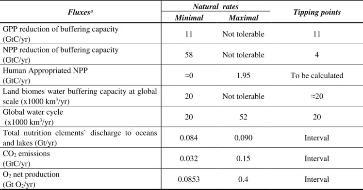
Global cycles of carbon, water, oxygen, nutritional elements, and Earth`s crust processes (subduction and uplift), are inseparably related with each other (please refer to figure 4 and supplementary table 6 for illustration). This type of mutual dependency among all cycles facilitates the identification and quantification of buffering capacities and their respective tipping points at different scales, from global to local, and offers to all people concerned (policy makers included), the right tools for taking the right decisions in relation to economic activities and environment protection (table 1).
Table 1.Buffering capacity/tipping point for some global cycles.
Fluxesᵃ Natural rates Tipping points
Minimal Maximal
GPP reduction of buffering capacity
(GtC/yr) 11 Not tolerable 11
NPP reduction of buffering capacity
(GtC/yr) 58 Not tolerable 4
Human Appropriated NPP
(GtC/yr) ≈0 1.95 To be calculated
Land biomes water buffering capacity at global
scale (x1000 km3/yr) 20 Not tolerable ≈20
Global water cycle
(x1000 km3/yr) 20 52 20
Total nutrition elements` discharge to oceans
and lakes (Gt/yr) 0.084 0.090 Interval CO2 emissions
(GtC/yr) 0.032 0.15 Interval
O2 net production
(Gt O2/yr)
0.0853 0.4 Interval
ᵃ Most of the data in the above table are based on the Supplementary Table 6 calculations and its related comments.
Applying the nature`s buffering capacity as the most objective criteria in defining the tipping points/thresholds that should be respected by all economic activities, would give humanity a chance to correct the actual seemingly inescapable trend of human made catastrophes.
212 century. It would lessen the problem of global carbon emissions and global warming, reduce the rate of species extinction, improve the water regime in all land biomes (crop lands included), which would consequently lead to yield increase without additional investments. This might be best realized if during the reforestation process the crop cultivated landscapes would be alternated by reforested areas wherever it is possible.
5. References
1. Costanza, R. The value of the world`s ecosystem services and natural capital. Nature, 387, 253-260 (1997).
2. Costanza, R. Changes in the global value of ecosystem services. Global. Envvironmenal Change, 26, 152-158 (2014).
3. De Groot, R. Global estimates of the values of ecosystems and their services in monetary units.
Ecosystem Services, 1, 50-61 (2012).
4. McCauly, D. J. Selling out on nature. Nature, 443, 27-28 (2006).
5. Vatn, A., Bromley, D.W. Choices without Prices without Apologies. Journal. of Environmental
Economics and Managagment. 26, 129-148
(1994).
6. Spash, C.L., Vatn, A. Transferring environmental value estimates: Issues and alternatives. Ecological Economics, 60, 379-388 (2006).
7. Spangenberg, J.H., Settle, J. Precisely incorrect? Monetizing the value of ecosystem services.
Ecological Complexity,7, 327-337 (2010).
8. Varian, H.R. Intermediate Microeconomics: A Modern Approach, Publisher: W.W. Norton & Company, Inc., 500 Fifth Avenue, New York, N.Y. 10110. USA (2014).
9. NASA website, Earth: Facts & Figures.
http://solarsystem.nasa.gov/planets/profile.cfm?Object =Earth&Display=Facts&System=Metric (2014). 10. Sydsaeter, K., Hammond, P.J. Mathematics for
Economic Analysis. Publisher: Prentice Hall, Inc., Upper Saddle River, New Jersey, USA (1995). 11. Scheffer, M Early-warning signals for critical
transitions. Nature, 461, 53-59 (2009).
12. Rockström, J. et al. Planetary boundaries: exploring the safe operating space for humanity.
Ecol. and Soc. 14(2), 32 (2009).
13. Barnosky, A. D. Approaching a state shift in
Earth’s Biosphere. Nature, 486, 52-58 (2012).
14. SteffenW. Planetary boundaries: Guiding
human development on a changing planet.
Science, 347, 1-10 (2015)
15. Schlesinger, W.H. Thresholds risk prolonged degradation. Nature Reports Climate Change, 3, 112-13 (2009).
16. Bass, S. Keep off the grass. Nature Reports Climate Change, 3, 113-14 (2009).
17. Syed, T.H., Famiglietti, J.S., Chambers, D.P., Willis, J.K., Hilburn, K. Satellite-based global-ocean mass balance estimates of interannual variability and emerging trends in continental freshwater discharge. PNAS, 107, 17916-17921 (2010).
18. Berner, R.A., VandenBrooks. J.M., Ward, P.D. Oxygen and evolution. Science, 316, 557-558 (2007).
19. Berner, R. A. Geocarbsulf: A combined model for Phanerozoic atmospheric O2 and CO2.
Geoch. et Cosmoch. Acta,70, 5653–5664 (2006). 20. Bonciarelli, F., Bonciarelli, U. Agronomia,
Publisher: RCS Scuola, S.p.A., Milano, Italy (2003).
21. Klein Goldewijk, K. Estimating global land use change over the past 300 hundred years: The HYDE Database. Glob. Biogeoch. Cycl., 15, 417-433 (2001).
22. Zhao, M., Heinsch, F.A., Nemani, R. R., Running, S. W. Improvement of MODIS terrestrial gross and net primary production global data set.
Remote Sens. of Environ. 95, 164-176 (2005). 23. Del Grosso, S. Global Potential net primary
production predicted from vegetation class, precipitation, and temperature. Ecology, 89 (8), 2117–2126, (2008),
24. Waugh, D. Geography: An Integrated Approach. Publisher: Nelson Thornes, Delta Place, 27 Bath Rd, Cheltenham, GL537TH, U.K. (2007).
25. Global Forest Resources Assessment 2010. Global Tables: Trends in extent of forest 1990-2010. Food and Agriculture Organization of the United Nations:
http://www.fao.org/forestry/fra/fra2010/en/
(2014).
S.K. Allen, J. Boschung, A. Nauels, Y. Xia, V. Bex and P.M. Midgley (eds.). Cambridge University Press, Cambridge, United Kingdom and New York, NY, USA, 1535 pp.
27. Earth Policy Institute http://www.earth-policy.org/?/data_center/C22/ (2012).
28. Berner, R. Burial of organic carbon and pyrite sulphur in the modern ocean: its geochemical and environmental significance. Am. Jour. of Sci. 282, 451-473 (1982).
29. Schlesinger, W.H., Bernhardt, E.S. Biogeochemistry: An Analysis of Global Change. Academic Press, Elsevier Inc., 225 Wyman St., Waltham, MA 02451, USA (2013). 30. Seiter, K., Hensen C., Zabel, M. Benthic carbon
mineralization on a global scale. Glob. Biogeoch. Cycl., 10.1029/2004GB002225 (2005).
31. Di-Giovanni, C., Disnar, J.R., Macaire, J.J. Estimation of the annual organic carbon yield related to carbonated rocks chemical
weathering: implications for the global organic carbon cycle understanding. Glob. and Planet. Change, 32, (2)195-210 (2002).
32. Falkowski, P.G.The Rise of Oxygen over the Past 205 Million Years and the Evolution of Large Placental Mammals. Science, 309, 2202-2204 (2005).
6. Additional Information
Supplementary information is available in the online version of AJAS journal at:
https://sites.google.com/a/ubt.edu.al/rssb/.
Author contributions The author is the only contributor to this work.
Supplementary Information
“Pricing Nature: failing to measure the immeasurable”
Identifying and quantifying buffering capacities and tipping points for global cycles
Due to land changes inflicted by humans in the course of history the Earth`s ecosystems have lost a part of their buffering capacity for different processes. In this study a quantification of changes that have happened in nature`s buffering capacity for Net Primary Production (NPP), Gross Primary Production (GPP), carbon cycle, and water cycle is made.
Increasing the precision in monitoring NPP, GPP, carbon, water, and oxygen cycles will enable the defining of Earth`s buffering capacity for important natural processes that are crucial for the survival of humans and other species on the planet. This would make possible to determine objectively when the tipping points are achieved and what humans must do to avoid important human induced catastrophes of nature.
Quantifying the relations among GPP, NPP, carbon, and water cycles
The cycles of NPP, GPP, carbon, and water are inseparably related with each other. The chemical formulas of plant photosynthesis and respiration illustrate this inseparable relationship:
Photosynthesis: 6(CO2) + 6(H2O) + Sunlight→ 6(CH2O) + 6O2 [1]
Mass balance: (6x44) + (6x18) → (6x30) + (6x32)
264 + 108 → 180 + 192 372 →372
72 atomic units of carbon and 108 atomic units of water participate in photosynthesis` reactions.
Respiration: 6(CH2O) + 6O2 →6 (CO2) + 6(H2O) + Heat [2]
Mass balance: (6x30) + (6x32) → (6x44) + (6x18) 180 + 192 → 264 + 108
372 → 372
72 atomic units of carbon and 108 atomic units of water are released from respiration reactions
Supplementary Table 1. Land biomes productivity (gC/m²/year)
Land Biomesᵃ Reference Year
-1700 1700 1850 1990 2010
Forest / Woodland
Surface
(x10⁶ km²) 58.6 54.4 50 41.5 40.3306 Productivity
(g C/m²/year)
GPP 1304.2 1304.2 1304.2 1342.2 1342.2 NPP 577.2 577.2 577.2 594.4 594.4
Steppe/Savannah/ Grassland
Surface
(x10⁶ km²) 34.3 32.1 28.7 17.5 17.5 Productivity
(g C/m²/year)
GPP 1160ᶜ 1160 1160 1185.5 1185.5 NPP 651.7 651.7 651.7 666 666
Shrub land
Surface
(x10⁶ km²) 9.8 8.7 6.8 2.5 3.7 Productivity
(g C/m²/year)
GPP 563 563 563 602 602 NPP 288.5 288.5 288.5 308.5 308.5
Tundra/ Hot Desert/ Ice Desert c
Surface
(x10⁶ km²) 31.4 31.1 30.4 26.9 26.9 Productivity
(g C/m²/year)
GPP 164.8 164.8 164.8 177 177 NPP 107 107 107 115 115
Crop Land
Surface
(x10⁶ km²) 0 2.7 5.4 14.7 15.1 Productivity
(g C/m²/year)
GPP 695.2 695.2 695.2 721 721 NPP 405 405 405 420 420
Pasture
Surface
(x10⁶ km²) 0 5.1 12.8 31 31 Productivity
(g C/m²/year)
GPP 373.1 373.1 373.1 396 396 NPP 244 244 244 259 259
aLand surface is adapted from Klein Goldewijk et al.2001 [21]. Calculation of average productivities (g/m2/year)
of land biomes NPP and GPP are based on Zhao et al 2005 [22].
For the years – 1700, 1700, and 1850 it is supposed that the GPP and NPP per m2 were smaller in comparison
with present time [23]. For 1990 and 2010 the increased level of atmospheric CO2 is assumed to have stimulated
the increase of plant production.
c For tundra and desert NPP is considered 140 and 90 g/m2/year respectively, and their average 115 g/m2/year. Data
Supplementary Table 2. Total amount of carbon recycled annually via land biomes (x10⁶ ton C/year)
Land Biomes Reference Year
-1700 1700 1850 1990 2010ᵃ
Forest / Woodland GPP 76,426 70,948 65,210 55,701 54,132 NPP 33,824 31,400 28,860 24,668 23,973 Steppe/Savannah/
Grassland
GPP 39,788 37,236 33,292 20,746 20,746 NPP 22,353 20,920 18,704 11,655 11,655
Shrub land GPP 5,517 4,898 3,828 1,505 2,227 NPP 2,827 2,510 1,962 771 1,141 Tundra/Hot Desert/
Ice Desert
GPP 5,175 5,125 5,010 4,761 4,761 NPP 3,360 3,328 3,253 3,094 3,094
Crop Land GPP 0 1,877 3,754 10,599 10,887 NPP 0 1,094 2,187 6,174 6,342
Pasture GPP 0 1,903 4,776 12,276 12,276 NPP 0 1,244 3,123 8,029 8,029 TOTAL GPP 126,906 121,988 115,870 105,589 105,030 NPP 62,364 60,495 58,089 54,390 54,233 NPP/GPP ratio 0.49 0.50 0.50 0.52 0.52 GPP decrease in relation
to earlier years 0.0% 3.9% 8.7% 16.8% 17.2% NPP decrease in relation
to earlier years 0.0% 3.0% 6.9% 12.8% 13.0%
aData for the total amount of forests in 2010 are based on FAO database [25]. The amount of forest decrease in
Supplementary Table 3. Carbon recycled with NPP and Human Appropriation of NPP (x10⁶ ton C/year)
Land Biomes Reference Year
-1700 1700 1850 1990 2010 2100
Forest / Woodland GPP 76,426 70,948 65,210 55,701 54,132 NPP 33,824 31,400 28,860 24,668 23,973 Steppe/Savannah/
Grassland
GPP 39,788 37,236 33,292 20,746 20,746 NPP 22,353 20,920 18,704 11,655 11,655
Shrub land GPP 5,517 4,898 3,828 1,505 2,227 NPP 2,827 2,510 1,962 771 1,141 Tundra/Hot desert/
Ice desert
GPP 5,175 5,125 5,010 4,761 4,761 NPP 3,360 3,328 3,253 3,094 3,094
Crop Land GPP 0 1,877 3,754 10,599 10,887 NPP 0 1,094 2,187 6,174 6,342
Pasture GPP 0 1,903 4,776 12,276 12,276 NPP 0 1,244 3,123 8,029 8,029
Total land biomes GPP 126,906 121,988 115,870 105,589 105,030 102,514ᵃ NPP 62,364 60,495 58,089 54,390 54,233 53,526 Human
Appropriation of NPP for food
0 547 1,935 3,087 3,171 3,549
Human
Appropriation of NPP (Industrial + fuel wood)
0 10 17 385 370 302
Total Human Appropriation of NPP
0 557 1,952 3,472 3,541 3,851
ᵃ Data for 2100 are obtained by extrapolating the differences between 2010 and 1990.
Supplementary Table 4. Water recycled in land biomes (x10³ km³ H₂O/year)
Land Biomes Reference Year
-1700 1700 1850 1990 2010 2100
Forest / Woodland GPP 115 106 98 84 81 NPP 51 47 43 37 36
Steppe/Savannah/ Grassland GPP 60 56 50 31 31 NPP 34 31 28 17 17
Shrub land GPP 8 7 6 2 3
NPP 4 4 3 1 2
Tundra/Hot Desert/Ice Desert GPP 8 8 8 7 7 NPP 5 5 5 5 5
Crop Land GPP 0 3 6 16 16
NPP 0 2 3 9 10
Pasture GPP 0 3 7 18 18
NPP 0 2 5 12 12
Total land biomes GPP 190 183 174 158 158 154 NPP 94 91 87 82 81 80 Human Appropriation of NPP for
food NPP 0.00 0.82 2.90 4.63 4.76 5.32 Human Appropriation of NPP
Supplementary Table 5. Reduction of land biomes` buffering capacity for water recycling (x10³ km³ H₂O/year, and Gt C/year)
-1700 1700 1850 1990 2010 2100 Total decrease of buffering capacity
by reduced respiration of GPP + HANPP
0 8 20 37 38 42
Decrease of buffering capacity by Human Appropriation of NPP for food and wood (HANPP)
0 1 3 5 5 6
Reduction of buffering capacity by
reduced respiration of GPP 0 7 17 32 33 37 Decrease of buffering capacity by
reduced respiration of NPP 0 3 6 12 12 13 Maximum fresh water discharge on
land 52 52 52 52 52 52
Average fresh water discharge on
land 36 36 36 36 36 36
Minimum fresh water discharge on
land 20 20 20 20 20 20
GPP (Gt C/year) 127 122 116 106 105 103
Supplementary Table 6. Carbon, water, oxygen, and chemical elements cycles (Gt/year)
Units Reference Year
-1700 1700 1850 1990 2010 2100
Total Organic Carbon
Cycled with GPP 127 122 116 106 105 103
Cycled with NPP 62 60 58 54 54 54
Organic carbon transported with water runoff ᵃ
Transported by water runoff Relative to total NPP
1.963 1.904 1.829 1.712 1.707 1.685
Organic carbon buried in river deltas
Organic carbon buried in river deltas (relative to org. carb. in water runoff)
0.150 0.145 0.139 0.130 0.130 0.128
Carbon in Human Appropriat. NPP
NPP for food and wood
& fuel 0.00 0.56 1.95 3.47 3.54 3.85
Water
Cycled with GPP 190 183 174 158 158 154
Cycled with NPP 94 91 87 82 81 80
Oxygen
Cycled with GPP 338 325 309 282 280 273
Cycled with NPP 166 161 155 145 145 143
Oxygen produced (relative to organic carbon burial in rivers deltas)ᶜ
0.399 0.387 0.371 0.348 0.347 0.342
Macro and Micro elements Cycle
Recycled within the soil (Relative to NPP carbon)
5.543 5.377 5.163 4.835 4.821 4.758
Transported by water runoff (Relative to carbon in water runoff)
0.175 0.169 0.163 0.152 0.152 0.150
Phosphorus cycle Relative to carbon in
water runoff 0.009 0.008 0.008 0.008 0.008 0.007
Nitrogen Cycle Relative to carbon in
water runoff 0.065 0.063 0.061 0.057 0.057 0.056
Potassium Cycle Relative to carbon in
water runoff 0.044 0.042 0.041 0.038 0.038 0.037
ᵃExport of organic carbon from soils to rivers for 2011 was 1.7 Giga ton Carbon/year (IPPC report 2013) [26]. This rate is converted as % relative to 2010 NPP and is applied for all the time intervals.
The influence of HANPP in the cycles of macro and micro elements used by plants is not taken in consideration as it is assumed that all these elements are returned back to rivers, oceans and lakes by the waste water discharges made by humans.
ᶜThe amount of oxygen production presented in this table is only the contribution of terrestrial plants. The amount of organic carbon produced by land NPP which is buried in deltaic areas is considered 0.13 Gt/year [28].
The organic matter that is transported by water runoff is partially oxidized on its way to oceans and lakes. The oxidation process is stopped only when the organic matter is buried deep in the sea floor. Hence the oxygen produced by the organic carbon burial (reduced carbon) is smaller than the theoretical calculations. The analyses of shelf-deltaic muds show that the annual rate of organic carbon burial is 0.13 GtC/yr [28] although at river deltas the total organic carbon transported by rivers is 0.4 GtC/year [29]. Going back to the initial carbon exported by rivers (Supplementary Table 6) the maximum efficiency of carbon burial in rivers` deltas and lakes originated from terrestrial NPP based on the year 2010 is 0.13/1.707=7.6%. Adding to the amount of organic carbon buried that is originated from land NPP, the amount of carbon buried in open oceans that is originated by the oceanic NPP (0.002– 0.12 GtC/year) [30] the total organic carbon burial would be 0.132–0.250 GtC/year. Due to the uplift and weathering of sedimentary rocks that are exposed to atmospheric oxygen, about 0.1 Gt/year of organic carbon is exposed to oxidation [31]. As a result of that the net organic carbon burial in oceans and lakes at global scale would be 0.032–0.15 GtC/year, which produces a net amount of atmospheric O2 0.0853–0.4 GtO2/year.
The increase of atmospheric oxygen for the last 205 million years, from 10% to 21% [32] reveals that during such a long period of time the net annual rate of oxygen rise in the Earth`s atmosphere has been approximately 0.00268 GtO2/year (calculated by the author of this study). Although there are still uncertainties related to the exact value
of net annual oxygen production, the range 0.0853–0.4 GtO2/year may be considered temporarily reliable, until