The Edges of Areal Units

(1)

A Case Study in the Heterogeneous Effects

of Assessment District Edges

(2)

A Case Study in the Heterogeneous Effects of Assessment District

Edges

Dissertation supervised by Prof Dr Tiago Oliveira Prof Dr Mark Padgham

Prof. Dr. Jorge Mateu

(3)

I would like to thank Dr Marco Painho for the patience, thoughtfulness, open-‐ mindedness, and support that he imbued in every facet of my academic development.

I would like to thank Professors Tiago Oliveira, Marcus Padgham, and Jorge Mateu for their patience, guidance, and support in developing this work. In particular, I would like to thank Dr Padgham for his help in making a complicated, vaguely formulated idea into a simple and testable hypothesis. I would like to thank Dr Oliveira for his instrumental role in pushing me to understand the methods and modeling necessary to test this hypothesis. I must also thank Drs Werner Kuhn and Simon Scheider for the discussions at the MUSIL seminar group at IFGI, as well as Schuyler Erle and Melissa Santos. I would also like to thank every person that I have spoken with about this work: classmates, colleagues and friends, and most of all: my family.

Finally, I am grateful to the European Commission for the Erasmus Mundus program. ISEGI, IFGI, and UJI are unique and excellent place for higher education, and I hope that the Erasmus Mundus program will continue to support all of the excellence in academic work and cross-‐cultural exchange that makes it such a rich place in which to be a student.

(4)

A Case Study in the Heterogeneous Effects of Assessment District

Edges

ABSTRACT

Areal units are used in a broad range of demographic and physical description and analysis related to surveying, reporting, navigation, and modeling. In The Modifiable Areal Unit Problem, Openshaw (1983) described how the arbitrariness of an areal unit’s boundaries means that any measurement aggregated to it is to some extent arbitrary as well. Therefore, those who survey, model, and report information based on these units must be aware of their shortcomings as models for describing phenomena that they aggregate.

Here we propose to test an aspect of the Modifiable Areal Unit Problem, namely that the boundaries used by an application of modeling with areal units are not homogeneous in their relationship to the phenomena that they model. That is, here we focus on the general problem that the boundaries of a set of areal units aren’t entirely arbitrary. Boundaries for these areal units specifically—and many others generally—are along physical and social features of the environment, which may have an internal effect on the phenomena that they describe as homogenous in the aggregate.

In this thesis, we use real estate sales data and assessor’s neighborhood boundaries to develop a method for describing differences in the effect of the boundaries of areal units. It is hoped that the methods developed here could be applied to the analysis of other urban phenomena that are restricted, afforded,

(5)

Modifiable Areal Unit Problem Spatial Ontology

Cartographic Methods Residual Analysis

(6)

Page:

1. INTRODUCTION ... 1

THEORETICAL FRAMEWORK ... 1

BACKGROUND ... 2

OBJECTIVE ... 3

HYPOTHESIS ... 4

GENERAL METHODOLOGY ... 4

DISSERTATION ORGANIZATION ... 4

2. LITERATURE REVIEW ... 5

OVERVIEW ... 5

HOUSING (HEDONIC) REGRESSION ... 5

2.3 Spatial Aspects of a Housing Model ... 6

2.4 Geographic Statistical Units ... 7

THE PSYCHOLOGY OF URBAN BOUNDARIES ... 8

3. DATA AND METHODS ... 11

STUDY AREA ... 11

POPULATION GROWTH, HOUSING, AND URBAN PLANNING (1790-‐1900) ... 11

POPULATION GROWTH, HOUSING, AND URBAN PLANNING (1900-‐2000) ... 13

HISTORY OF NEIGHBORHOODS IN WASHINGTON D.C. ... 14

HOUSING SALES (2000-‐2012) ... 17

DEMOGRAPHIC CHARACTERISTICS BY CENSUS AREAL UNITS (2010-‐2011) ... 20

HOUSE CHARACTERISTICS (2010-‐2012) ... 23

MANY VARIABLES, MULTICOLLINEARITY, AND PRINCIPAL COMPONENT ANALYSIS ... 24

PRINCIPAL COMPONENTS ANALYSIS ... 25

HEDONIC REGRESSION ... 26

VARIABLE SELECTION FOR REGRESSION MODEL ... 27

A HEURISTIC FOR EXAMINING THE SPATIAL VARIATION IN RESIDUALS AT BOUNDARIES ... 28

4. RESULTS ... 30

INTRODUCTION ... 30

REGRESSION MODEL RESULTS ... 30

RESIDUALS AND ASSESSMENT NEIGHBORHOOD BOUNDARIES ... 31

(7)

ANNEX ... 41

(8)

Figure 1 – Edges, Nodes, and Districts in Boston (Lynch, 1960) ... 10

Figure 2 -‐ English: Plan of the City of Washington, March 1792, Engraving on paper ... 12

Figure 3 -‐ Map of Present Day Washington D.C. with L'Enfants Historic Plan for "Washington City" and Washington County ... 13

Figure 4 -‐ Year of Construction of Residential Buildings in Washington DC (source: DCGIS) ... 14

Figure 5 -‐ Official and Colloquial Neighborhoods in Washington, D.C. in 1877 (Washington Post) ... 16

Figure 6 -‐ Map of Median Income by Census Tract (2011 ACS) ... 21

Figure 7 -‐ Map of % of White Population by Census Block Group (2010) ... 21

Figure 8 -‐ Map of Median Age by Census Tract (2011 ACS) ... 22

Figure 9 -‐ Map of % of Population with Bachelors Degree by Census Tract (2011 ACS) ... 22

Figure 10 -‐ Proportional and Cumulative Variance of PCA of all Variables ... 26

Figure 11 -‐ Assessment Boundaries of Interest ... 28

Figure 12 -‐ Example Boxplot of Residuals (Binned by Distance from Example Boundary) ... 32

Figure 13 – Example Selected Neighborhood, Boundary, and House Sales Locations (base data c/o OSM) ... 33

Figure 14 -‐ Map of Boundaries at which Residuals are Significantly Different ... 34

Figure 15 -‐ A Significant Boundary Adjoining a Major Road ... 35

Figure 16 -‐ Boxplot of Residuals going south from Florida Avenue ... 36

Figure 17 - Washington, DC Census Tracts ... 48

(9)

Figure 22 -‐ Boundaries with Significantly Different Adjacent Home Sale Prices (2008-‐2009) ... 50 Figure 23 -‐ Sixteen Cities Within the City (Krier, 2000) ... 51

(10)

Table 1 – Population Growth Patterns in Washington, D.C. from 1800 to 1890

(Source: US Census) ... 13

Table 2 -‐ 20th Century Population (in thousands, source: US Census) ... 14

Table 3 -‐ Demographic Characteristics Considered for Analysis ... 20

Table 4 -‐ Demographic Characteristics Summary (2010-‐2012) ... 23

Table 5 -‐ House Characteristics Data Dictionary ... 23

Table 6 -‐ House Characteristics (2010-‐2012) ... 24

Table 7 -‐ Qualitative Variable Description (2010 -‐ 2012) ... 25

Table 8 -‐ 2006-‐2007 Data Summary ... 42

Table 11 -‐ Estimated Coefficients for House Sales 2006-‐2007 ... 45

Table 12 -‐ Estimated Coefficients -‐ 2008-‐2009 Housing Sales ... 46

(11)

1. INTRODUCTION

Theoretical Framework

Areal units are used in a broad range of demographic and physical description and analysis related to surveying, reporting, navigation, and modeling. For example, the United States Census Bureau surveys and publishes information according to a nested set of areal units (e.g. Tracts, Block Groups, and Blocks). Consumer location services direct users according to areal units assigned with colloquial neighborhood names. And real estate assessors and agents model and describe the value of properties by areal units. In each of these cases, the definition of an areal unit is based on expert knowledge with a particular use model.

Census units are drawn for efficient surveying, homogeneity of demographic characteristics, and spatio-‐temporal continuity. Neighborhoods used in consumer location services are built to describe colloquial words for describing Place. And real estate assessment neighborhoods are constructed for accuracy and equity in describing how a complex set of physical and social characteristics relevant to housing are imbued with economic value.

In The Modifiable Areal Unit Problem, Openshaw (1983) described how the arbitrariness of an areal unit’s boundaries means that any measurement aggregated to it is to some extent arbitrary as well. Therefore, those who survey, model, and report information based on these units must be aware of their shortcomings as models for describing phenomena that they aggregate.

(12)

Background

Roads, parks, highways, and other physical features cut through urban areas, affording and prohibiting activity in a city. In addition, a physical feature—such as a particular street—can often serve as a named boundary or delineating feature between areas or neighborhoods.

Homogeneous Statistical Areas, such as Census Blocks often based on these boundaries. For example, the US Census explains about their areal units:

Census blocks, the smallest geographic area for which the Bureau of the Census

collects and tabulates decennial census data, are formed by streets, roads,

railroads, streams and other bodies of water, other visible physical and cultural

features, and the legal boundaries shown on Census Bureau maps. (Census, 1994)

As indicated in the text, the smallest census units are sensitive to higher-‐level areal units such as administrative boundaries. Of course, there are strong reasons to believe that these administrative units are critical determinants of the things that happen within them. Laws and taxes vary across them. And at the areal units below, we can see that significant environmental features make up their boundaries.

Other HSA’s are often based on census boundaries: real estate assessor’s neighborhoods, urban planning neighborhood clusters. In the Annex we present a comparison of these units in our area of interest.

While much has been written about HSA’s, including doing analysis based on demographic data based on them, the theory behind their construction (in urban planning or economics), the effect of scale and boundary delineation on qualitative analysis (the Modifiable Areal Unit Problem), the effect of the boundaries which define them on people psychologically, less attention has been given to how the boundaries of these HSA’s may effect the processes that occur within them.

(13)

and related urban processes. We might expect, for example, that two different kinds of boundaries have different effects.

Objective

In this thesis, we use real estate sales data and assessor’s neighborhood boundaries to develop a method for describing differences in the effect of boundaries. It is hoped that the methods developed here could be applied to the analysis of other urban phenomena that are restricted and afforded by boundaries, such as crime and movement.

(14)

Hypothesis

The aim of this work was to test the following:

1. Residential home sales can be modeled with regression

2. The residuals of said regression models reveal patterns of spatial dependence and heterogeneity in the housing market.

3. The boundaries used to model and understand spatial dependence and heterogeneity are heterogeneous in their relationship to the housing market they are used to model.

General Methodology

The general methodology of the thesis is borrowed from regression analysis for housing in economics, although it differs in overall objective. In real estate economics, there is typically a focus on the identification of the effect of a particular parameter in a global model. In the case of this thesis, we do not hypothesize that boundaries in general have an effect, but that certain boundaries may have an affect on houses that they circumscribe. Ex-‐ante, we may be able to test for the effect of these particular boundaries using regression models, but our concern here was on developing methods for first identifying those boundaries among a set that we might want to look at more closely.

Dissertation Organization

This study is comprised of five chapters. The first chapter—the introduction— includes a brief overview of the background, objective, hypothesis, and general methodology. The second chapter—the literature review—reviews relevant literature on urban planning & design, real estate economics, and homogeneous statistical areas. The third chapter provides a description of the data and the methods used to test the hypothesis, the results of which are discussed in the fourth chapter. Finally, the fifth chapter details some conclusions based on the results, discussed their academic relevance, and suggests future directions for research.

(15)

2. Literature Review

Overview

Much of this literature review will describe methods for modeling house prices. While in theory the spatial processes that describe some important facets of housing may be modeled directly, in practice many economists and assessors use homogeneous geographic statistical areas. Little is understood about how the cartographic nature of these geographic units, in particular their boundaries, relate to the processes that they circumscribe. Our hypothesis is that these boundaries are heterogeneous in their relation to the housing sales process. Because they are often drawn along common physical features of the urban environment (roads, parks, etc), we borrow some of the language of urban design to describe them.

Housing (Hedonic) Regression

First, we review applied modeling for housing economics. In the analysis section of this thesis we will use a method that is traditionall known as “hedonic” regression to hold constant all other variables as we look at the relationship between boundaries and real estate sales transactions. Sheppard (1997) provides one of the simplest definitions of the theory of how and why hedonic regression might be used.

Imagine, for a moment, that you are a private investigator or market researcher studying the demand for food. You have a particular disadvantage, however, in that you have been banned from entering the local grocer. You have found a place outside where you can sit and photograph shoppers as they approach the checkout counter, and from these photographs you can pretty much tell what foods each customer has purchased (although some items may be obscured in the shopping basket) and the total cost of all items combined. By bribing a contact at the local bank, you are able to find out each shoppers income. That is all the information that you have. From this, can you infer the demand for eggs? Can you determine how much households would be willing to pay to remove sugar import quotas? (Sheppard, 1999)

(16)

we doing food market research, we would only be interested in using the information available to us to accurately predict the price that a particular basket at the grocer would cost.

Two features of this literature motivate this approach to hedonic regression. The first feature is that the theoretical basis for the specification of the hedonic regression and the interpretation of the parameters is not well developed. As such, there is considerable variation in the variables and model specifications that are used, and little common agreement on which ones are appropriate. In turn, the success of these models is typically assessed in terms of accuracy, for house prices and for specific parameters (Malpezzi, 2003).

The second motivating feature of the review is that, in housing models, missing variables are a given, but there is a high degree of correlation among missing variables and those included in the regression. Because of this correlation, it can be difficult to interpret individual parameters. However, this high correlation among descriptive variables also means that models can be explanatory for price overall, even with missing variables. The objection that in modeling a missing variable may not be accounted for is legitimate, but in housing models, variables often proxy for one another in the overall goal of price prediction (Malpezzi, 2009). For our question in particular, the goal is in holding price, based on independent variables, consistent, so that we can inspect variation in value across space. To that extent, any set of variables that accurately holds price constant across space will be useful to us. On the other hand, location itself is a proxy for many variables, a fact we will discuss in the next section.

2.3 Spatial Aspects of a Housing Model

“Location” is a common parameter or vector of parameters in real estate modeling. However, the geographic structure of housing data is difficult to parse because it contains at least two related but distinct aspects. It can be difficult to identify the effect of one or the other in the model (Bourassa, 2003).

(17)

parameters of houses (Anselin, 2002); others map variation in parameters estimates geographically (Brunsdon, Fotheringham, & Charlton, 1996); some inspect the spatial distribution of residuals (Dubin, 1992); and most just use aggregate statistical regions and neighborhoods (Bourassa, 2003).

2.4 Geographic Statistical Units

These aggregate regions and neighborhoods might be understood to capture both the first aspect of location (dependence) and the second: that many variables that are important to housing (e.g. school, work, noise, demographics) are spatially fixed (Bourassa, 2003). For example, because one of the requirements of the establishment of new census tracts is homogeneity of demographics among the households within them, we might expect that not only is a sum of demographics described by the tract’s geography, but so too is the spatial distribution of a group of highly similar people.

Housing economists have long theorized that there are market segments in housing, and many assume that they are probably geographic (Tiebout, 1956). A market segment contains a set of goods that are substitutes, and therefore more or less similar in use value to the buyer. Assuming census tracts are homogenous, most economists have assumed that they are the best representations of market segments (Goodman & Thibodeau, 2003; Wachter & Wong, 2008).

We might thank that it better to model housing prices by areal units because demographic characteristics correspond to them. Bourassa (2003) tests this hypothesis by comparing the accuracy of two models: one, with market segments based on geographic units delineated by assessors and another, with market segments that are derived on similarity comparison across social and physical variables and then applied to houses irrespective of geographic continuity. They find that the assessor’s geographically contiguous submarket definitions are more accurate.

(18)

based on this method. She also suggests that it may be possible to create appraisal boundaries based on these surfaces. Work on the effectiveness of neighborhoods created from residuals continues, with the authors finding that “spatial trend analysis and census tract variables do not perform nearly as well as neighboring residuals(Case, Bradford, & al., 2004).

One method for accounting for the spatial error in residuals is to introduce the error into the model via a spatial weights matrix. Anselin outlines a plethora of ways to do this (Anselin, 2002). However, there is evidence that the results of the regression model become highly dependent on the characteristics of the spatial weights matrix itself. Furthermore, the methods for applying spatial weights matrices do not account for the heterogeneity in distances among houses (Bell, 2000). Given the sensitivity of our question to the heterogeneous qualities of individual neighborhoods and their boundaries, a regression model with a spatial weights matrix may obfuscate heterogeneity in service of global accuracy. In sum, there are numerous methods for account for both spatial dependence and local neighborhood qualities in a housing regression. In this thesis, we focus on the method most commonly used, that of areal units. We take the tack of many economists, modeling dependence in the form of demographic characteristics, assuming that characteristics such as age, income, race, and education as aggregated to census areal units are useful variables for describing spatial dependence as well as important qualities of a neighborhood. By using these variables, rather than a spatial regression, we elude the difficulty of having a secondary model of space, obscuring the focus on the spatial relationship between houses and boundaries.

The Psychology of Urban Boundaries

(19)

in The Image of The City. He uses a mix of personal interviews, fieldwork, and cartographic comparison to develop an ontology of urban design psychology based around: Paths, Edges, Districts, Nodes, and Landmarks. At the risk of oversimplifying: Paths allow movement, Edges inhibit it, Nodes and Landmarks may be important for ordinal sense of direction and place, and Districts are places that may be defined by all of the above, about which one can feel inside of or outside of.

His theory of Edges and Nodes was nuanced enough to capture and describe several kinds of relationships that might occur at a boundary. For example, here he is on Edges and Paths "An edge may be more than simply a dominant barrier if some visual or motion penetration is allowed through it—if it is, as it were, structured to some depth with the regions on either side. It then becomes a seam rather than a barrier, a line of exchange along which two areas are sewn together (Lynch, 1960, P 100)."

(20)

Figure 1 – Edges, Nodes, and Districts in Boston (Lynch, 1960)

(21)

3. Data and Methods

This chapter introduces the study area, the data, and the methodology for analysis. It is divided into two sections. The first introduces some general facts about Washington, D.C., its urban plan and neighborhoods, and housing. The second reviews relevant considerations about the modes of analysis and the data used.

Study Area

Washington, D.C. is the capitol city of the United States. It is an independent District with a 2010 population of roughly 6 hundred thousand. It is located within the Washington Metropolitan Statistical Area, population 5.6 million, at the southernmost tip of the US Megalopolis, population 44 million (US Census, 2010). As the center of a metropolitan region, Washington has seen waves of population gain and loss that roughly follow those of other United States cities. However, Washington has recently experienced population growth, after decades of decline.

Population Growth, Housing, and Urban Planning (1790-‐1900)

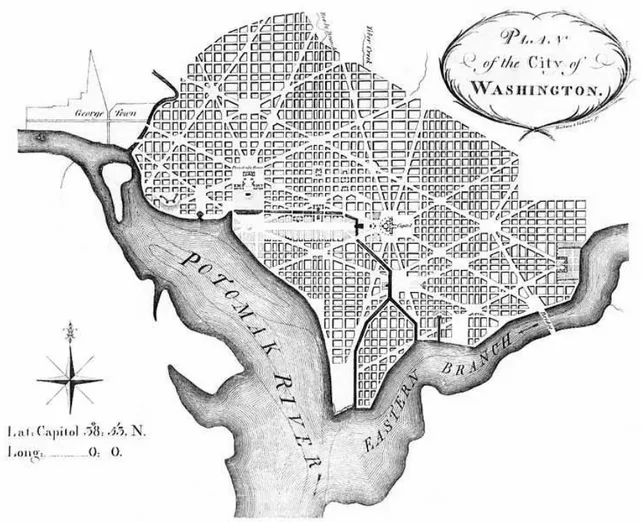
While the city saw early occupation in the form of trading posts and ports by Native Americans and then European Settlers for many hundreds of years, it only achieved the pretense of what a current inhabitant might recognize as a city within the past two hundred years. In his first major urban design project Pierre L’Enfant was commission by George Washington, the first President of the United States to design the city (Rybczynski, 2010). L’Enfant designed a plan that is still relevant to the boundaries of the city today (Figure 2).

(22)

Figure 2 -‐ English: Plan of the City of Washington, March 1792, Engraving on paper

(23)

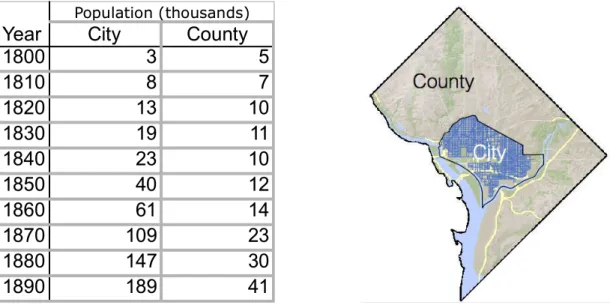
Table 1 – Population Growth Patterns in Washington, D.C. from 1800 to 1890 (Source: US Census)

Figure 3 -‐ Map of Present Day Washington D.C. with L'Enfants Historic Plan for "Washington City" and Washington County

While Historic “City” and “County” Washington kept pace through the beginning of the century, its clear that population grew much more quickly in the historic “City” starting around 1830 and continuing through 1890. Building construction data is somewhat inconsistent for these years, but population data provides us with a proxy for the history settlement in the center of Washington, D.C. mainly.

Population Growth, Housing, and Urban Planning (1900-‐2000)

As we see in Figure 3, almost all construction of new housing after 1920 takes place outside of the historic “City.” By comparing Table 2 and Figure 3, we find that a post-‐World War II population boom roughly corresponds with waves of construction across the city. These waves in construction also result in clusters of residential developments of a consistent aesthetic quality. While we will account for building age specifically in our methods, it is important to note the historical spatial clustering of development as it corresponds to population growth. Building age has been shown in the literature review to be an important dimension along which housing markets may be segmented.

(24)

Figure 4 -‐ Year of Construction of Residential Buildings in Washington DC (source: DCGIS)

Table 2 -‐ 20th Century Population (in thousands, source: US Census)

History of Neighborhoods in Washington D.C.

(25)

of the word neighborhood is not our focus, it is hoped that this introduction will provide the reader with more historical understanding of what a neighborhood is historically in Washington. This history is relevant to our purposes because assessment neighborhoods share some historical spatial similarity and continuity with colloquial and official neighborhood names. However, it is perhaps more important for our purposes to note that colloquial and official neighborhoods can also change dramatically in name and spatial extent over time.

Given that the majority of Washington’s population in 1887 was within the L’Enfant Plan area, the neighborhood names available to us from that time, for that area, provide us with a useful starting point to understanding the dynamics of DC’s neighborhoods historically. The persistence of colloquial neighborhoods might be thought of as the persistence of a name and of the spatial extent that it refers to (Maue, 2013).

(26)

Figure 5 -‐ Official and Colloquial Neighborhoods in Washington, D.C. in 1877 (Washington Post)

On the other hand, most of the other colloquial neighborhood names from this map are not presently used, with the exception of Swampoodle, which is used in the Gazetteer of Yahoo! Inc., but it is very rarely—if at all—used in present day colloquial language. The installation of a major trans-‐city train station in the middle of historical Swampoodle in 1907 (Amtrak History and Archives, 2013) may account for why what was once considered an identifiable geographic area lost its usefulness. We will see later that this train line forms an important present-‐day boundary for real estate in the city.

(27)

neighborhoods. In these cases, the Nodes were actually a kind of improvement on the pre-‐existing historical plan that coincided with residential investment.

The historical plan for historical Washington is still important in the city’s definition of neighborhoods today. When describing Washington’s communities present-‐day Planners have described it as “Sixteen Cities Within the City. (Figure 20-‐Appendix)” Here was can see again that the boundaries for these communities are largely drawn along the historic boulevards of the city plan. Later, when we look at assessment neighborhoods and census tracts, these boulevards will predominate as lines along which borders are drawn.

Neighborhoods in Washington, D.C. are defined in large part according to an urban planning history, although they critically depend upon residential investment. In addition, their names are also defined according to the uses of those who refer to them. In Washington, colloquial names and planned neighborhood improvements often—though not always—change together, shifting into new neighborhoods according to the Edges and Nodes that prohibit and enable activity within the city. Our goal in this thesis is to determine whether residential housing purchases relate to the Edges defined by assessment neighborhoods in present day. As such, in the next section we turn to more recent developments in residential real estate investment.

Housing Sales (2000-‐2012)

In this section, we will broadly review the temporal and spatial dimensions of the housing sales transactions process that we considered in our analysis. Housing sales data, collected for tax purposes, represent a complex, multidimensional process.

(28)

Figure 7 -‐ Sales Prices of Houses from 2010-‐2012 with city Quadrants

(29)

Figure 8 -‐ Median Sales Price (2000-‐2012, Source: DCGIS, OTR)

(30)

Demographic Characteristics by Census Areal Units (2010-‐2011)

In our analysis, we assume that demographics are one of the key descriptors of

how markets are spatially and socially segmented. Demographic characteristics

were selected from the 2010 US Census and the American Community Survey

2011 3-‐year estimates. The latter were available at the census tract, and the

former at census block group (see chart). We chose all available variables that

were identified in the literature review as variables known to explain variation

in house prices.

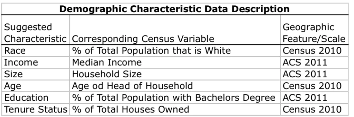
Table 3 -‐ Demographic Characteristics Considered for Analysis

Below, we map these demographic characteristics. Our goal in presenting maps

of them is twofold: 1) to give the reader a better understanding of the

geographies at which these important variables are available and 2) As discussed

in the literature review, housing economists have found that demographic

characteristics may be a direct or indirect (via signaling) explanation for local

spatial autocorrelation. Therefore, we also present demographic data by census

(31)

Figure 6 -‐ Map of Median Income by Census Tract (2011 ACS)

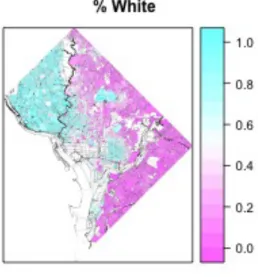
Figure 7 -‐ Map of % of White Population by Census Block Group (2010)

Both median income and percent white population might seem to explain a

significant amount of the spatial distribution in house prices. However, their

(32)

Figure 8 -‐ Map of Median Age by Census Tract (2011 ACS)

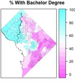
Figure 9 -‐ Map of % of Population with Bachelors Degree by Census Tract (2011 ACS)

While it is unsurprising that Median Age of the head of the household does not

seem to correspond spatially to sales prices, we include it in the later principal

component analysis and then regression analysis because, as discussed in the

literature review, there is evidence that housing markets are segmented by age.

On the other hand, the percent of the population with Bachelor’s degrees seems

to be collinear with Median Income and Percent of Population that is White. We

will speak in more depth about dealing with such colinearity in the methods

(33)

Since our dependent variable is the sale price of an individual house, we

interpolate all demographic characteristics to the house. Therefore, summary

statistics in Table 4 describe demographic characteristics of houses that were

sold. Note that variables are defined in Table 3.

Table 4 -‐ Demographic Characteristics Summary (2010-‐2012)

House Characteristics (2010-‐2012)

We use variables on characteristics of houses to describe heterogeneity in home

prices as it relates to amenities of the house itself. Records of home sales and the

characteristics of the houses sold are available from the DC Office of Tax and

Revenue. For our initial model, the selected houses sold between January 1, 2010

and Feb 28th, 2012. It later became obvious that we could also use 2 other

samples of house sales from 2006 to 2007 and from 2008 to 2009 in order to

further test both the model and our results. Summary data for these years is

presented in the Annex.

Table 5 -‐ House Characteristics Data Dictionary

Grade and Condition are both qualitatively assigned by assessors as part of the

assessment process, which includes field inspections based on outlier detection

(34)

its maintenance. Condition refers to the maintenance condition. Estimated year

built is based on a weighting system of the most recent year of major renovation

and the first year that the house was built (Office of Tax and Revenue, 2013).

Table 6 -‐ House Characteristics (2010-‐2012)

It is evident from the summary statistics that the median house was first built in

1927, underwent major renovations by 1961 or after, has 3 bathrooms, 7 rooms,

3 bedrooms, 1 kitchen, no fireplace, and has more square footage of built area

than the land on which it sits. There are, of course, extreme houses with as many

as 13 fireplaces, 12 bathrooms, and at least one house that was just a shell.

Many Variables, Multicollinearity, and Principal Component Analysis

Given the large number of variables, we had to consider ways of reducing the

number of dimensions that describe housing. Furthermore, because many of

these variables are collinear, and because our eventual mode of analysis is

dependent upon linear regression, we attempted to use Principal Component

Analysis(PCA). In the regression stage, the meaning of these principal

components became unclear, in cases in which all regression independent

variables were principal components, and in mixed models. However, we did

find that some of the transformations of the data for the regression into their

ordinal equivalents were still useful. As such, we describe them below.

One challenge in using Principal Component Analysis was identifying which of

the many characteristics of a house could be considered ordinal. In particular,

the architectural qualities of the building (e.g. a row middle, row-‐end, or

(35)

exterior wall type (e.g. stone, stucco, vinyl) do not have an immediate ordinal

identification. However, we do have access to previous sales records, which

indicate the relative value of these qualities. Since we are interested in

explaining variation in price, we can use the observed previous value of these

characteristics to construct an ordinal relationship among them. The table below

shows summary statistics for the relative value of these variable types. One can

interpret each number as a dollar value per square foot for the qualities that the

house has. For example, the median house is a row-‐house (middle), which

according to analysis of previous sales is assessed at $117 per square foot (Office

of Tax and Revenue, 2013).

Table 7 -‐ Qualitative Variable Description (2010 -‐ 2012)

Principal Components Analysis

While the loading of the variables on the principal components did not leave us

confident in our ability to interpret the results of a regression based on them,

Principal Component Analysis did reveal some useful collinearities that we later

use to better understand confusing signs on several regression coefficients.

The first three Principal Components explain 14% of the variance. Gross Building

Area (House Size), Land Area, and Median Income are the only variables that

load on these components (See PCA Table). Median income is the only variable

loaded on the first component. It explains 4.5 percent of the cumulative variance.

It is interesting to note that the orthogonal second and third components

describe the complex relationship between land area(LA) and Gross Building

Area(GBA), where GBA and LA can vary together, but also inversely.

In the DC Assessor’s manual (2012), it is pointed out that Land Area has a

complex relationship to Price, which they describe by the neighborhood that a

(36)

value of each addition square foot of land is modeled by one of four possible

elasticity curves. This model is borne out by the PCA.

Figure 10 -‐ Proportional and Cumulative Variance of PCA of all Variables

Hedonic Regression

Our method for holding all housing characteristic constant as we examine the

effect at boundaries is regression. As discussed in the literature review,

regression applied in the sense that we use it is called “hedonic” in the

economics literature.

In linear form, the hedonic regression is a regression of price onto

characteristics. That is, for , a vector of housing characteristics, the

regression is:

Equation 1 -‐ Hedonic Regression

, where are coefficients and are independent and identically distributed.

In general, the literature suggests that using a log-‐linear form of regression is

preferred for simple regression (Malpezzi, 2003). The reason that this form is

preferred is that, theoretically, it allows coefficients to vary together. That is, by

exponentiation of the observed housing variables, their effect is mutually

informative for price, rather than simply being a linear relationship between

(37)

Variable Selection for Regression Model

We evaluated several methods for modeling house prices using physical and

social characteristics. A model based entirely around PCA and around mixed PC’s

and variables left us with less confidence in our model than the linear model

based on variables. However, all three methods generally identified similar

boundaries. Because the regression model based on variables is more

informative to the reader, we present the results of that model in the results

section and include the PCA-‐based regression models in the Appendix.

Principal Components Analysis was theoretically desirable given the large

number of collinear variables. However, many of the variables load alone on a

single component, and the interpretation of the others was unclear. In light of

literature that suggests that PC’s cannot be selected for regression by the size of

their eigenvectors alone, and that all PC’s must be considered in terms of their

explanatory power for the desired variable (Jolliffe, 1982), we found that PC’s

did not provide us with a model about which we could be any more confident in

explaining than the traditional linear model based on variables themselves.

This left us with the problem of variable selection. We used stepwise regression

over 3 different pairs of years to identify a set of variables to use in the

regression model. Stepwise regression uses a series of F-‐Tests to determine

whether variables can be said to have an effect on the accuracy of the model that

is significantly different from zero (Mickey, 1967). We attempt to overcome the

shortcoming of stepwise regression, that models constructed by it may be less

generalizable (Whittingham, 2006), by applying it over 3 sets of years and

reviewing the results in the context of variables recommended in the literature

review.

For each of the three pairs of years of houses sold, stepwise regression identified

the same 19 variables. Only Crime was not identified as significant via an F-‐Test

for the 2008-‐2009 and 2010-‐2011 home sales data. However, because crime was

identified for the 2006-‐2007 data, we include it in the regression model applied

(38)

A Heuristic for Examining the Spatial Variation in Residuals at

Boundaries

As discussed in the literature review, the analysis of the spatial distribution of

residuals has been shown to be a valid method for developing better modeling

techniques for housing prices.

We developed a simple technique for inspecting the variation in residuals and

their distance from the boundary. After modeling with regression, we inspect

residuals for each house in each neighborhood with respect to their distance

from every boundary for that neighborhood.

The first step in this analysis was identifying boundaries of interest. We chose to

use only boundaries internal to the District of Columbia. This decision was

driven by the initial hypothesis that house price residuals at boundaries might

exhibit discontinuities. In the final analysis, this choice also removes the possibly

confounding factor of boundaries of a different administrative order. However, it

is also possible that future research could focus in particular at how state

boundaries relate to house prices. Prices are certainly discontinuous across state

boundaries, given differences in tax rates and services. However, since our focus

was on the internal effect of boundaries, we focused on those boundaries within

DC.

(39)

We define a boundary as a continuous line between adjacent assessment

neighborhoods. Above we plot the 235 boundaries within the District of

Columbia that make up assessment neighborhoods. 40 of these boundaries were

less than 100 meters and therefore removed from the analysis. That left 195

boundaries. Because each boundary has two sides, a total of 390 boundaries

were analyzed with respect to the residuals for houses sold within their

assessment neighborhoods.

(40)

4. Results

Introduction

In this chapter we present the results of the regression model, the relationship of

residuals at neighborhood boundaries to those boundaries, and finally, maps and

boxplots for residuals for houses for which we can be confident that there is a

difference in residual value with respect to the boundary.

Regression Model Results

The results of the regression model are shown in the Linear Model Regression

Results tables in the Appendix for all 3 pairs of years of home sales.

Of the variables that describe the physical house, all variables display the same

sign and similar magnitudes for the sign, despite summary statistics that at times

show very different underlying distributions for the data. For example, the

distribution of Land Area in 2010-‐2011 is very positively skewed and with high

kurtosis. However, the estimated coefficient is very similar in magnitude to 2006

and 2007 sales.

Estimated coefficients for social variables are more difficult to interpret. For

example, in all 3 sets of years, median income (mdninc) is estimated to have a

negative coefficient. One possible explanation for this result is that an expansion

in demand resulted in some submarkets with lower median income overall to

experience increases in price, and a larger volume of sales. In addition, the sign

on median age flips from 2006-‐2007 to 2008-‐2009. In this case, the

interpretation is not as worrisome. In the literature review, we found that

median age might be seen simply as a way that people shop in the market, and

while its bearing on price may not be direct, it is useful to us because it describes

a dimension along which people purchase homes. Percent White (pwhite) is

useful to the model in the same way. In all sets of years, educational attainment

(pbchlr—Percentage of population with a Bachelors Degree) exhibits a positive

sign. In this latter case, the direct relationship between the coefficient and the

(41)

Dummy variables on Condition and Grade are generally easy to interpret and are

consistent with expectations. For Use Code dummy variables (E.G.

USECODE012), the base comparison is against row-‐houses. The interpretation

here may be a bit confusing, because we might assume that a row house will

always be less desirable than a detached or semi-‐detached house. The estimated

coefficients generally do not indicate that this is the case. However, many of the

row houses in Washington, D.C. are historic, and may be desirable for their

historic character. Therefore, the implicit positive sign on row houses may be

understood in light of the explicit negative sign on Actual Year Built (ayb) which

we find in the regression for all years. Indeed, in the PCA, we see complex

interaction between these variables represented by the loadings on components

6 and 7. Thankfully, we are not interested in the most accurate estimate for the

coefficient on these variables, but only on their overall accuracy in predicting

price. As explained in the literature review, any missing or latent correlation at

play here should not hinder our overall goal of accuracy in price.

Residuals and Assessment Neighborhood Boundaries

Our method for relating residuals to boundaries was to use distance from a given

boundary as a dimension along which residuals might vary.

By way of example, in the figure below, we plot a histogram for residuals for all

houses within an individual assessor’s neighborhood, binned by distance from a

given boundary. Further examples can be found in the Annex.

(42)

Figure 12 -‐ Example Boxplot of Residuals (Y Axis) Binned by Distance from Example Boundary (X

Axis)

In this case, we can see that the residuals for houses in the first 2 distance bins

have actual sales prices that are consistently higher than their predicted price,.

In the following, we plot the sale point of each house, the assessor’s

neighborhood that it falls in, and highlight the boundary of interest for this

(43)

Figure 13 – Example Selected Neighborhood, Boundary, and House Sales Locations (base data c/o

OSM)

This boundary adjoins a natural park, like many of the other boundaries at which

nearby houses displayed a significantly different mean residual than the others

houses within the same assessment neighborhood.

While boxplots provide a method for inspecting boundaries and residuals

individually, we needed a method that would allow us to describe variation in

the residuals with respect to boundaries for the city as a whole. After a review of

hundreds of boxplot residuals, we settled on defining “nearby” houses as those

within the first 15% of the furthest distance from the boundary. Then we

compared the mean residual value of houses “nearby” to a boundary with the

mean residual for the rest of the houses within the assessment neighborhood.

Below we plot the boundaries at which this t-‐test resulted in a p value of less

The Edges of Areal Units

A Case Study in the Heterogeneous Effects

of Assessment District Edges

A Case Study in the Heterogeneous Effects of Assessment District

Edges

A Case Study in the Heterogeneous Effects of Assessment District

Edges

ABSTRACT

1. INTRODUCTION

Theoretical Framework

Background

Objective

Hypothesis

General Methodology

Dissertation Organization

2. Literature Review

Overview

Housing (Hedonic) Regression

The Psychology of Urban Boundaries

3. Data and Methods

Study Area

Population Growth, Housing, and Urban Planning (1790-­‐1900)

Population Growth, Housing, and Urban Planning (1900-­‐2000)

History of Neighborhoods in Washington D.C.

Housing Sales (2000-­‐2012)

Demographic Characteristics by Census Areal Units (2010-­‐2011)

House Characteristics (2010-­‐2012)

Many Variables, Multicollinearity, and Principal Component Analysis

Principal Components Analysis

Hedonic Regression

Variable Selection for Regression Model

A Heuristic for Examining the Spatial Variation in Residuals at

Boundaries

4. Results

Introduction

Regression Model Results

Residuals and Assessment Neighborhood Boundaries

Population Growth, Housing, and Urban Planning (1790-‐1900)

Population Growth, Housing, and Urban Planning (1900-‐2000)

Housing Sales (2000-‐2012)

Demographic Characteristics by Census Areal Units (2010-‐2011)

House Characteristics (2010-‐2012)