c
Uma Publicação da Sociedade Brasileira de Matemática Aplicada e Computacional.
Subspace Identification for Industrial Processes
S.D.M. BORJAS1, DCEN, Universidade Federal Rural do Semi-árido, UFERSA,
Campus Mossoró, Av. Francisco Mota 570, Bairro Costa e Silva, 59625-900 Mossoró, RN, Brasil.
C. GARCIA2, Escola Politécnica da Universidade de São Paulo - EPUSP,
Av. Prof. Luciano Gualberto, trav. 3, nr. 158 - Butantã, São Paulo, SP, Brasil.
Abstract. Subspace identification has been a topic of research along the last years. Methods as MOESP and N4SID are well known and they use the LQ decomposi-tion of certain matrices of input and output data. Based on these methods, it is introduced the MON4SID method, which uses the techniques MOESP and N4SID.
Palavras-chave. Subspace identification, state space models.
1.
Introduction
Nowadays, an engineer’s work consists more and more of obtaining mathemati-cal models of the studied processes [15]. A major part of the literature referring to system identification deals with how to find polynomial models as Prediction Error Methods (PEM) and Instrumental Variable Methods (IVM). In case of com-plex systems, the state space model appears as an alternative to PEM and IVM models [22]. For multivariable systems, these methods provide reliable state space models directly from input and output data. As systems of large dimensions are usually found in industry, the application of subspace identification algorithms in this field is very promising [3, 8, 10, 14, 16, 17, 24]. Each subspace identification method is different from the other ones in concept, interpretation and computa-tional implementation. An identification generalization is presented in [18]. In [9] a comparative study among the three most commonly used algorithms, i.e., Canonical Variate Analysis (CVA) [13], Multivariable output-Error State sPace (MOESP) [21] and Numerical algorithms for Subspace State Space System IDentification (N4SID) [19] was made. For further details about these algorithms, the reader can consult [2, 6, 7, 12, 17, 21, 22, 23, 4].
In this work it is shown, in a summarized form, the operation of POMOESP [20] and N4SID [19] methods. Combining these methods, it is obtained the MON4SID algorithm, which estimates the extended observability matrix in the same way that POMOESP method; the state sequence is computed through the oblique projection as is done in N4SID method; from this sequence it is obtained the past and future
states and finally a consistent estimate of the system matrices is obtained applying the least squares method.
Other form for integrating these methods can be found in [11], in which the au-thor aimed at reducing the computational complexity, dividing MOESP and N4SID algorithms in modules, separating them in independent parts. Afterwards, he used the computationally fastest modules of each algorithm.
1.1.
Subspace identification
Linear time invariant systems models, operating in discrete time, are dealt with in the dynamic subspace identification methods. These systems can be described by models in the innovation form
x(k+ 1) = Ax(k) +Bu(k) +Ke(k) (1.1)
y(k) = Cx(t) +Du(k) +e(k), (1.2)
where the symbols represent the inputu(k)∈ ℜm, the outputy(k)∈ ℜl, the state
x(k)∈ ℜn and the Kalman filter gain K. e(k)∈ ℜl, is zero-mean Gaussian white noise and independent of past input and output data. A,B,C, andDare matrices with appropriate dimensions.
1.2.
Subspace identification problem
The subspace identification problem: given u(k) and y(k) a set of input-output measurements aims to, determine the ordern of the unknown system, the system matrices (A, B, C, D) up to within a similarity transformation and Kalman filter gainK [19].
1.3.
Subspace matrix equation
Performing successive iterations in equation (1.1) and (1.2), one can derive the following matrix equation
Yf = ΓiXf +HidUf+HisEf, (1.3)
where subscriptf stands for the “future” andpfor the “past”. The matricesHd i and
Hs
i are defined as
Hid=
D 0 · · · 0
CB D · · · 0 ..
. ... . .. ...
CAi−2B CAi−3B · · · D
, (1.4)
His=
I 0 · · · 0
CK I · · · 0 ..
. ... . .. ...
CAi−2K CAi−3K
· · · K
The past and future input block-Hankel matrices are defined as
Up=
u0 u1 · · · uj−1 u1 u2 · · · uj
..
. ... . .. ...
ui−1 ui · · · ui+j−2
, (1.6)
whereUp, andUf ∈ ℜmixN. The output and noise innovation block-Hankel matrices
Yp, eYf ∈ ℜlixN and Ep, and Ef ∈ ℜmixN, respectively, are defined in a similar way to (1.4). The states are defined as
Xp = X0= x0, · · · xj−1 , (1.7)
Xf = Xi= xi, · · · xi+j−1
. (1.8)
The extended observability matrixΓi is given by
Γi=
C CA
.. .
CAi−1
. (1.9)
1.4.
Orthogonal projection
The orthogonal projection of the row space ofAxinto the row space of Bx is, [19],
Ax/Bx = AxBx(BxBxt)†Bx, (1.10)
where(.)†denotes the Moore-Penrose pseudo-inverse of the matrix(.). The projec-tion of the row space ofAxinto the orthogonal complement of the row space ofBx is, [19],
Ax/B⊥x = Ax−Ax/Bx. (1.11)
1.5.
Oblique projection
The oblique projection of the row space ofG along the row spaceH into the row space ofJ is, [19],
G/HJ = [G/H⊥].[J/H⊥]†.J . (1.12)
Properties of the orthogonal and oblique projections
Ax/A⊥x = 0, (1.13)
Ax/AxCx = 0. (1.14)
2.
Identification Methods
2.1.
MOESP identification Method
Inside the MOESP family, there is the POMOESP method, which solves the problem in section 1.3, by means of an approximation of the extended observability matrix Γi. Therefore, it is necessary to eliminate the last two terms in the right hand side of equation (1.3). That is done in two steps:
First, eliminating the termHd
iUf in (1.3), performing an orthogonal projection of equation (1.3) into the row space ofU⊥
f yields
Yf/Uf⊥ = ΓiXf/Uf⊥+HidUf/Uf⊥+HisEf/Uf⊥. (2.1)
By the property (1.11) it results inUf/Uf⊥= 0. Equation (2.1) can be simplified to
Yf/Uf⊥ = ΓiXf/Uf⊥+HisEf/Uf⊥. (2.2)
Second, to eliminate the noises in (2.2), it is defined an instrumental variableZ = [Ut
pYpt]t. Multiplication of (2.2) byZ yields
Yf/Uf⊥Z = ΓiXf/Uf⊥Z+HisEf/Uf⊥Z . (2.3)
As it is assumed that the noise is uncorrelated with input and output past data [20], that means thatEf/Uf⊥Z= 0.Therefore, (2.3) is written as
Yf/Uf⊥Z = ΓiXˆf. (2.4)
In equation (2.4)Xf/Uf⊥Z = ˆXf is the estimate of the Kalman filter state. Equa-tion (2.4) indicates that the column space of Γi can be calculated by the SVD decomposition ofYf/Uf⊥Z. For further details, see [19].
2.2.
N4SID identification method
N4SID method solves the problem in section 1.3 by means of an approximation of past and future Kalman filter state sequence. From the Theorem 12 in [19],
˜
Xi = Γ†iΘi, (2.5)
where Θi = Yf/UfWp which is achieved by performing an oblique projection of
equation (1.3), along the row spaceUf onto the row space ofWp, that is
Yf/UfWp = ΓiXf/UfWp+H
d
iUf/UfWp+H
s
iEf/UfWp. (2.6)
It is easy to see that the last two terms of equation (2.6) are null, Uf/UfWp = 0
by the property of the oblique projection, equation (1.12); Ef/UfWp = 0 by the
assumption that the noise is uncorrelated with input and output past data [19]. Thus, equation (2.6) can be simplified to
whereX˜i=Xf/UfWp andWp= [U
t
pYpt]t. Then equation (2.7) is written as
Θ = ΓiX˜i. (2.8)
Equation (2.8) indicates that the column space ofΓi can be calculated by the SVD decomposition ofΘandΓi can be calculated as, [19],
Γi=U1S
1/2
1 . (2.9)
Once are knownΘand Γi, it is easy to compute X˜i (calculated from (1.6)). Now ˜
Xi+1 can be calculated as, [19],
˜
Xi= Γ†i−1Θi+1, (2.10)
whereΘi+1=Yf−/U−
f W
+
p andΓi−1 denotes the matrixΓi without the lastl rows. For further details, see [19] or [6].
2.3.
MON4SID identification method
In this subsection, it is presented the MON4SID method. To solve the problem in section 1.3, it is used the POMOESP method to calculate the extended observability matrixΓi and the N4SID method is employed to calculate the matrices (A, B,C,
D) through the least squares method.
Γi, given in (2.4), can be derived from a simple LQ factorization of a matrix constructed from the block-Hankel matricesUf,Upand Yf ,Yp, in the form
Uf Wp Yf =
L11 0 0
L21 L22 0
L31 L32 L33
Q1 Q2 Q3
, (2.11)
and the orthogonal projection in the left side of (2.4) can be computed by matrix
L32 [20]. The SVD ofL32can be given as
L32=
U1 U2
=
Sn 0
0 S2 Vt 1 Vt 2
=U SVt. (2.12)
The ordernof the system is equal to the number of non-zero singular values in
S. The column space ofU1approximates that ofΓi in a consistent way [20], that is
Γi=U1. (2.13)
The system (1.1)-(1.2) can be written as
˜
Xi+1 Yi|i
= A B C D ˜ Xi
Ui|i
+ r1 r2 . (2.14)
Therefore, the problem now is to find the state sequences. The oblique projection Θi given in equation (2.8) can be computed from (2.11) by
Θi=Yf/UfW p=L32[L32]
−1
L21 L22
Q1 Q2
. (2.15)
An estimate of the state sequenceX is given by
Γi= Γ†iL32[L32]−
1
Wp. (2.16)
The following matrices are defined: X˜i =X(:,1 :N−1), X˜i+1 =X(:,2 :N).
Thus, the system matrices can be estimated from equation (2.14). The Kalman gain K can be estimated from [19] or [20]
K= [G−AP CT][Λ0−CP CT]−1, (2.17)
where P is the forward state covariance matrix, which can be determined as solution of the forward Riccati equation
P =AP AT + [G−AP CT][Λ0−CP CT]−1[G−AP CT]T. (2.18)
We have then the following algorithm
Algorithm MON4SID
1) Compute the matricesUf, Up and Yf, Yp and the LQfactorization given in (2.11).
2) Compute the SVD of the matrixL32from (2.11).
3) Determine the system order by inspection of the singular values inSgiven in (2.12).
4) Determine Γi from equation (2.13) and the state sequence X from (2.16), determine Xi+1 and Xi. 5) Compute the matrices A, B, C, and D from equation
(2.14).
3.
Simulation
In this section it is employed the Shell benchmark [5], [25] to evaluate the perfor-mance of the MON4SID algorithm and to compare it with other existing identifica-tion algorithms (PEM, MOESP and N4SID). The Shell benchmark is a model of a two-input two-output distillation column. The inputs are overhead vapor flow (D) and reboiler duty (Q); the outputs are column pressure (P) and product impurity (X). The model of the process is given as follows
P(t) = −0.6096 + 0.4022q −1
1−1.5298q−1+ 0.5740q−2D(t) +
−0.1055 +−0.0918q−1
1−1.5298q−1+ 0.5740q−2Q(t) +
+ N s
ep(t) is the white noise which generates the disturbance in the pressure. The pa-rameter N s is used to set the noise level in the simulation. For this study three values are used: 0.2, 0.5 and 1 and they are called 20 % , 50 % and 100 % noise level simulation. The standard deviation of the noise is 1.231. The model of the impurity (X) is slightly nonlinear. It is given by
X(t) = 0.0765 500000
Q(t−7)−1500+ 0.9235X(t−1) +
+ N s
1−1.6595q−1+ 0.6595q−2ex(t), (3.2)
where ex(t) is white noise with standard deviation 0.677. The Shell benchmark works around the nominal values Dnom = 20 ; Qnom = 2500; Pnom = 2800;
Xnom = 500. It was used a PRBS signal which is persistently exciting of any finite order, obtaining sufficiently informative open-loop experiments. It was col-lected 1000 samples, 800 samples were used for estimation and the remaining 200 samples were used for validation. The pre-treated signals were of the form
Fx= (F−Fnom)/(std(F))where F can beD, Q, P orX.
4.
Model Order Estimation
There is an extensive literature on algorithms to estimate the model order of a linear system in state space. In the subspace algorithms the determination of the model order nis very subtle. Ideally, this information can be determined by the number of singular values different from zero of the orthogonal or the oblique projections of row spaces of the Hankel’s block matrix of input and output data. Nevertheless, when the system data contains noise, this number is not easy to calculate. In Figure 1, it is shown the spectrum of SVD values of the process with different values of Ns. Another procedure is to select the value n, which minimizes the estimation errors, a technique used by algorithms such as PEM, which requires a higher computational effort. There is a statistical criterion that can help obtaining the model order: the Akaike Information Criterion (AIC), defined in [1],
AIC(n) =ρ.ln[σ2
error(n)] + 4Pn, (4.1)
whereρis the number of samples used in the identification,σ2
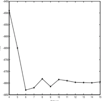
error(n)is the variance of modeling error for a model of ordernwith Pn parameters. The index AIC(n) normally reaches a minimum for a certain number of parameters in the model. The application of theAICcriterion to the process with Ns = 0.2 is shown in Figure 2, where one can observe that the minimum value occurs forn= 6.
5.
Model Performance
0 5 10 15 10−3
10−2 10−1 100 101
Order (n)
SVD
N1=0.2 N3=0.5 N2=1
Figure 1: Spectrum of SVD for different values of Ns.
4 5 6 7 8 9 10 11 12 13 14 15
−6850 −6800 −6750 −6700 −6650 −6600 −6550 −6500 −6450
Order (n)
AIC
Figure 2: Spectrum of AIC with Ns = 0.2.
a criterion to measure the distance between the model and the real system. Per-formance indicators very used are mean relative square error (MRSE) and mean related variance (MVAF), which are defined as
M RSE(%) = 1
l
l
X
i=1
v u u t
N
X
j=1
(y−yˆ)2/
N
X
j=1
(ˆy)2. 100, (5.1)
M V AF(%) = 1
l
l
X
i=1
1−var(y−yˆ)/var(y). 100, (5.2)
n= 6), Table 2 (forN s= 0.5and ordern= 6) and Table 3 (forN s= 1and order
n= 7).
Table 1: Numerical results of algorithm performance forN s= 0.2.
Algorithm Processing time(s) MRSE (%) MVAF (%)
N4SID 0.703 2.7623 99.7376
MOESP 0.312 7.0001 98.4672
MON4SID 0.407 2.4367 99.7670
PEM 3.609 7.5114 98.9544
PEM (n=7) 4.953 2.3579 99.7364
Analyzing the values of Table 1, the MON4SID model is the best one in terms of cross validation. It is verified that the processing time to obtain the model is smaller for MOESP and is much larger for PEM. The MON4SID model was chosen to identify the Shell benchmark process, due to the good balance between its performance and processing time. The PEM model gives better performance withn= 7.
Table 2: Numerical results of algorithm performance forN s= 0.5.
Algorithm Processing time(s) MRSE (%) MVAF (%)
N4SID 0.672 3.5803 99.3617
MOESP 0.297 5.3490 98.3046
MON4SID 0.400 2.9910 99.4758
PEM 0.3594 3.5728 99.3316
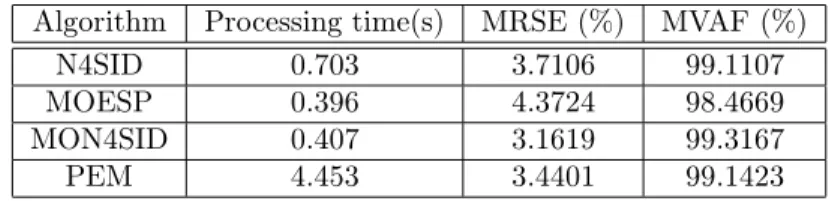
Table 3: Numerical results of algorithm performance for N s= 1 .
Algorithm Processing time(s) MRSE (%) MVAF (%)
N4SID 0.703 3.7106 99.1107
MOESP 0.396 4.3724 98.4669
MON4SID 0.407 3.1619 99.3167
PEM 4.453 3.4401 99.1423
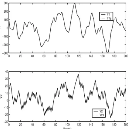
Figure 3 shows the outputs generated by the process and by the identified model for N s= 0.2. It can be observed that, for a given operating range, the identified model reproduces very well the main dynamic characteristics of the Shell benchmark process. Zero initial conditions were considered.
0 20 40 60 80 100 120 140 160 180 200 −300
−200 −100 0 100 200 300
Y1
Y1 Y1s
0 20 40 60 80 100 120 140 160 180 200 −30
−20 −10 0 10 20 30 40
Y2
time(s)
Y2 Y2s
Figure 3: Comparison of process response (broken line) versus MON4SID model response (continuous line).
6.
Conclusions
In this work, it was presented the MON4SID algorithm, which uses LQ factorization in the same way as the MOESP method, which is used to compute the oblique and orthogonal projections; given these projections it is computed the state sequence and the extended observability matrix, respectively. The past and future state sequences are computed from the state sequences which have only one initial state, it does not happen in the N4SID method, since for each oblique projection (Θiand Θi+1) different state sequences (X˜i+1andX˜i) are computed, generating a problem of bias in the estimates. To evaluate this algorithm, three identification algorithms (MOESP, N4SID, PEM) were applied to the Shell benchmark process, to identify a MIMO model in discrete time state space and their results were compared. It is possible to observe that a linear model can provide a good description of a non-linear system within a certain operating range. The Akaike criterion provided the model order. The performance comparison was made according to cross validation for each algorithm, employing two different performance criteria. For this specific case, the MON4SID model was chosen, due to its performance and processing time. PEM was the slowest model out of the four tested ones. The obtained model is observable, controllable and asymptotically stable within a certain range of operation, and it can be applied in control and monitoring applications.
Resumo. Identificação por subespaços tem sido um tema de pesquisa ao longo dos últimos anos. Métodos como MOESP e N4SID são bem conhecidos eles usam a decomposição LQ de certas matrizes de dados de entrada e saída. Com base nestes métodos, é apresentado o método MON4SID, que usa a técnica dos métodos MOESP e N4SID.
References
[1] H. Akaike, Information theory and an extension of the maximum likelihood principle. In: Second International Symposium on Information Theory, Bu-dapest, Hungary. (B.N. Petrov, F. Csaki, eds.), pp. 267–281, 1973.
[2] T. Backx, “Identification of an Industrial Process: A Markov Parameter Ap-proach”, Ph.D. Thesis, Technical Univ. Eindhoven, The Netherlands, 1987.
[3] S.D.M. Borjas, C. Garcia, Subspace identification using the integration of MOESP and N4SID methods applied to the Shell benchmark of a distilla-tion column, artigo aceito 9th Brazilian Conference on Dynamics Control and their Applications DINCON 2010, Serra Negra/SP Brasil, pp. 57, 2010.
[4] S.D.M. Borjas, C. Garcia, Modelagem de FCC usando métodos de identificação por predição de erro e por subespaços,IEEE América Latina, Revista virtual - na Internet,2, No. 2 (2004), 108–113.
[5] B. Cott, Introduction to the Process Identification, Workshop at the 1992 Canadian Chemical Engineering Conference, Journal of Process Control, 5, No. 2 (1995), 67–69.
[6] K. De Cock, B. De Moor, Subspace identification methods, in Contribution to section 5.5, Control systems robotics and automation of EOLSS, UNESCO En-cyclopedia of life support systems, (Unbehauen H.D.), 1 of 3, Eolss Publishers Co., Ltd., Oxford, UK, pp. 933–979, 2003.
[7] B. De Moor, P. Van Overschee, W. Favoreel, Algorithms for subspace state space system identification - an overview, In Applied and computational con-trol, signal and circuits, (B. Datta Ed.), Vol. 1, pp. 247-311. Birkhauser: Boston (Chapter 6), 1999.
[8] W. Favoreel, B. De Moor, P. Van Overschee, Subspace state space system identification for industrial processes,Journal of Process Control,10, No. 2-3 (2000), 149–155.
[9] W. Favoreel, S. Van Huffel, B. De Moor, V. Sima, M. Verhaegen, Comparative study between three subspace identification algorithms,Niconet, 1998.
[10] B. Haverkamp, Efficient implementation of subspace method identification al-gorithms,Niconet, 1999.
[11] B. Haverkamp, M. Verhaegen, “SMI Toolbox: state space model identifica-tion software for multivariable dynamical systems”, Vol. 1, Delft University of Technology, The Netherlands, 1997.
[13] W. Larimore, Canonical variate analysis in identification, filtering and adaptive control, In “Proc. 29th Conference on Decision and Control”, Hawai, USA, pp. 596–604, 1990.
[14] W. Larimore, Automated multivariable system identification and industrial applications, In: “American Control Conference, ACC’99”, San Diego, CA, Proceedings, Vol. 2, pp. 1148–1162, 1999.
[15] L. Ljung, “System Identification Theory for the User”, Prentice Hall Englewood Cliffs, NJ, 1999.
[16] G. Mercere, L. Bako S. Lecouche, Propagator-based methods for recursive sub-space model identification, Signal Processing,88, No. 3 (2008), 468-491.
[17] P. Roberto, G. Kurka, H. Cambraia, Application of a multivariable input-output subspace identification technique in structural analysis, Journal of Sound and Vibration,312, No. 3 (2008), 461–47.
[18] P. Van Overschee B. De Moor, A unifying theorem for three subspace system identification algorithms, Automatica, (Special Issue on Trends in System Identification),31, No. 12, (1995), 1853–1864.
[19] P. Van Overschee B. De Moor, “Subspace Identification for Linear Systems: Theory, Implementation, Applications”, Dordrecht: Kluwer Academic Publish-ers, 1996.
[20] M. Verhaegen, P. Dewilde, Subspace model identification. part i: the output-error state-space model identification class of algorithms,International Journal of Control,56, No. 1 (1992) 1187–1210.
[21] M. Verhaegen, Identification of the deterministic part of MIMO state space models given in innovation form from input-output data,Automatica(Special issue on Statistical Signal Processing and Control) ,30, No. 1, (1994) 61–74.
[22] M. Viberg, Subspace methods in systems identification. In: 10th IFAC Sympo-sium on System Identification, SYSID’94, Copenhagen, Denmark, Proceedings, Vol. 1, pp. 1–12,1994.
[23] M. Viberg, Subspace-based methods for the identification of linear time-invariant system.Automatica, (Special Issue on Trends in System Identifica-tion),31, No. 12 (1995), 1835-1851.
[24] M. Viberg, Subspace-based state-space system identification,Circuits, Systems and Signal Processing, 21, No. 1 (2002), 23–37.