Computer Simulations of Statistical Models
and Dynamic Complex Systems
J.S. S´a Martins and P.M.C. de Oliveira
Instituto de F´ısica, Universidade Federal Fluminense, Av. Litorˆanea s/n, Boa Viagem, Niter´oi, Brazil, 24210-340
Received on 10 May, 2004
These notes concern the material covered by the authors during 4 classes on the Escola Brasileira de Mecˆanica Estat´ıstica, University of S˜ao Paulo at S˜ao Carlos, February 2004. They are divided in almost independent sections, each one with a small introduction to the subject and emphasis on the computational strategy adopted.
1
Introduction
This article is an expanded version of the notes used by the authors in the course taught in the 2004 edition of the Brazil-ian School of Statistical Mechanics (EBME), held in Febru-ary of 2004 at the S˜ao Carlos campus of the State University of S˜ao Paulo (USP). The various sections are mostly inde-pendent of each other, and can be read in any order. Dif-ferent styles and notations, independently adopted by each author while writing their first versions, were kept.
The subject of all sections can be interpreted as the same, in a broad sense, namely the consequences of lacking multi-ple characteristic scales (time, size, etc) in both equilibrium statistical models (two next sections), and complex dynamic systems (remainder sections).
2
Percolation
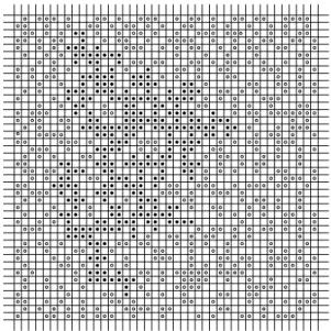
Mathematicians prefer to define percolation starting from an infinite lattice. For simplicity, let’s consider a square lattice. Each site is randomly tossed to be present or absent, accord-ing to a fixed concentrationp. By considering links between nearest neighbour present sites, one studies the structure of clusters (or islands) which appears. Fig. 1 shows a piece of such a lattice, as an example.
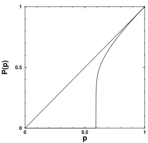
This system presents a phase transition, when one varies the concentrationp. For small enough values ofp, all islands are finite, including the largest one (highlighted by black cir-cles in Fig. 1). Starting from any present site, it is impossible to go too far away from this point by walking only through nearest neighbouring present sites: eventually one returns back to the starting point. On the other hand, by increas-ingp, suddenly the largest cluster becomes infinite, at a very precise critical valuepc, and then one can cover infinite dis-tances starting the walk from any present site belonging to this cluster. The parameter of order for this transition can be defined as follows. One takes a site at random, and measures the probabilityP(p)that this site belongs to the largest clus-ter. Forp < pc, this largest cluster being finite on an infinite lattice, this probability vanishes. Forp > pc, however, this
probability monotonically increases. Fig. 2 shows the qual-itative behaviour of this parameter. Near pc (above), this order parameter is given by
P(p)∼(p−pc)β for 0< p−pc<<<1 ,
whereβis a universal critical exponent, which depends only on the lattice dimension, not on the local lattice geometry (its valueβ = 5/36, for instance, is the same for square, triangular or any other two-dimensional lattice). The thresh-oldpc = 0.59274621(13)[1] is valid for the square lattice. However, this is not a universal quantity: the triangular lat-tice, for instance, haspc = 1/2. See [2] for this and other interesting issues.
0 0.5 1
p
0 0.5 1
P(p)
Figure 2. Probability for a random site to belong to the largest cluster.
Many further different quantities can be considered. One of then is the correlation functionG(x), defined as follows. For a given configuration like that on Fig. 1, one takes two sites distantxfrom each other, and counts g = 1 if they belong to the same clusterexcluded the largest one, other-wise one countsg = 0. Then, one takes many other pairs of sites distant the same valuex, and perform the average of
g. Finally, one considers many other configurations tossed under the same concentrationp, and perform the configura-tion average. For fixedpand large values ofx, this function exponentially decays as a function ofx,
G(x)∼e−x/ξ(p) for large x and p6=pc ,
where the so-called correlation length ξ(p) measures the range of correlations, or, alternatively, the typical diameter of an island. Even the lattice being infinite, one does not need to consider distances larger thanξ(p): a finite piece of the lattice, larger than this size, presents the same behaviour as the whole infinite lattice.
0 0.5 1
p
0 50 100
ξ
0.4 0.6 0.8 100
102
104
Figure 3. Correlation length (typical diameter of an island).
The exponential form above is only the asymptotic lead-ing factor ofG(x). Exactly atp=pc, however, long-range correlations appear, i.e. ξ(p)diverges, Fig. 3, and another leading factor emerges, namely the power-law
G(x)∼x−η for large x and p=p
c .
For lattice dimensions other thand = 2, the critical expo-nent isd−2 +η, instead. Again, the critical exponent η
is universal (in two dimensions, η = 5/24). Contrary to the exponential decay which defines the typical length ξ, this power-law lacks any characteristic length scale. Atpc, any finite piece of the infinite lattice is not enough to de-scribe its complete critical behaviour: correlations overflow the boundaries of this piece, whatever is its finite size. For this and any other critical system, the classical perturbation approach of determining first the behaviour of a small piece of the system, including later the influences of all the rest (the “perturbation”), does not work at all: the “rest” is never negligible.
Near butnotexactlyatthe thresholdpc, the correlation length itself incorporates this criticality as
ξ(p)∼ |p−pc|−ν for |p−pc|<<<1 ,
whereν is another universal critical exponent (in two di-mensions,ν = 4/3). Note the importance of excluding the largest cluster from the above definition of correlation func-tion: the correlation length remains finite below as well as above the thresholdpc. By further increasing pabovepc, some finite islands glue on the already existent infinite clus-ter, and the average diameter of the remainder islands de-creases. Fig. 3 shows the qualitative aspect ofξ(p). The exponentνis the same on both sides ofpc. The multiplica-tive factors of |p−pc|−ν omitted from the last equation, however, are two different constants.
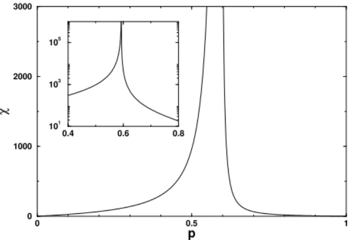
Another interesting quantity is the mean cluster size
χ(p), the average number of sites belonging to each island, again excluding the largest cluster. Assigning a unit “mass” to each present site, this quantity can be interpreted as the typical mass of an island. It reads
χ(p)∼ |p−pc|−γ for |p−pc|<<<1 ,
whereγis the corresponding critical exponent, also univer-sal (in two dimensions,γ= 43/18). The qualitative plot for
0 0.5 1
p
0 1000 2000 3000
χ
0.4 0.6 0.8 101
103
105
Figure 4. Mean cluster size (typical mass of an island).
All these quantities are related to the average number
ns(p)ofs-clusters per site, wheresdenotes the cluster size, or mass. The order parameter, the correlation length, the mean cluster size and others can be obtained from ns(p), which is then called thepotential orgeneratingfunction. (The term “per site” means to consider an enormous lattice piece, and divide the counting by the number of sites inside it, i.e. ns(p)is indeed the density ofs-clusters.) In particu-lar, atpcthis size distribution follows a power-law,
ns(pc)∼s−τ ,
whereτ is another universal exponent (in two dimensions,
τ = 187/91). Again, the system lacks any characteristic
size scale: atpc, one cannot neglect clusters larger than any predefined cut off.
Near but not exactly atpcand for large sizess,ns(p)is a generalised homogeneous function [3] ofp−pcand1/s, i.e. it obeys the property
n[Λσ(p−p
c),Λs−1] = Λτ n(p−pc, s−1) ,
whereΛis an arbitrary number, andσis a further critical, also universal exponent (in two dimensions, σ = 36/91). The critical point corresponds to both variablesp−pc and
1/svanishing. By choosingΛ =s, one obtains
ns(p) =s−τ f[(p−pc)sσ] ,
which allows an interesting interpretation. By measuring
ns(p)in units ofns(pc), i.e. by takingns(p)/ns(pc), one does not need to consider it as a function of two vari-ables pand s: it depends only on the single combination
z= (p−pc)sσ.
The order parameterP(p), Fig. 2, for instance, is related tons(p)through
p=P(p) +X
s
s ns(p) .
The reasoning behind this formula is simple. For a fixed sizes, one can determine the probabilitys ns(p)of picking a random site belonging to somes-island. (Why? First, one
counts the total number ofs-islands and multiply with s, getting the total number of sites belonging to alls-islands. Then, one divides the result by the total number of lattice sites, getting the quoted probability. Remember thatns(p) is the number of s-islands per site.) Thus, the sum over
swhich appears in the above equation corresponds to the probability of picking a random site belonging to any fi-nite island (of course, only finite values ofs are scanned by this sum.) Finally, the concentrationpof present sites is the probability for a random site to belong either to the infinite cluster (if any) or to any other island, obtained by summing up the probabilitiesP(p)andP
ss ns(p)of each case, respectively. In Fig. 2, the region above the curve for
P(p)and below the straight45o-diagonal corresponds just
to all sites belonging tofiniteislands.
The mean cluster size χ(p) is also related to ns(p) through
χ(p) =X
s
s2ns(p) ,
which rid off further explanations.
BothP(p)andχ(p)are one-site averages, obtained by scanning the lattice site by site. Thus, for each site, the prob-abilitys ns(p)to belong to somes-island is considered in the two last equations. The correlation length ξ(p) is dif-ferent, it is a two-site average. In this case, one needs to scan all pairs of lattice sites which belong to the same is-land. The class ofs-islands contribute, then, with a weight proportional to s2n
s(p). (Why? The probabilitys ns(p) to pick the first site inside this class is multiplied with the number s−1of remainder sites of the same island: any of them could be the second site, in order to form a pair. For large islands,sands−1can be confounded.) Instead of determiningξ(p) directly from the correlation function
G(x) ∼ e−x/ξ(p), one can compute a related quantity
de-noted here with the same symbolξ(p)by
ξ2(p) =
P
sRs2 s2ns(p) P
ss2ns(p)
,
whereRs measures the average radius: for eachs-island, one first computes its gyration radius defined by R2 = P
iri2/s, where ri is the distance between site i and the center of mass, and then averages over alls-islands.
At a first glance, one is tempted to relate the average mass to the average radius through the Euclidean relation
mass ∼ radiusd. However, percolation clusters are not compact objects. Instead, they arefractalswith dimension
Da little bit smaller then the Euclidean dimensiond. Thus, the correct relation ismass ∼ radiusD. Nearpc, a typ-ical fractal island with radiusξ has massξD smaller than the volumeξd, due to the holes which characterise the frac-tal. The volume fractionξD/ξdactually occupied by this is-land equals the probabilityP(p). From this equality, namely
P =ξD/ξd, one finds the scaling relation
D=d−β/ν .
the s-sums into integrals, a procedure valid near the criti-cal point, and by profitting from the generalised homoge-neous form ofns(p)in order to change the variable froms
toz = (p−pc)sσ, one can find various other scaling rela-tions between critical exponents, for instance
α= 2−τ−σ1 ,
β =τ−2
σ ,
γ= 3−τ
σ ,
δ= 1 + γ
β ,
D= d
τ−1 ,
Dσ= 1
ν ,
ν d= τ−1
σ ,
γ= (2−η)ν ,
etc. Exponentsαandδ concern respectively the tempera-ture dependence of the specific heath, and the magnetic field dependence of the magnetisation. They were not directly treated in the present text. The corresponding equations were included above for completeness. Indeed, these var-ious critical exponents are not independent from each other: knowing two of them, for instance τ andσ, one automat-ically knows all others. Equivalently, the many power-law dependences which characterise the critical behaviour are related to each other.
Contrary to mathematicians, physicists prefer finite lat-tices, for instance aL×Lsquare, a lattice piece like that shown in Fig. 1. It is treated by choosing some artificial rule to define the neighbourhood along its boundary. A particu-larly convenient rule is to take the bottom-row spins to re-place the missing up-neighbours of the top-row. Symmetri-cally, one chooses the top-row spins as down-neighbours of the bottom-row. This rule is usually called periodic bound-ary condition, the lattice becoming a cylinder. One ad-vantage is the preserved translation symmetry, all rows are rigorously equivalent. Considering also periodic boundary condition along the vertical direction, all columns equiva-lent, the cylinder turns into a torus.
The infinite lattice limit is considered by including the lattice size as a further parameter1/Linto the generalised homogeneous relation, the so-called finite-size-scaling hy-pothesis
n[λ1/ν(p−pc), λDs−1, λL−1] =λd+D n(p−pc, s−1, L−1) ,
whereλis an arbitrary number related to the previous one byΛ =λD. From this, one can express the densityns,L(p) ofs-clusters as
ns,L(p) =s−τf[(p−pc)sσ, s/LD] ,
a function of only two variables z = (p− pc)sσ and
w = s/LD, instead of p,s andL. In particular, exactly atpc, one can perform integrals inwinstead ofs, getting a series of useful finite-size-scaling relations
χL(pc)∼Lφχ =Lγ/ν ,
PL(pc)∼LφP =L−β/ν ,
ξL(pc)∼Lφξ =L ,
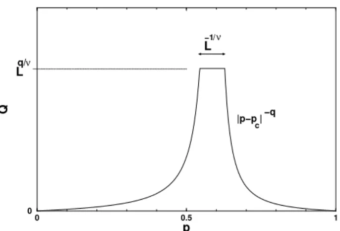
etc. The exponentφχ = γ/ν is called theanomalous di-mensionof the corresponding quantityχ(p),φP =−β/νis the same for the order parameterP(p), etc. Not surprisingly, the correlation length shares the same dimensionφξ = 1of the length finite sizeL, last relation. It has an interesting in-terpretation, normally used as an argument in favour of the finite-size-scaling hypothesis: instead of diverging atpc, the plot ofξ(p)for a finite lattice presents a peak nearpc, the height of which is proportional to the lattice lengthL.
Figure 5 gives the qualitative behaviour of some generic quantityQ(p)which diverges atpc, for an infinite lattice, ac-cording to its characteristic critical exponentq, i.e.Q(p)∼ |p−pc|−q. The plot, however, corresponds to a finite lattice of lengthL. The divergence is replaced by a cut off peak, withQL(p) ≈ Lq/ν for values of pinside an interval of widthL−1/ν aroundpc. If the thresholdp
c is known, one can profit from this finite-size behaviour in order to deter-mine the anomalous dimension φQ = q/ν, by measuring
QL(pc)for different lattice sizes. An estimate forpcitself can be also obtained, by tuning the precise concentration for which the log-log plot ofQagainstLis a straight line.
0 0.5 1
p
0
Q
Lq/ν
|p−p |−q
c
L/
−1ν
The finite-size-scaling form
Q[λ1/ν(p−pc), λL−1] =λ−φQ Q(p−p
c, L−1)
exhibits the anomalous dimension φQ for this quantityQ. By choosingλ=L, one reveals an interesting property: the plots ofQL(p)/QL(pc)against(p−pc)L1/ν will collapse on the same curve for different lattice sizesL. This equation is obtained by performing the propers−integration on the finite-size-scaling relation.
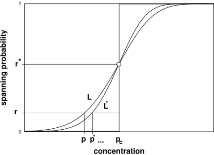
Particularly useful are quantities with vanishing anoma-lous dimension,φQ = 0. Plotted againstL, they are asymp-totically constant for large values of L, when the correct concentration p = pc is chosen. The so-called Binder cu-mulant [4] and the correlation between opposite surfaces [5] are general examples of these quantities. For percolation, one has the spanning probabilitySL(p)around, say, the hor-izontal direction. For a fixed L×Lfinite lattice, it varies with the concentration pas a sigmoid curve schematically shown in Fig. 6.
0.3
concentration
0 1
spanning probability
r
p r*
pc p,... L
L,
Figure 6. Spanning probability for two lattice sizes L andL′ (L′ > L). Due to its anomalous dimensionφ
S = 0, for larger and larger lattices this function approaches the stepS(p < pc) =
0; S(pc) =r∗; S(p > pc) = 1, also highlighted by two heavy straight lines plus the open dot. By fixing an arbitrary valuerat the vertical axis, one finds the sequencep,p′. . . for increasing lattice sizes, which converges topc.
In the limit of infinite lattice size, this curve approaches a step function, suddenly jumping from 0 (valid for allp < pc) to an isolated universal valuer∗
exactly atp=pc. Then, it immediately jumps again fromr∗
to 1 (which remains for all
p > pc). It is a kind of order parameter, vanishing along all the disordered phase. However, instead of gradually increas-ing accordincreas-ing to the smooth curve(p−pc)βwhen the thresh-old is surpassed, it becomes immediately constant along all the ordered phase, i.e. it behaves as(p−pc)0, with a zero ex-ponent instead ofβ. Thus the anomalous dimension ofS(p)
is φS = 0, whereasφP = −β/ν for the order parameter
P(p).
A simple an efficient way to get the value ofpcis to ex-trapolateSL(p)for larger and larger lattices. By fixing some
valueron the vertical axis of Fig. 6, one measures the cor-responding values pL1, pL2, pL3 . . . for increasing lattice
sizesL1,L2,L3. . . In [6], the formula
pL(r) =pc+ 1
L1/ν h
A0(r) +A1(r)
L +
A2(r)
L2 +. . . i
,
is proposed for theL-dependence of this series. The fitting of this form to real Monte Carlo data is excellent, giving numerical estimates for the thresholdpcwithin an accuracy of one part in 106, for an acceptable computational effort
[6]. One can fix any value ofrat the vertical axis, Fig. 6. The rate of convergence is dictated by1/L1/ν, for increas-ing values ofL.
A faster rate of convergence, and hence a better accu-racy, can be obtained by choosingr=r∗
, the critical univer-sal value which in some cases is exactly known through con-formal invariance arguments. Within this convenient choice, one has A0(r∗) = 0 in the above equation, accelerating
the convergence rate to1/L1+1/ν [6]. Better yet is to con-sider the probability of wrapping along the torus, instead of spanning. In this case, the convergence rate is dictated by1/L2+1/ν, and the already quoted best known estimate
pc= 0.59274621(13)was reported [1].
In [6], the spanning between two parallel lines distant
L/2from each other is verified: one countss= 1if there is some island linking these two lines,s= 0otherwise. Then,
SL(p)is the configuration average ofs. This definition mul-tiplies the statistics by a factor ofL: for the same configura-tion, one considers rows 1 and1 +L/2, also 2 and2 +L/2, etc, and repeats the same for columns. Larger lattices can be monitored in this way, allowing for instance a much better definition of the threshold distribution tails [7].
The canonical way to simulate the percolation problem on computers corresponds to a fixed concentrationp. Ac-cording to this value, one tosses a random distribution, then measures the quantityQof interest for this particular con-figuration, and finally tosses many other configurations and repeats the whole process. At the end, one has a single av-erage valueQ(p)for the fixed concentrationp. In order to get the whole functionQ(p), one needs to repeat the pro-cess for many other values ofp. Even so, the result is not a continuous function ofp.
Here, we will show a way to get the continuous depen-dence betweenQandp[1]. One starts with an empty lat-tice. Then, the lattice is filled-up, one random site at each step. After each new site, one determines the valueQn of the quantity of interest, where n is the number of present sites so far, and accumulates it on an-histogram. When the lattice is completely filled with all itsN sites present, one starts the same process again, from the empty lattice. After a sufficient large number M of repetitions, one divides all
N+ 1entries of the histogram byM: now it stores the “mi-crocanonical” averagesQn, i.e. the averages ofQfor fixed numbersn= 0, 1, 2. . . N of present sites.
Q(p) = N X
n=1
CNn pn(1−p)N −n Q
n ,
F
D G L
K
F D G L
K
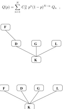
Figure 7. Tree structure of cluster labels. The root for this par-ticular cluster is siteK. In order to find the ultimate label for site F, one needs a two-step search, because it does not point directly to the root (up). Once this process is performed for the first time, however, the pointer becomes direct (down), saving computer time from now on.
whereCn
Nis the combinatorial factor. Note thatpwas intro-duced as a continuous parameter, only after the simulation
step is over. Q(p)is simply a polynomial inp, the coeffi-cients of which are stored inQn. The continuous character of Q(p) may be of fundamental importance. To find the rootsp,p′
. . . shown in Fig. 6, for instance, one needs to solve the equations SL(p) = r, SL′(p′) = r, etc, which
would be a hard work without knowingSL as a continuous function ofp.
During the simulation process, the determination ofQn for the current configuration is not necessarily an easy task, if the quantityQdoes not depend only on the local situa-tion where the last site was occupied. However, the filling-up process makes the structure of clusters easy to study: only three situations should be analysed for each new site included. First, if this new site is isolated from all others, it forms a new one-site cluster and receives a new cluster-label, namely its own numbernaccording to the chronolog-ical order it appeared. Second, this new sitencould sim-ply aggregate itself to an already existent cluster, being the next-neighbour of another previous siten′
belonging to this cluster: in this case, the new site receivesn′
as its cluster label. The third possibility, for which non-locality should be considered, corresponds to join two or more old clusters into a single larger one. The structure of cluster labels is ex-emplified in Fig. 7. Each site points to another previous site belonging to the same cluster. Only the root of each cluster points to itself.
In order to join a cluster into another, one needs to find its root, and change its status: now it points to some site of the other cluster. To find the root of some cluster could be a multi-step search procedure, going from site to site along a tree branch, until finding the only one which points to it-self, the root. In doing so, one can return back through the same path, updating all pointers to the real root. This saves computer time for future searches. The following recursive C-language routine performs this task.
int root(S) int S; {
/* finds the cluster root of site S; the array Cluster[S] points to some site belonging to the same cluster as S */
int s;
if((s=Cluster[S])==S) return(S); return(Cluster[S]=root(s)); }
3
Broad Histogram Method
The main purpose of equilibrium statistical physics is to ob-tain the canonical average
< Q >T = P
sQse −Es/T
P
se−Es/T
of some quantityQof interest, when the system under study is kept at fixed temperatureT. The sums run over all pos-sible states s. For each of them,Qs andEs represent the values of the quantity Qand the energy, respectively. For
simplicity, the Boltzmann constant is taken to be unitary. For macroscopic systems, the number of states sis enor-mous. Consider a system withN binary units, for instance a set ofN Ising spins which can point eitherupordown. One statesof the whole system is a fixed distribution of spinsupanddown. The total number of such states is2N, which is unimaginably huge for a macroscopicN. Thus, for most cases the sums appearing in the above equation cannot be analytically performed.
them. In doing so, one can control the degree of approxima-tion by choosing the sampling set of statess1,s2. . . sM to be representative enough, according to the desired accuracy. For instance, in order to construct a completely random state, one chooses each Ising spin to pointupordown ac-cording to 50% chance. The random sampling approach corresponds to perform the sums within M states tossed in this way. However, it would work properly only in the limit T → ∞, where differences in energy are irrelevant. Normally, the numberg(E)of states sharing the same en-ergy E is a fast increasing function ofE. (For finite sys-tems, besides a lower bound, there is also an energy upper bound. Thus, g(E)normally presents a peak in between these bounds. However, only the energy region whereg(E) increases, from low to high energies, is important. One can forget the ultra-hight-energy region of the spectrum, whereg(E)decreases back, because equilibrium is impos-sible there: for that, one would need a negative tempera-ture.) Within this random sampling approach, high-energy states near the peak ofg(E)are more likely to belong to the sampling sub-set. In the averaging process, on the contrary, the Boltzmann factor e−Es/T prescribes large weights just
for low-energy states, which are seldom sampled under a completely random choice. In short, a sub-set of completely random states would be a good sample for high energies, which are not so important for the averages, but presents a poor sampling performance within the more important low energies.
In order to solve this drawback, the importance sampling Monte Carlo method incorporates the Boltzmann factor into the choice of M random states. In order to construct the sampling set, one chooses states according to a probabil-ity proportional to e−Es/T. The pioneering recipe to
per-form this task is the half-century old Metropolis algorithm [8]. One starts to construct the sample set from a single random state s1. Then, some variant ofs1 leads to a new states, for instance a random spin is flipped ins1, leading toswhich is then a candidate to bes2. If the energy dif-ference ∆E = Es−Es1 is negative, thensis accepted, ands2 = sis included into the sampling set. Otherwise, one acceptssonly within a probabilitye−∆E/T. In order to implement this conditional acceptance, one tosses a ran-dom number rbetween 0 and 1, and compares it with the quoted probability: if r ≤ e−∆E/T, state s is accepted, i.e. s2 = s is included into the sampling set. However, ifr > e−∆E/T,sis discarded ands
2 =s1 is repeated in the sampling set. Following the same rule, the third element
s3is constructed froms2,s4froms3, and so on, up tosM. This sequence where each state is constructed from the pre-vious one is called a Markov chain. At the end, one simply determines the unweighted average
< Q >T ≈ M X
i=1
Qsi
among these M states. Note that the Boltzmann weights e−Esi/T are already taken into account during the
construc-tion of the sampling set. That is why they are absent from the above equation.
The important feature of this Metropolis recipe is to pro-vide a Markov chain of states obeying the Gibbs canonical distribution, i.e. each state appears along the chain accord-ing to a probability proportional toe−E/T. Alternatively, each energyE appears along the Markov chain according to a probability proportional tog(E) e−E/T. In reality, the argument works in the reverse sense: given this canonical distribution, one can construct a recipe to toss random states obeying it. Normally, this construction is based on some arguments like detailed balance, and others. The above de-scribed Metropolis algorithm is one of these recipes.
If the protocol of allowed movements is ergodic, i.e. if any statesis reachable starting from any other, the degree of approximation depends only onM. Namely, the error is proportional to1/√M. The protocol defined by performing only single spin flips is obviously ergodic. Thus, in princi-ple, one can surpass any predefined error tolerance, simply by improving the statistics with larger and larger values of
M (also more and more computer time, of course). Other issues are indeed important, as the quality of the random number generator one adopts. This canonical importance sampling Monte Carlo method is by far the most popular in computer simulations of statistical models. However, it presents a strong limitation: one needs to fix the tempera-tureT in order to construct the Markov chain of sampling states. At the end, for each complete computer run (which can represent days, months or even years), one has the aver-age< Q >T only for that particular value ofT. One needs to repeat the whole process again for each other value ofT
one wants to record.
The same canonical average can be re-written as
< Q >T = P
E< Q(E)> g(E) e −E/T
P
E g(E) e −E/T
where
< Q(E)>= 1
g(E) X
s(E)
Qs
is the microcanonical, fixedEaverage. The sum runs over allg(E)statess(E)sharing the same energyE. Bothg(E) and< Q(E) >do not depend on the temperatureT, they are quantities dependent only on the energy spectrum of the system, nothing to do with thermodynamics which describes its interactions with the environment. The temperatureT ap-pears only in the Boltzmann factorse−E/T, which presents a known mathematical form independent of the particular system under study. For a fixed temperature, each energy contributes to the average according to the probability
PT(E) = g(E)e −E/T
P E′ g(E
′) e−E′/T
which can be related to the probabilityPT′(E)
PT′(E) =
eE(T1−
1
T′)P
T(E) P
E′e
E′(1
T−
1
T′)PT(E′) .
Thus, in principle, one can re-use data obtained from simu-lations performed at the fixed valueT, in order to obtain the averages corresponding to the other temperatureT′
, instead of simulating the same system again. This is the so-called reweightingmethod [9], which became famous after rein-vented 3 decades later [10].
As an example, consider the Ising model on a L×L
square lattice, with periodic boundary conditions. Only nearest neighbouring spins interact with each other through a coupling constant J. Normally, one counts energy −J
for each pair of parallel spins (up-upordown-down), and +J otherwise. Here, we prefer an alternative counting: only pairs of anti-parallel spins (up-downordown-up) con-tribute with an energy +2J, while pairs of parallel spins do not contribute. ForL = 32, the probabilityPT(E)is displayed in Fig. 8 for two slightly different temperatures
T = 2.247andT′ = 2.315, one below and the other above the critical temperatureTc = 2.269(all values measured in units ofJ). This narrow temperature range corresponds to 3%of Tc. Energy density meansE/2L2, the average en-ergy per nearest neighbouring pair of spins (lattice bonds). Instead of using reweighting through the last equation, both curves were independently constructed.
0.04 0.08 0.12 0.16 0.20 0.24
energy density
10−7 10−6 10−5 10−4 10−3 10−2 10−1 100
[P (E)/Pmax]T
2
Figure 8. Squared energy probability distribution for the Ising model on a32×32lattice, forT = 2.246(1%belowTc= 2.269)
andT′= 2.315(2%aboveT
c). For the sake of comparisons, both
peaks were normalised to unit.
Note the vertical axis of Fig. 8, displaying the squared probability. On the other hand, the error is inversely propor-tional to the square root of the statitics, i.e. √M. Hence, this plot can be interpreted as the statistics one needs inside each energy level, in order to fulfill a previously given error tolerance. In order to obtain the right curve (T′
) from the left one (T), by using the reweighting equation, one would pay a price in what concerns accuracy. Near the maximum corresponding toT′
, the statistics forT is10times poorer. For this tiny32×32system size, the price to pay is not so bad. Consider now Fig. 9, showing the same probabilities
with the same temperatures, for a larger90×90lattice, a still small but 8-fold larger size. Instead of only10, the loss in statistics corresponds now to a factor of10millions! The situation would be even worse for larger lattices, because the canonical distributionsPT(E)are narrower. Reweight-ing does not help very much in these cases.
0.04 0.08 0.12 0.16 0.20 0.24
energy density
10−7 10−6 10−5 10−4 10−3 10−2 10−1 100
[P (E)/Pmax]T
2
Figure 9. The same as Fig. 8, with the same temperatures, now for a 8-fold larger90×90lattice.
Reweighting methods based on the last equation do not solve the problem they are supposed to solve. One can-not extract the thermal averages for a temperatureT′
from Monte Carlo data obtained with another fixed temperature
T, unlessT andT′
are very near to each other. One still needs to run the whole computer simulation again and again for a series of temperatures within the range of interest. However, as a solace, it solves another important problem: it allows one to get the thermal average < Q >T as a continuous function ofT. After determining< Q >T1,
< Q >T2, < Q >T3 . . . by repeating the simulation for a discrete series of fixed temperaturesT1, T2,T3 . . ., the above reweighting equation allows the interpolation in be-tween these values [11].
The first successful attempt to obtain thermal averages over a broad temperature range from a single simulation was the multicanonical sampling [12]. In order to reach this goal, first one needs to abandon the Gibbs distributionPT(E), be-cause it covers a very narrow energy range, hence a very narrow temperature range. Instead of the canonical depen-dencePT(E)∝ g(E) e−E/Twhich produces the undesired very narrow curves in Fig. 9, the simplest choice is a com-pletely flat probability distribution, i.e. a constantPM(E) within the whole energy range of interest, where the label
M stands for multicanonical. How to get such a flat distri-bution? The idea is to gradually tune the acceptance of can-didates to belong to the Markov chain, in real time during the computer run: one rejects more often states correspond-ing to already over-populated energies, while less populated energies are accepted. In order to get a completely flat dis-tribution, the acceptance rate corresponding to each energy
be done during the run, by booking the number A(E)of attempts to populate each energy E. If the final distribu-tion is really flat, these numbers are propordistribu-tional to g(E), because only a fraction proportional to1/g(E)of these at-tempts were really implemented, i.e. A(E) = Kg(E). In this way, one determinesg(E)apart from an irrelevant mul-tiplicative factor K which cancels out in the previous for-mula for< Q >T. During the same run, the microcanonical average< Q(E) >can also be measured, by determining the value ofQfor each visited state, and accumulating these values onE-histograms. Again, different recipes could be invented in order to gradually tune the acceptance rate lead-ing to a final flat histogram. Perhaps the most effective of them is proposed in [13], where a multiplicative tolerance factorf controls the distribution flatness. One starts with a large tolerance, and gradually decreases the value off to-wards unity.
The broad histogram method [14] follows a different reasoning. Instead of defining a dynamic recipe, or rule, like Metropolis or multicanonical approaches, the focus is the direct determination of g(E)by relating this function to two other macroscopic quantities < Nup(E) > and
< Ndn(E) > defined as follows. First, one defines a protocol of allowed movements which potentially could be performed on the current state s. For instance, the single spin flips already mentioned. They are virtual movements, which are not implemented: they are not necessarily the same movements actually performed in order to define the Markov chain of states, from which one measures the de-sired quantities. They have nothing to do with acceptance rates or probabilities, each virtual movement can be only al-lowed or not. In order to avoid confusion, let’s calldynamic rule the sequence of movements actually implemented in order to construct the Markov chain, with its characteristic acceptance probabilities, rejections, detailed balance argu-ments and so on. This rule is not part of the broad histogram method, any such a rule able to determine microcanonical averages is good.
The only restriction to the protocol of allowed virtual movements is the reversibility, i.e. if some movement
s→s′
is allowed, thens′
→sis also allowed. Furthermore, one chooses a fixed energy jump∆E: any choice is valid, thus the user can choose the more convenient value. For each statescorresponding to energyE, one counts the total numberNsup of allowed movements one could potentially implement, increasing the energy toE+∆E:< Nup(E)> is the microcanonical average of this counting, over allg(E) states, i.e.
< Nup(E)>= 1
g(E) X
s(E)
Nsup ,
the sum running over all statess(E)with energyE. Analo-gously, for each such state, one counts the total numberNdn s of allowed potential movements which result in an energy decrement of∆E, i.e. the new energy would beE−∆E, and computes the microcanonical average
< Ndn(E)>= 1
g(E) X
s(E)
Nsdn .
These two microcanonical averages are related tog(E) through the broad histogram equation [14]
g(E)< Nup(E)>= g(E+ ∆E)< Ndn(E+ ∆E)> .
This equation is exact, completely general, valid for any model [15]. It follows from the required reversibility of the virtual movements one chooses as the protocol: the total numberP
s(E)Nsupof allowed movements which transform
EintoE+∆E, considering allg(E)possible starting states, is the same numberP
s(E+∆E)Nsdnof reverse movements which transform backE+ ∆EintoE, now considering all
g(E+ ∆E)possible starting states.
The microcanonical averages < Nup(E) > and
< Ndn(E) > can be determined by any means. If one knows how to get their exact values, the exactg(E)can be obtained from the above equation. Otherwise, some approx-imate method should be adopted, for instance some Monte Carlo recipe. In this case, the only requirement the dynamic rule needs to fulfill is the uniform visitation among the states sharing the same energy, separately. The relative visitation rates to different energy levels is unimportant, one does not need to care about detailed balance and other complicated issues. Thus, the choice of the particular dynamic rule can be made within much more freedom than would be neces-sary for canonical averages. In particular, any dynamic rule which is good to determine canonical averages (Metropolis, multicanonical, etc) is equally good for microcanonical, but the reverse is not true.
Once the microcanonical averages < Nup(E) >and
< Ndn(E) >are known as functions of E, one uses the above equation in order to determineg(E). For instance, starting from the lowest energy E0 of interest, and pre-scribing some arbitrary value forg(E0), this equation gives
g(E1)whereE1=E0+ ∆E. Now, fromg(E1), one deter-minesg(E2)whereE2=E1+ ∆E, and so on. In this way,
g(E)is obtained along the whole energy range of interest, apart from an irrelevant multiplicative factor which cancels out when< Q >T is calculated. For that, the microcanon-ical average< Q(E) >was previously determined in the same way as< Nup(E) >and< Ndn(E) >, during the same computer run.
In order to implement this broad histogram method, when treating some generic problem, the only tool the user needs is a good calculator for microcanonical averages
< Nup(E) >,< Ndn(E) >and< Q(E) >. The accu-racy obtained at the end depends only on the quality of this tool, because the broad histogram relation itself is exact, and does not introduce any bias.
The advantages of this approach over importance sam-pling, reweighting or multicanonical are three, at least. First, the already commented freedom to choose the microcanoni-cal simulator, for which only a uniform visitation inside each energy level is required, independent of other levels. No need of a precise relation between visits to different levels (detailed balance, etc).
Second, and more important advantage, each visited statesof the Markov chain contributes for the averages with macroscopicquantitiesNup
This behaviour improves very much the accuracy. More-over for larger and larger lattices, these macroscopic quanti-ties provide a deeper probe to explore the internal details of each state: the computer coast to construct each new Markov state increases with system size, then it is not a profitable approach to extract only the information concern-ing how many states were visited, or how many attempts were booked, as importance sampling or multicanonical ap-proaches do. Within broad histogram, on the other hand, the numberV(E)of visits to each energy level plays no role at all: it needs only to be large enough to provide a good statis-tics, nothing more. The real information extracted from each Markov statesresides on the values ofNup
s andNsdn. Third advantage, following the previous one, the pro-file of visits to the various energy levels are not restricted to some particular form, canonical or flat. The user can choose it according to the desired accuracy. For instance, if one is interested in getting canonical averages over the temperature range between T = 2.246 andT′
= 2.315, for the Ising model exemplified in Fig. 8, the ideal profile is shown in Fig. 10, where the number of visitsV(E)is nor-malised by its maximum value. This profile was obtained by superimposing the canonical distributions correspond-ing to the extreme temperatures within the desired interval, Fig. 8, forming an umbrella. Only inside a narrow energy range, between densities0.124and0.170, one needs a large numberVmaxof visits. Outside this range, one can sample a smaller number of Markov states, saving computer time without compromising the overall accuracy. These advan-tages and others are exhibited with details in [16].
A simple dynamic rule [17] seems to be a good micro-canonical calculator. Combined with the broad histogram, it gives good results. It was inspired by an earlier work re-lated to a distinct subject [18]. Although one can use it for general situations, an easy generalisation, let’s consider, for simplicity, the nearest neighbour Ising model on a square lattice, within the single spin flip dynamic rule. The energy spectrum consists of equally spaced levels, separated by a gap of4J, considered here as the energy unit. By flipping just one spin, the energyEcan jump toE+ 2orE+ 1, stay atE, or decrease toE−1orE−2, depending on its four neighbours. In order to measure canonical averages at fixed
E, the quoted dynamic rule is: 1) start from some random state with energy in betweenE −2 andE+ 2, an inter-val covering 5 adjacent levels; 2) accept any tossed move-ment which keeps the energy inside this interval, rejecting all others; 3) accumulate statistics only for the central level
E, whenever the current state falls there, by chance, along its five-level-bounded Markov walk. One predicate in favour of this rule is the complete absence of rejections within the single averaged level E: any movement to it or out it is accepted. Although this property alone is not a guarantee of uniform visitation withinE(because rejections occur for visit attempts to other neighbouring levels, ancestors of each visit toEalong the Markov chain), we believe the sampling performance of this dynamic rule is good. Let’s see the re-sults.
0.04 0.08 0.12 0.16 0.20 0.24
energy density
10−7 10−6 10−5 10−4 10−3 10−2 10−1 100
V(E)/Vmax
Figure 10. Optimum profile of visits along the energy axis, for the Ising model on a32×32lattice, in order to obtain equally accurate canonical averages betweenT= 2.246andT′= 2.315. Compare
with Fig. 8.
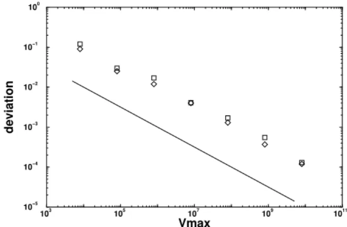
This dynamic rule was applied according to a previously planned visit profile, equivalent to Fig. 10, covering contin-uouslyan entire interval of temperatures within a uniform accuracy. For a32×32lattice, the exact partition function is available [19], and we can compute the deviations obtained for the specific heat, for instance. At the peak, in particular, these deviations are the largest, shown in Fig. 11 as a func-tion of the statistics. Different symbols correspond to the possible values∆E = 1or 2, fixed for the energy jump in the broad histogram equation.
103 105 107 109 1011
Vmax
10−5 10−4 10−3 10−2 10−1 100
deviation
Figure 11. Deviations relative to exact values of the specific heat peak,32×32Ising model. The line shows1/√Vmax, in order
to compare the slopes. Diamonds correspond to∆E = 1, and squares to∆E= 2.
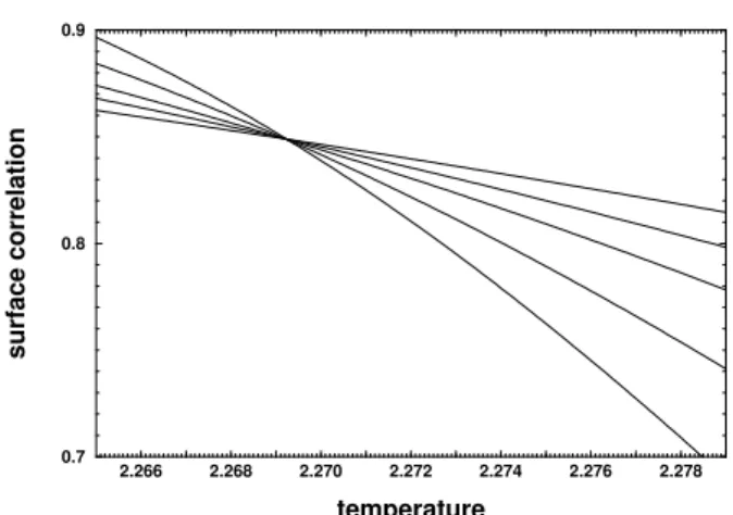
determines the productr =SiSj, and perform the average of this quantity over allLpossible pairs of parallel lines dis-tantL/2from each other (rows and columns). The quoted surface correlation is the canonical average< r >T of this quantity.
2.15 2.25 2.35
temperature
0.0 0.5 1.0
surface correlation
32
126
Figure 12. Surface correlation function for theL×Lsquare lattice Ising model,L = 32, 46, 62, 90 and 126. For larger and larger lattices, these plots approach the step function defined by the bold straight lines plus the circle.
In the thermodynamic limitL → ∞, this quantity is a kind of order parameter, Fig. 12, vanishing above the critical temperatureTc. For increasing lattice sizes, it approaches a step function: < r >T = 1belowTc;< r >T = r∗ at
Tc, wherer∗is a universal value; and< r >T = 0above
Tc. The distinguishing feature of< r >T, compared with the usual order parameter (the magnetisation< m >T) is its constant behaviourbelowthe critical temperature. On one hand,< m >T ∼ (Tc−T)βnear and belowTc. On the other hand, also belowTcone has< r >T = 1, hence, instead ofβ, the corresponding exponentvanishes[5]. For finite systems, considering the finite size scaling hypothesis, this comparison can be better appreciated within the gener-alised homogeneous forms
m[λ1/ν(T−Tc), λL−1] =λ−φm m(T−T
c, L−1) ,
where the alternative notation< m >T = m(T−Tc, L−1) is adopted, and
r[λ1/ν(T−Tc), λL−1] =λ−φr r(T−T
c, L−1) ,
where< r >T = r(T−Tc, L−1).
2.266 2.268 2.270 2.272 2.274 2.276 2.278
temperature
0.7 0.8 0.9
surface correlation
Figure 13. A zoom performed on the previous plot.
These forms are asymptotically valid for large L and near Tc, where λ is an arbitrary length. By choosing
λ = |T −Tc|−ν and taking the limitL → ∞, one finds
φm = −β/νandφr = 0. On the other hand, by choos-ingλ = Land tuning the system exactly atTc, one finds
< m >T ∼ Lφm =L−β/νand< r >T ∼ Lφr =L0. At
Tcand for largeL,< r >T becomes size independent, i.e.
< r >T = r∗. A possible approach to find the critical tem-peratureTcis by plotting< r >TagainstTfor two different lattice sizes, and finding the crossing of both curves. Fig. 12 shows< r >T for 5 different lattice sizes, obtained by the broad histogram method. The maximum number Vmax of sampled states per energy level was8×109forL= 32and 46, and8×108forL= 62, 90 and 126.
2.266 2.268 2.270 2.272 2.274 2.276 2.278
temperature
0.60 0.62 0.64
Binder cumulant
Figure 14. The Binder cumulant within the same zoom.
The so-called Binder cumulant< u >T[4] also presents zero anomalous dimension. It was very often used in or-der to find critical temperatures of many systems, following the same idea of finding the crossing between two curves
cumulant obtained from the same computer runs, thus with the same accuracy. The surface correlation function seems to work better than the Binder cumulant. The reason for that may be traced from the scaling behaviour on three distinct points, namelyT = 0,T → ∞and, of course, the critical pointT =Tc. The system is invariant under scaling trans-formations not only at the critical point, but also forT = 0 andT → ∞. Thus, besides the thermal exponentνand the magnetic exponentδ, both describing the critical behaviour nearTc, there are other (non-critical) exponents related to the lattice dimensionality which describes the behaviour of the system under scaling transformation nearT = 0 and nearT → ∞. By construction, both the Binder cumulant
< u >T and the surface correlation function< r >T re-spect the correct critical behaviour nearTc. However, only
< r >T, not < u >T, does the same near T = 0 and
T → ∞ [5]. Thus, being forced to obey the correct be-haviours in three different points along theT axis,< r >T has less freedom to deviate from the correctL → ∞ be-haviour, even for small system sizes.
4
Self-Organized Criticality
4.1
Introduction
Self-organized criticality (abbreviated as SOC from here on) describes a large and varied body of phenomenological data and theoretical work. Because its current meaning has evolved far from any initial precise meaning the term may have had, we will in these notes adhere to a broad character-ization, if only for pedagogical purposes.
The original motivation for SOC came from recursive mathematics. Iterated maps have been show to generate fascinating images -fractals - which are now in common usage, both in the sciences and in popular culture. Some of these patterns looked very similar to naturally occurring ones, such as river erosion patterns, plant and leaf structure, and geological landscapes, to name but a few. The question about which kinds of dynamical mechanisms would be re-quired to create such patterns in nature is, thus, unavoidable. One would hope, in addition, this mechanisms to be fairly simple: very little would be gained in our understanding if they were as complex as the patterns they generate.
The breakthrough in this field can undoubtedly be at-tributed to a seminal paper by Back, Tang, and Wiesenfeld (BTW) in 1987 [20], that opened the path to a variety of computational models that show SOC behavior. These mod-els are also successful in demonstrating the possibility of generating complex and coherent structures from very sim-ple dynamical rules. A key feature of these models is that they are capable of generating spatially distributed patterns of a fractal nature without requiring long-range interactions in their dynamics: the long-range correlations “emerge” from short-range interaction rules. Another key feature of these models is the fact that they converge to “absorbing” configurations exhibiting long-range coherence even having not started at one. This convergence does not require the tuning of any external parameter, and thus these models are said to be “self-organized”.
Criticality is a notion that comes from thermodynamics. In general, thermodynamic systems become more ordered and decrease their symmetry as the temperature is lowered. Cohesion overcomes entropy and thermal motion, and struc-tured patterns begin to emerge. Thermodynamic systems can exist in a number of phases, corresponding to differ-ent orderings and symmetries. Phase transitions that take place under the condition of thermal equilibrium, for which temperature is a well-defined quantity and the free energy is minimized, are well understood. These equilibrium sys-tems are ergodic and have had time to settle into their most probable configuration, allowing simplifying statistical as-sumptions to be made. Although most phase transitions in nature are discontinuous, in the sense that at least one re-sponse function - a first-order derivative of the free energy - suffers a discontinuous jump at the transition point, some systems may show a critical point at which this disconti-nuity does not happens. As a system approaches a critical point from high temperatures, it begins to organize itself at a microscopic level. Near but not exactly at the critical point, correlations have an exponential decay - as an exam-ple for the Ising model, whereS(~r) is the spin, the spin-spin correlation has the typical behavior < S(~r)S(0) >τ −< S(0)>τ2 ∼ exp(−r/ξ)r−A, whereξis called the correlation length. Close to the critical point, large struc-tural fluctuations appear, yet they come from local interac-tions. These fluctuations result in the disappearance of a characteristic scale in the system at the critical point - in the example above, the same spin-spin correlation function is now< S(~r)S(0) >τ −< S(0)>τ2 ∼ r−A, which amounts to havingξ→ ∞in the former equation. It is fair to say that the lack of a characteristic scale is the hallmark of a critical process. This behavior is remarkably general and independent of the system’s dynamics.
The kind of structures that SOC aspires to explain look like equilibrium thermodynamic systems near their critical point. Typical SOC systems, however, are not in equilibrium with their surroundings, but have instead non-trivial interac-tions with them. In addition, SOC systems do not require the tuning of an external control parameter, such as temperature, to exhibit critical behavior. They tune themselves to a point at which critical-type behavior occurs. This critical behav-ior is the bridge between fractal structures and thermody-namics. Fractal structures appear the same at all size scales, hence they have no characteristic scale, just as the fluctua-tions near an equilibrium phase transition at a critical point. It is then logically compelling to seek a dynamical explana-tion of fractal structures in terms of thermodynamic critical-ity. A proper understanding of SOC requires an extension of the notion of critical behavior to non-equilibrium ther-modynamical systems and hence an extension of the tools required to describe such systems.
generated from an initial element by an iterated map implies that the number of elementsN(s)has a power-law depen-dence on their size s. This is precisely what we mean by scale invariance, sincef(x) =xA
→f(kx)/f(x) =kA . The main hypothesis contained in the work of BTW is that a dynamical system with many interacting elements, un-der very general conditions, may self-organize, or self-tune, into a statistically stationary state with a complex structure. In this state there are no characteristic scales of time and space controlling the time evolution, and the dynamical re-sponses are complex, with statistical properties described by power-laws. Systems with very different microscopic dynamics can present power-law responses with the same exponents, in a non-equilibrium version of Wilson’s idea of universality: These self-organized states have properties similar to those exhibited by equilibrium systems at their critical point.
This mechanism is a candidate to be the long sought dy-namical explanation for the ubiquity in nature of complex space-time structures. A list of phenomena that could ex-hibit SOC behavior include the avalanche-response of sand piles, earthquakes, landslides, forest fires, the motion of magnetic field lines in superconductors and stellar atmo-spheres, the dynamics of magnetic domains, of interface growth, and punctuated equilibrium in biological evolution. What are the ingredients that lead a driven dynamical system to a SOC state? From the analysis of the computa-tional models mentioned at the beginning of this section, a key feature is a large separation between the time scales of the driving and the relaxation processes. This can be ensured by the existence of a threshold that separates them. As an ex-ample, let us consider the physics of driven rough interfaces, which is believed to be one of the main earthquake source processes. This connection will be analyzed in more detail in the next section, but for our present purposes it is enough to mention that the separation of time scales is in this case provided by static friction, which has to be overcome by the increasing stress between the two sides of a geological fault. A SOC state is thus a statistically stationary state, said to be “marginally stable”, sharing with thermodynamical critical states the property of space-time scale invariance, with algebraically decaying correlation functions. It is per-haps best seen as a collection of metastable states, in the thermodynamical sense. The system is driven across phase space, spending some time at the neighborhood of each of its metastable states, and moving between these states after some large avalanche of relaxation events.
The original goal of BTW was to provide an explanation for the frequent occurrence in nature of fractal space and time patterns. The latter are usually referred to as one-over-f (1/f) noise, indicating the scale invariance of the power spectrum. The SOC dynamical answer to this quest goes as follows: In driven extended threshold systems, the response
(signal) evolves along a connected path of regions above the
threshold. Noise, generated either by the initial configura-tion or built in the dynamics, creates random connected net-works, which are modified and correlated by the intrinsic dynamics of relaxation. The result is a complex patchwork of dynamically connected regions, with a sparse geometry
resembling that of percolation clusters. If the activated re-gion consists of fractals of different sizes, the energy release and the time duration of the induced relaxation events that travel through this network can vary enormously.
4.2
Characterization of the SOC state
The nature of the state is best described by the system’s response to an external perturbation. Non-critical systems present a simple behavior: The response time and the de-cay length have characteristic sizes, their distribution is nar-row and well described by their first moment (average re-sponse). In critical systems, on the other hand, the same perturbation can generate wildly varying responses, depend-ing on where and when it is applied. The statistical distri-butions that describe the responses have the typical func-tional form P(s) ∼ s−τ and Q(t) ∼ t−α. These dis-tributions have a lower cutoff s1 and t1, defined by the scale of the microscopic constituents of the system. For finite systems of linear size L, the distributions present a crossover, from a certain scale up, to a functional form such asP(s)∼exp(−s/s2),s > s2. For a genuine critical state, one must haves2 ∼ Lw,w > 0. If the exponent of the distribution isω < 2, it has no mean in the thermodynamic limit; if it is<3, its second moment and width diverge.
The temporal fluctuations are characterized by a 1/f
noise. This is a rather imprecise label used to describe the nature of certain types of temporal correlations. If the response of a physical system is a time-dependent signal
N(τ), the temporal correlation functionG(τ), defined by
G(τ) =< N(τ0)N(τ0+τ)>τ0 −< N(τ0)>τ0 2
, (1) describes how the value of the signal at some instant in timeN(τ0)has a statistical significance in its value at some later timeN(τ0+τ). If there is no statistical correlation,
G(τ) = 0. The rate of decrease ofG(τ), fromG(0)to0, measures the duration of the correlation, and is related to memory effects in the signal.
The power spectrum of the signalN(τ)is related to its Fourier transform
S(f) = lim T→∞
1 2T
¯ ¯ ¯
Z T
−T
N(τ)exp(2iπf τ)dτ¯¯ ¯
2 (2)
For a stationary process,
S(f) = 2 Z ∞
0
G(τ)cos(2πf τ)dτ (3) and temporal correlations may be discussed in terms of the power spectrum.
It is interesting to note that the sandpile model proposed as an archetypical SOC system by BTW, even though show-ing long range time correlations, doesnotpresent1/fnoise, despite the claims to the contrary originally made by its pro-ponents.
Let us now discuss the spatial correlation function. For a system described by a dynamical variable which is a field
n(r,t), such as the local density (or the local magnetization)
for fluid (or magnetic) systems this function is
G(r) =< n(r0+r)n(r0)>r0−< n(r0)>r0
2 (4) where the brackets indicate thermal and positional averages. IfT 6= Tc,G(r) ∼ exp(−r/ξ), whereξis the corre-lation length. IfT → Tc,ξ ∼| T −Tc |−ν. AtT = Tc,
G(r)∼r−η. The divergence ofξindicates the absence of a characteristic length scale and leads to spatial scale invari-ance.
4.3
Systems that exhibit SOC
Model systems have been shown to fulfill the SOC char-acterization. But this is not enough for the SOC program: one should examine real physical systems and identify ex-perimentally SOC behavior, if this concept is to be at all significant to our understanding of nature. In the experi-ments, one usually collects data about the statistical size dis-tribution of the dynamical responses, arising from the relax-ation avalanches. But what should we look for in this data? One possibility, raised by our previous comments, would be to measure time-dependent dynamical quantities and com-pute their power spectrum. Unfortunately, it turns out that a power spectrum of the form∼ 1/fβ,β ≃ 1, is a neces-sary, but not sufficient condition for critical behavior, thus for SOC. One has also to identify the presence of spatial fractals in order to be able to characterize a real-life SOC system.
Experiments measuring the avalanche signals of sandpile-like systems, which mimic the original BTW model, failed in all but one case to show evidence of SOC behavior. Typically, in these systems, sand is slowly added to a pile. In one experiment, for example, this pile had a circular base, and was set on top of a scale, which could monitor fluctuations of the total mass. Small piles did show scale invariance. As the diameter of the base increases, a crossover to an oscillatory behavior is observed: Small avalanches in real sandpiles do show a behavior consis-tent with SOC, which disappears when the mean avalanche size increases. In order to investigate inertial effects that could be responsible for the destruction of the incipient SOC state, experiments were performed with one-dimensional rice piles, with grains differing by their aspect ratio. In this case, the signal observed was the potential energy release. For small and nearly spherical grains (aspect ratio∼1), the distribution of event sizes is a stretched exponential of the formP(E)∼exp[(−E/E0)γ]. For elongated grains, with a larger aspect ratio, this distribution, obtained through a finite-size-scaling of the data, isP(E)∼E−α, with no
fi-nite size cutoff [21]. This scale invariance is consistent with SOC behavior.
Another strong candidate for SOC behavior in the real world is the avalanche response of geological plate tecton-ics, the earthquakes. Earthquakes result from the tectonic motion of the plates on the lithosfere of our planet. This mo-tion, driven by convection currents in the deep mantle, gen-erates increasing stresses along plate interfaces, since slid-ing is avoided by static friction. Plate speeds beslid-ing typically in the range of a few cm/year, which amounts to a slow drive, and the threshold dynamics implicit in friction, are the two ingredients that can generate SOC for this planetary system. In fact, the distribution of earthquake occurrence has been shown to obey Gutenberg-Richter’s law: it is a broad dis-tribution, withP(E) ∼ E−B, B ∼ 1.8−2.2, and some geographical dependence on the exponent. There is some controversy in the geophysical literature about the validity of this statistical description, and some claim that a charac-teristic, periodic regime can be observed for some faults, for events at the far end (large size) of the distribution.
The cascades of species extinctions that result from bi-ological evolution are other phenomena for which claims of SOC behavior have been stated. Paleontological evidence, though sparse and debatable, seems to point towards a de-scription of a system in “punctuated equilibrium”, a term that invokes long periods of relative quiescence (“equilib-rium”) interrupted (“punctuated”) by short, in the time scale of evolution, periods of frenetic activity, in which large num-bers of species disappear. In contrast to a gradual process of species extinction and creation, such a view is underlined by an understanding of extinction as a result of fluctuation in environment pressure, rather than to species obsolescence. As a species disappear because of its poor fitness to the changing environment, the effects will propagate through a variable-length network of neighboring species in the food chain, in an avalanche of extinctions. The distribution of avalanche sizes appear, from the known evidence, to exhibit scale invariance, thus the already mentioned claim for SOC behavior.