Removing low-frequency artefacts from Datawell DWR-G4 wave buoy measurements

(1)

GID

5, 363–383, 2015

Removing low-frequency artefacts from Datawell DWR-G4

J.-V. Björkqvist et al.

Title Page

Abstract Introduction

Conclusions References

Tables Figures

◭ ◮

Back Close

Full Screen / Esc

Printer-friendly Version Interactive Discussion

Discussion

P

a

per

|

Discussion

P

a

per

|

Discussion

P

a

per

|

Discussion

P

a

per

|

Geosci. Instrum. Method. Data Syst. Discuss., 5, 363–383, 2015 www.geosci-instrum-method-data-syst-discuss.net/5/363/2015/ doi:10.5194/gid-5-363-2015

This discussion paper is/has been under review for the journal Geoscientific Instrumentation, Methods and Data Systems (GI). Please refer to the corresponding final paper in GI if available.

Removing low-frequency artefacts from

Datawell DWR-G4 wave buoy

measurements

J.-V. Björkqvist, H. Pettersson, L. Laakso, K. K. Kahma, H. Jokinen, and P. Kosloff

Finnish Meteorological Institute, Helsinki, Finland

Received: 11 September 2015 – Accepted: 22 October 2015 – Published: 3 November 2015

Correspondence to: J.-V. Björkqvist (jan-victor.bjorkqvist@fmi.fi)

(2)

GID

5, 363–383, 2015

Title Page

Tables Figures

◭ ◮

Back Close

Full Screen / Esc

Discussion

P

a

per

|

Discussion

P

a

per

|

Discussion

P

a

per

|

Discussion

P

a

per

|

Abstract

In this study we describe a previously unreported error in the vertical displacement time series made with GPS-based Datawell DWR-G4 wave buoys and introduce a simple method to correct the resulting wave spectra. The artefact in the time series is found to resemble a sawtooth wave, which produces an erroneous trend following

5

anf−2_{power law in frequency space. The correction method quantifies the amount of}

erroneous trend below a certain maximum frequency and removes the spurious energy

from all frequencies assuming the above mentioned f−2 _{power law. The presented}

correction method is validated against an experimental field test and its impact on the measured significant wave height is quantified. The method’s sensitivity to the choice

10

of the maximum frequency is also briefly discussed.

1 Introduction

Surface wind waves are an important factor for the safety and e_fficiency of marine

traffic, sea-borne operations and coastal structures. Short-term observations are well

suited to map the wave field and to support wave model development, especially at

15

complex shorelines. Currently the large wave buoys utilising accelerometers to mea-sure the pitch, heave and roll of the buoy are considered highly reliably instruments for

operational measurements. Nevertheless, there also exists several different

technolo-gies that use a GPS-receiver to measure the displacement of the wave buoy, which

have all been proven to be sufficiently accurate in a majority of situations (Herbers

20

et al., 2012). Especially the technique using the Doppler shift of the GPS-signal to measure the velocity of the wave buoy have been shown to produce excellent results when compared to an accelerometer based Datawell Directional Waverider (“DWR”) (de Vries et al., 2003; Jeans et al., 2003).

The small size of the GPS-receiver enables the construction of smaller and more

25

(3)

GID

5, 363–383, 2015

Title Page

Tables Figures

◭ ◮

Back Close

Full Screen / Esc

Discussion

P

a

per

|

Discussion

P

a

per

|

Discussion

P

a

per

|

Discussion

P

a

per

|

According to our experience these smaller buoys are practical and cost efficient,

espe-cially for short measurements (e.g. Tuomi et al., 2014) where they can be moored or deployed as floating devices.

In this paper we describe an observed error reading in the G4 measurements, sug-gest an easy and automated corrective method and discuss the accuracy and

limita-5

tions of the correction based on experiments.

2 The artefact

Although the overall accuracy of the Datawell G4 is not in question, we have observed anomalous behaviour in the vertical displacement time series calculated on board

sev-eral different G4 wave buoys over the course of almost a decade. The artefact is large

10

enough to affect the reliability of even robust wave parameters, such as the

signifi-cant wave height, if no correction is applied. The sawtooth like artefact in the time series (Fig. 1) can not be explained by the mooring (e.g. Ashton and Johanning, 2015), as we have also observed similar behaviour with free floating buoys during measure-ment campaigns and completely stationary buoys during routine testing. We also rule

15

out instrument failure, since the anomaly has been observed with several individual buoys. We suspect that the source of the artefact might be linked to disturbances in the propagation of the GPS-signal that are caused by atmospheric conditions. Even if the receiving unit is functioning properly, any disturbances in the propagation of the sig-nal could lead to an incorrect determination of the velocity of the wave buoy, since the

20

(4)

GID

5, 363–383, 2015

Title Page

Tables Figures

◭ ◮

Back Close

Full Screen / Esc

Discussion

P

a

per

|

Discussion

P

a

per

|

Discussion

P

a

per

|

Discussion

P

a

per

|

3 The wave spectrum and the correction method

3.1 The wave spectrum

The irregular nature and frequent occurrence of the anomaly described in Sect. 2

makes manual cleaning both difficult and extremely time consuming. However, the

main interest of researchers is usually not the vertical displacement of the buoy, but

5

rather the wave spectrum, which describes the wave field in the frequency domain. Es-pecially the parameters derived from the 1-D spectrum, e.g. the significant wave height and wave periods are extensively used both for operational and for research purposes. The 1-D wave spectrum is the power density spectrum of the vertical displacement. Theoretically it is defined as the Fourier transform of the autocovariance function of the

10

vertical displacement, but in practice it is usually calculated directly form the vertical displacement by using the Fast Fourier Transform (FFT) (see e.g. Bendat and Piersol, 2010). All the wave spectra in this study are the ones calculated on board the wave buoys by taking the Fourier transform piecewise from the time series, but the correction technique we propose is not dependant on the method used to calculate the wave

15

spectrum. For a more detailed description of the method used on board the buoys the reader is referred to the Datawell manual (Datawell BV, 2014).

A schematic illustration of the frequency responses of the relevant signals is shown in

Fig. 2. The power density spectrum of a sawtooth wave follows anf−2_{frequency power}

law, which is not limited by any upper frequency. Solutions depending on discarding all

20

data from the spectra below a cut-off frequency will therefore not be sufficient, even

though it has previously been used to remove erroneous low-frequency data of a dif-ferent type (Joodaki et al., 2013).

The observed error reading in Fig. 1 has the shape of a sawtooth wave. The correc-tion method presented in this paper will therefore be based on the known frequency

25

(5)

GID

5, 363–383, 2015

Title Page

Tables Figures

◭ ◮

Back Close

Full Screen / Esc

Discussion

P

a

per

|

Discussion

P

a

per

|

Discussion

P

a

per

|

Discussion

P

a

per

|

3.2 The correction method

To quantify the amount of spurious energy we will first need to determine a frequency interval that we can assume to contain pure erroneous trend. As a first guess for the upper limit we took 0.07 Hz. This choice was based on our long experience that there is practically no physically meaningful wave data below that frequency in the Baltic Sea

5

(e.g. Kahma, 1981; Kahma et al., 2003; Pettersson, 2004; Tuomi, 2008; Tuomi et al., 2011). For the purpose of our calculations we can therefore assume that frequencies below 0.07 Hz contain only pure erroneous trend. The choice of frequency interval for

e.g. a different geographical location will have to be made based on the knowledge of

the local wave field. The effect the chosen maximum frequency has on our results is

10

further discussed in Sect. 5.

Because of the underlying f−2 _{power law the erroneous trend will have a constant}

value if the spectrum is scaled by a factor off2. We will then calculate the mean value of

the scaled trend from frequencies below 0.07 Hz and remove it from the entire spectrum prior to de-scaling. A schematic picture of the de-trending process is shown in Fig. 3.

15

In practice the trend will not always be smooth. The variations around the mean value may cause small positive and negative residuals even below the chosen maximum frequency of 0.07 Hz. As an additional step, we will remove any residuals below 0.07 Hz (usually very small) and set possible negative values to zero (because the original spectral file is always strictly non-negative). The first step is mostly cosmetic and the

20

latter practical. We want to stress that the real correction of the spectrum is made by the removing of the mean trend.

4 Experimental

We at the Finnish Meteorological Institute1(FMI) have observed waves in the Baltic Sea

since the 1970s both campaign-based (e.g. Kahma, 1981; Pettersson, 2004; Tuomi

25

1

(6)

GID

5, 363–383, 2015

Title Page

Tables Figures

◭ ◮

Back Close

Full Screen / Esc

Discussion

P

a

per

|

Discussion

P

a

per

|

Discussion

P

a

per

|

Discussion

P

a

per

|

et al., 2014) and operationally (e.g. Pettersson and Jönsson, 2004; Tuomi, 2008). The measurements have been conducted with various instruments including wave buoys,

Acoustic Doppler Current Profilers (ADCP) and wave staffs. Our operational

measure-ments are made with wave buoys equipped with accelerometer based sensors, but we have also used GPS-based wave buoys for additional shorter measurements since

5

2006.

To test the correction method described in Sect. 3 we deployed a GPS-based Datawell DWR-G4 (henceforth, “the G4”) in close proximity to FMI’s operational ac-celerometer based Directional Waverider (“the DWR”) in the centre of the Gulf of Fin-land (Fig. 4). The measurement period for the G4 was 4–20 May 2015, during which

10

time the significant wave height measured by the DWR ranged from 0.1 to 2.9 m. Both wave buoys use a 0.78 s sampling time to measure the 1600 s time series from which they calculate the wave spectra every half hour. The spectra from both buoys have a frequency range of 0.025–0.580 Hz with a resolution of 0.01 Hz (0.005 Hz for frequencies under 0.1 Hz).

15

The significant wave height is defined asH_s₌₄√m₀_{, where}m₀_{is the zeroth-moment}

(i.e. the integral) of the wave spectrum. The integral of the wave spectrum is also the variance of the vertical displacement time series.

5 Results

The variance density (m2Hz−1_{) of each frequency bin from the G4 wave buoy was}

20

compared to those of the DWR for the whole dataset. Figure 5 shows the bias of the original and corrected G4 spectra compared to the reference data from the DWR. We

can see that the original G4 data has a positive bias following the expectedf−2_power

law, which is no longer visible after the correction. The correction method applied to the, presumably correct, DWR spectra resulted in only negligible changes (not shown).

25

(7)

GID

5, 363–383, 2015

Title Page

Tables Figures

◭ ◮

Back Close

Full Screen / Esc

Discussion

P

a

per

|

Discussion

P

a

per

|

Discussion

P

a

per

|

Discussion

P

a

per

|

anomaly in our field data we plotted the difference in significant wave height from the

G4 buoy before and after the use of the correction method in a logarithmic histogram

(Fig. 6). The relative value is defined as the difference between the original and

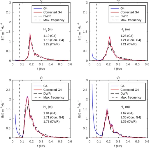
cor-rected significant wave height normalised by the original significant wave height. Four situations with an increasing amount of erroneous trend is shown in Fig. 7.

5

The first case (a) illustrates that the method does not interfere with an uncorrupted spectrum. In the three following cases the erroneous trend continues above the maxi-mum frequency used to quantify the spurious energy (0.07 Hz), but even these higher frequencies are corrected as a comparison to the DWR spectra reveals.

In addition to errors in the significant wave height the artefact will also lead to

unphys-10

ical values if the peak period (i.e. the period containing the most energy) is calculated for situations resembling that of Fig. 7d. This must be taken into account especially in operational applications, but the data need not be discarded if a proper automated correction method is used.

Because of the small size of the Baltic Sea, we were able to use a relatively high

15

maximum frequency of 0.07 Hz (i.e. 14 s wave period) as an initial guess for an appro-priate value. However, one cannot generally assume that there is no physically relevant wave data below 0.07 Hz, which calls for a lower upper limit when quantifying the trend. To test the sensitivity of the method we repeated the calculations using a maximum fre-quency of 0.04 Hz (i.e. 25 s wave period).

20

The results in Table 1 show the difference in significant wave height between the G4

and the DWR wave buoys when using the different frequency intervals. We calculated

the values using only the data when erroneous trend was observed, which we defined somewhat arbitrarily as cases when the correction of the significant wave height to the G4 wave buoy was at least 0.1 m. The results show that the proposed method is

25

insensitive to the choice of the maximum frequency. This is easily explained by the fact that the level of the trend is equally well defined below 0.04 Hz (Fig. 8b).

To better illustrate even the small differences between the original and corrected

(8)

GID

5, 363–383, 2015

Title Page

Tables Figures

◭ ◮

Back Close

Full Screen / Esc

Discussion

P

a

per

|

Discussion

P

a

per

|

Discussion

P

a

per

|

Discussion

P

a

per

|

A trend following anf−2 _{power law should be linear in a logarithmic plot, which is}

in-deed the case. The figure also illustrates that a slight overcorrection is possible for the highest frequencies (0.40–0.58 Hz), where the trend becomes the same order of magnitude as the spectrum. This can be due to other small low-frequency errors that contribute to the spectrum below 0.07 Hz, which in turn will make the correction slightly

5

too large. However, this possible overcorrection is inconsequential for the calculation of any basic parameters, such as the significant wave height. Even though we recom-mend the corrected data to be carefully checked when used in advanced wave studies, the method presented in this paper is suitable to be implemented as an automated approach for e.g. operational applications.

10

6 Conclusions

In this paper we introduce a simple automated method to correct Datawell DWR-G4 data for an error observed in the lower frequencies. This error is caused by a sawtooth

like artefact in the time domain and thus follow an f−2 _{power law in the frequency}

domain (Figs. 1 and 2). We have concluded that the artefact in the time domain is

15

caused by the use of the Doppler shift technology, but are not aware of any previous reports of this kind of behaviour.

The basic idea of the method is to calculate the level of the erroneous trend from the frequency bins we know to lack physical relevant information (we used 0.07 Hz as an upper limit for the Baltic Sea) and then remove it for the whole frequency range (see

20

Fig. 3 for a schematic overview of the method).

We compared the original and corrected spectra to reference spectra made with an accelerometer based Datawell Directional Waverider moored 900 m away. The cor-rected spectra match the reference spectra better than the original ones for the lower frequencies. In addition, the excess erroneous energy in the spectra is removed also

25

(9)

GID

5, 363–383, 2015

Title Page

Tables Figures

◭ ◮

Back Close

Full Screen / Esc

Discussion

P

a

per

|

Discussion

P

a

per

|

Discussion

P

a

per

|

Discussion

P

a

per

|

shows that the power law method increases the accuracy of the observations even if only integrated parameters, such as e.g. significant wave height, are considered.

The results presented in Table 1 show that the method produces the same results if the level of the erroneous trend is quantified only below 0.04 Hz. This robustness

increases the usability of the correction method for different physical and geographical

5

conditions.

Although the correction is generally concentrated to the low-frequency part of the spectrum, there is a possibility of a small overcorrection of the high-frequency tail

(>_{0.4 Hz) (Fig. 9). Luckily, these minor di}_ff_{erences are not important for basic}

appli-cations that uses only integrated parameters. Nonetheless, the corrected data should

10

be analysed if they are to be used for more advanced wave research.

Appendix

A Simple MATLAB code for correcting data from Datawell G4 wave buoys.

% Remove trend from wave spectrum measured by Datawell % DWR-G4 wave buoys

15

%

% function S_DT=detrend_wavespec(f,S,f_max) % ---% f is the frequency [vector]

% S is the spectral density [vector]

20

% f_max is the maximum frequency [double] % ---% Borkqvist et al. (2015)

function S_DT=detrend_wavespec(f,S,f_max)

25

(10)

GID

5, 363–383, 2015

Title Page

Tables Figures

◭ ◮

Back Close

Full Screen / Esc

Discussion

P

a

per

|

Discussion

P

a

per

|

Discussion

P

a

per

|

Discussion

P

a

per

|

bin_max=find(f<=f_max,1,’last’); % Select the bins used to % calculate the trend

Trend=mean(S_scaled(1:bin_max)); % Calculate mean scaled trend S_scaled=S_scaled-Trend; % Remove mean scaled trend

S_scaled(1:bin_max)=0; % These freq. bins did not contain any

5

% real information

S_scaled=max(S_scaled,0); % Force to positive values

S_DT=S_scaled./f.^2; % Return the de-scaled spectrum

Data availability

10

The spectral files of both the wave buoys for the study period and the MATLAB code found in Appendix A are available as Supplement.

The Supplement related to this article is available online at doi:10.5194/-15-363-2015-supplement.

Acknowledgements. We are grateful to Senior Scientist Kristian Spilling from the Finnish Envi-15

ronment Institute for arranging the time for our measurements during his cruise on RVAranda

on such a short notice.

References

Ashton, I. G. C. and Johanning, L.: On errors in low frequency wave measurements from wave buoys, Ocean Eng., 95, 11–22, doi:10.1016/j.oceaneng.2014.11.033, 2015. 365

20

Bendat, J. S. and Piersol, A. G.: Random Data: Analysis and Measurement Procedures, 4th Edn., Wiley Series in Probability and Statistics, Hoboken, New Jersey, 2010. 366 Datawell BV: Datawell Waverider Manual DWR4, available at: http://datawell.xcess-5.

xec.nl/Portals/0/Documents/Manuals/datawell_manual_dwr4_2014-11-10.pdf (last access: 10 September 2015), 2014. 366

(11)

GID

5, 363–383, 2015

Title Page

Tables Figures

◭ ◮

Back Close

Full Screen / Esc

Discussion

P

a

per

|

Discussion

P

a

per

|

Discussion

P

a

per

|

Discussion

P

a

per

|

de Vries, J. J., Waldron, J., and Cunningham, V.: Field tests of the New Datawell DWR-G GPS wave buoy, Sea Technol., 44, 50–55, 2003. 364

Herbers, T. H. C., Jessen, P. F., Janssen, T. T., Colbert, D. B., and MacMahan, J. H.: Observ-ing ocean surface waves with GPS-tracked buoys, J. Atmos. Ocean. Tech., 29, 944–959, doi:10.1175/JTECH-D-11-00128.1, 2012. 364

5

Jeans, G., Bellamy, I., de Vries, J. J., and van Weer, P.: Sea trial of the new datawell GPS directional waverider, in: Proceeding of the IEEE/OES Seventh Working Conference, San Diego, CA, USA, 145–147, doi:10.1109/CCM.2003.1194302, 2003. 364

Joodaki, G., Nahavandchi, H., and Cheng, K.: Ocean wave measurements using GPS buoys, J. Geodet. Sci., 3, 163–172, doi:10.2478/jogs-2013-0023, 2013. 366

10

Kahma, K. K.: A study of the growth of the wave spectrum with fetch, J. Phys. Oceanogr., 11, 1504–1515, doi:10.1175/1520-0485(1981)011<1503:ASOTGO>2.0.CO;2, 1981. 367 Kahma, K. K., Pettersson, H., and Tuomi, L.: Scatter diagram wave statistics from the Northern

Baltic Sea, Rep. Ser. Finnish Inst. Mar. Res., 49, 15–32, 2003. 367

Pettersson, H.: Wave Growth in a Narrow Bay, Finnish Institute of Marine Research – Contribu-15

tions, Helsinki, Finland, 1–33, 2004. 367

Pettersson, H. and Jönsson, A.: Wave climate in the northern Baltic Sea in 2004, available at: http://www.helcom.fi/baltic-sea-trends/environment-fact-sheets/ (last access: 10 Septem-ber 2015), 2004. 368

Tuomi, L.: The accuracy of FIMR wave forecasts in 2002–2005, Rep. Ser. Finnish Inst. Mar. 20

Res., 63, 7–17, 2008. 367, 368

Tuomi, L., Kahma, K. K., and Pettersson, H.: Wave hindcast statistics in the seasonally ice-covered Baltic Sea, Boreal Environ. Res., 16, 451–472, 2011. 367

Tuomi, L., Pettersson, H., Fortelius, C., Tikka, K., Björkqvist, J.-V., and Kahma, K. K.: Wave modelling in archipelagos, Coast. Eng., 83, 205–220, doi:10.1016/j.coastaleng.2013.10.011, 25

(12)

GID

5, 363–383, 2015

Title Page

Tables Figures

◭ ◮

Back Close

Full Screen / Esc

Discussion

P

a

per

|

Discussion

P

a

per

|

Discussion

P

a

per

|

Discussion

P

a

per

|

Table 1.Mean and extreme difference in significant wave height of the G4 wave buoy when compared to the DWR wave buoy. The significant wave height is calculated for both the entire frequency range and for the low-frequency part of the spectra only. Two corrections are made using different maximum frequencies to quantify the erroneous energy. Values are calculated from data where erroneous energy was present (i.e. the correction by the method was at least 0.1 m).

∆H_s(<0.1 Hz) ∆H_s

G4 vs. DWR mean (m) extreme (m) mean (m) extreme (m)

Uncorrected 0.8 1.8 0.2 0.7

Correction usingf <0.07 Hz 0.0 0.2 −0.1 −0.5

(13)

GID

5, 363–383, 2015

Title Page

Tables Figures

◭ ◮

Back Close

Full Screen / Esc

Discussion

P

a

per

|

Discussion

P

a

per

|

Discussion

P

a

per

|

Discussion

P

a

per

|

0 200 400 600 800 1000 1200 1400 1600 1800

−2 −1 0 1 2

t (s)

z (m)

0 200 400 600 800 1000 1200 1400 1600 1800

−2 −1 0 1 2

t (s)

z (m)

(14)

GID

5, 363–383, 2015

Title Page

Tables Figures

◭ ◮

Back Close

Full Screen / Esc

Discussion

P

a

per

|

Discussion

P

a

per

|

Discussion

P

a

per

|

Discussion

P

a

per

|

0 100 200 300 400 500 −2

−1 0 1 2

Time (s)

Vertical displacement (m)

a)

0 0.1 0.2 0.3 0.4

0 1 2 3 4 5

Frequency (Hz)

Variance density (m

2Hz

−1

b)

0 100 200 300 400 500 −2

−1 0 1 2

Time (s)

c)

0 0.1 0.2 0.3 0.4

0 1 2 3 4 5

Frequency (Hz)

Variance density (m

2Hz

−1

) d)

0 100 200 300 400 500 −2

−1 0 1 2

Time (s)

e)

0 0.1 0.2 0.3 0.4

0 1 2 3 4 5

Frequency (Hz)

Variance density (m

2Hz

−1

) f)

Figure 2.A schematic illustration of signal and the frequency response of a clean time se-ries(a–b), a sawtooth wave(c–d)and the combined time series(e–f). The wave spectrum(f)

(15)

GID

5, 363–383, 2015

Title Page

Tables Figures

◭ ◮

Back Close

Full Screen / Esc

Discussion

P

a

per

|

Discussion

P

a

per

|

Discussion

P

a

per

|

Discussion

P

a

per

|

0 0.1 0.2 0.3 0.4 0

1 2 3 4 5 6

Spectrum Artefact True spectrum

Frequency (Hz)

m

2Hz

−1

a)

0 0.1 0.2 0.3 0.4 0

0.02 0.04 0.06 0.08 0.1 0.12 0.14

Spectrum Artefact Corrected spec.

Frequency (Hz)

m

2Hz −1⋅

Hz

2

b)

0 0.1 0.2 0.3 0.4 0

1 2 3 4 5 6

True spectrum Corrected spec.

Frequency (Hz)

m

2 Hz

−1

c)

(16)

GID

5, 363–383, 2015

Title Page Abstract Introduction Conclusions References Tables Figures ◭ ◮ ◭ ◮ Back Close

Full Screen / Esc

Printer-friendly Version Interactive Discussion Discussion P a per | Discussion P a per | Discussion P a per | Discussion P a per |

24˚ 25˚ 26˚

59˚30' 60˚00'

0 10 20 30 km -90 _-70 -70 -70 -70 -70 -70 -70 -70 -50 -50 -50 -50 -50 -50 -50 -50 -50 -50 -50 -30 -30 -30 -30 -30 -30 -30 -30 -30 -30 -30 -10 -10 -10 -10 -10 -10 -10 -10 -10 -10 -10 0 0 0 0 0 0 0 0 0 0 0

24˚ 25˚ 26˚

59˚30' 60˚00'

24˚ 25˚ 26˚

59˚30' 60˚00' Tallinn Helsinki DWR G4

24˚ 25˚ 26˚

59˚30' 60˚00'

24˚ 25˚ 26˚

59˚30' 60˚00'

24˚ 25˚ 26˚

59˚30' 60˚00'

24˚ 25˚ 26˚

59˚30' 60˚00'

24˚ 25˚ 26˚

59˚30' 60˚00'

(17)

GID

5, 363–383, 2015

Title Page

Tables Figures

◭ ◮

Back Close

Full Screen / Esc

Discussion

P

a

per

|

Discussion

P

a

per

|

Discussion

P

a

per

|

Discussion

P

a

per

|

f (Hz)

0 0.1 0.2 0.3 0.4 0.5 0.6

E(f) m

2 Hz

-1

-0.5 0 0.5 1 1.5 2 2.5 3

G4 Corrected G4 Max. frequency

(18)

GID

5, 363–383, 2015

Title Page

Tables Figures

◭ ◮

Back Close

Full Screen / Esc

Discussion

P

a

per

|

Discussion

P

a

per

|

Discussion

P

a

per

|

Discussion

P

a

per

|

0.0 0.2 0.4 0.6 0.8 1.0 10−2

10−1 100 101 102

Percentage of cases

H s error (m)

0.00 0.08 0.16 0.24 0.32 0.40 10−2

10−1 100 101 102

Percentage of cases

Relative H s error

(19)

GID

5, 363–383, 2015

Title Page Abstract Introduction Conclusions References Tables Figures ◭ ◮ ◭ ◮ Back Close

Full Screen / Esc

Printer-friendly Version Interactive Discussion Discussion P a per | Discussion P a per | Discussion P a per | Discussion P a per | f (Hz)

0 0.1 0.2 0.3 0.4 0.5 0.6

E(f) m 2Hz -1 0 0.5 1 1.5 2 2.5 3 G4 Corrected G4 DWR Max. frequency

H_s (m)

1.19 (G4) 1.18 (Corr. G4) 1.22 (DWR)

a)

f (Hz)

0 0.1 0.2 0.3 0.4 0.5 0.6

H_s (m)

1.28 (G4) 1.21 (Corr. G4) 1.21 (DWR)

b)

f (Hz)

0 0.1 0.2 0.3 0.4 0.5 0.6

H_s (m)

1.84 (G4) 1.71 (Corr. G4) 1.73 (DWR)

c)

f (Hz)

0 0.1 0.2 0.3 0.4 0.5 0.6

H_s (m)

1.67 (G4) 1.36 (Corr. G4) 1.39 (DWR)

d)

(20)

GID

5, 363–383, 2015

Title Page

Tables Figures

◭ ◮

Back Close

Full Screen / Esc

Discussion

P

a

per

|

Discussion

P

a

per

|

Discussion

P

a

per

|

Discussion

P

a

per

|

Frequency (Hz)

0 0.1 0.2 0.3 0.4 0.5 0.6

m

2Hz

-1

0 1 2 3

G4 DWR Max. frequency

a)

Frequency (Hz)

0 0.1 0.2 0.3 0.4 0.5 0.6

m

2Hz -1·

Hz

2

0 0.01 0.02 0.03 0.04 0.05 0.06 0.07

G4 Corrected G4 Artefact (mean) Max. frequency

b)

Frequency (Hz)

0 0.1 0.2 0.3 0.4 0.5 0.6

m

2Hz

-1

0 1 2 3

Corrected G4 DWR Max. frequency

c)

(21)

GID

5, 363–383, 2015

Title Page

Tables Figures

◭ ◮

Back Close

Full Screen / Esc

Discussion

P

a

per

|

Discussion

P

a

per

|

Discussion

P

a

per

|

Discussion

P

a

per

|

10−1 100

10−3 10−2 10−1 100 101

f (Hz)

E(f) m

2Hz

−1

Original G4 Corrected G4 DWR Max. frequency