he efect of asymmetric information risk on returns of stocks
traded on the BM&FBOVESPA
Leonardo Souza Siqueira
Universidade Federal de Minas Gerais, Faculdade de Ciências Econômicas, Centro de Pós-Graduação e Pesquisas em Administração, Belo Horizonte, MG, Brazil
Hudson Fernandes Amaral
Universidade Federal de Minas Gerais, Faculdade de Ciências Econômicas, Centro de Pós-Graduação e Pesquisas em Administração, Belo Horizonte, MG, Brazil
Universidade de Lisboa, Instituto Superior de Economia e Gestão, Departamento de Gestão, Lisboa, Portugal
Laíse Ferraz Correia
Centro Federal de Educação Tecnológica de Minas Gerais, Programa de Pós-Graduação em Administração, Belo Horizonte, MG, Brazil
Received on 02.10.2017 – Desk acceptance on 03.01.2017 – 2nd version approved on 05.28.2017.
ABSTRACT
his study sought to analyze information asymmetry in the Brazilian stock market and its relation with the returns required from portfolios through the metrics volume-synchronized probability of informed trading. To do this, the study used actual data from the transactions of 142 stocks on the Brazilian Securities, Commodities and Futures Exchange (BM&FBOVESPA), within the period from May 1, 2014, to May 31, 2016. he results point out a high low toxicity level in the orders of these stocks. In segment analyses of the stock market listing, data suggest there is no clue that stocks from the theoretically more overt segments have a lower toxicity level of order lows. he justiication for this inding lies on the negative correlation observed between the market value of stocks and the toxicity level of orders. To test the efect of asymmetric information risk on stock returns, a factor related to the toxicity level of orders was added to the three-, four-, and ive-factor models. hrough the GRS test, we observed that the combination of factors that optimize the explanation of returns of the portfolios created was the one taking advantage of the factors market, size, proitability, investment, and information risk. To test the robustness of these results, the Average F-test was used in data simulated by the bootstrap method, and similar estimates were obtained. It was observed that the factor related to the book-to-market index becomes redundant in the national scenario for the models tested. Also, it was found that the factor related to information risk works as a complement to the factor size and that its inclusion leads to an improved performance of the models, indicating a possible explanatory power of information risk on portfolio returns. herefore, data suggest that information risk is priced in the Brazilian stock market.
Keywords: information risk, return on assets, PIN, VPIN, asset pricing.
1. INTRODUCTION
Due to the increasing number of very frequently traded stocks and the concomitant expansion of tick-by-tick databases, market microstructure research has become increasingly viable. Particularly, this makes it possible for the microstructure ield to be no longer seen only as a means of studying short-term asset price behavior, thus it is associated with other areas of inance studies, such as asset pricing.
he market microstructure area addresses the process and the consequences of buying and selling stocks (O’Hara, 1995). he main diference of this area to the traditional approach of the pricing models stems from the microstructure focus when analyzing how speciic transaction mechanisms afect stock price formation. herefore, one aspect of the microstructure is studying information content provided by stock prices. The diference between the information that market makers have in a market is named as information asymmetry and this has been the subject of studies since at least the 1970s.
Fama (1970) was a pioneer in the study of the role of the information set owned by shareholders by establishing the market eiciency diference in three ways: weak, semi-strong, and strong, depending on how the asset price relects information about it. he models devised by Kyle (1985) and Glosten and Milgrom (1985) emerged in this context, and they propose one of the early market microstructure models by considering the efects of inside trading on bid and ask prices, from the market maker perspective.
Starting from Easley and O’Hara (1987), Easley, Kiefer, O’Hara and Paperman (1996) sought to quantify the information asymmetry observed in stock prices. Since then, several studies, mainly conducted by the above-mentioned authors (Easley, Engle, O’Hara, & Wu, 2008; Easley, López de Prado, & O’Hara, 2011) have sought to reine and develop a way of information asymmetry observed in a stock market, resulting irst in the probability of informed trading (PIN) and later in the volume-synchronized probability of informed trading (VPIN). he VPIN seeks to directly measure the toxicity level of a stock’s order low. he term toxicity refers to the expected loss of a market maker by being in the same environment as a better informed agent, i.e. the more toxic an order low is, the greater the probability that an individual with privileged issues purchase or sale at the same time as other investors provide liquidity, which results in an imbalance of orders.
Regarding the Brazilian stock market as riskier than developed country markets (Martins & Paulo, 2013) and taking into account that emerging countries are fertile ground for transactions driven by insiders (Duarte & Young, 2009), several scholars have proposed to study information asymmetry in the national market, both through the PIN (Barbedo, Silva, & Leal, 2009; Martins & Paulo, 2013, 2014) and alternative models (Iquiapaza, Lamounier, & Amaral, 2008; Albanez & Valle, 2009; Albanez, Lima, Lopes, & Valle, 2010). he empirical evidence of such research converges to the same result: there is a high probability that the inside trading practice is observed in the Brazilian stock market.
Information imbalance about assets traded in a inancial market poses a risk to investors, who might, therefore, ask for a premium to trade those assets they perceive as riskier in terms of information level. hus, the information risk of an asset may be one of the factors priced by market makers. he calculation of risk-adjusted rate of return on stocks generates controversy in the literature, and several models that propose to measure it have emerged, going through the studies by Sharpe (1964), Merton (1973), Jagannathan and Wang (1996), Ross (1976), Fama and French (1993, 2015), among others. A diiculty in its measurement lies on determining the explanatory factors that constitute the model, and the market factor is derived from the capital asset pricing model (CAPM), the most frequently used for asset pricing in the inancial market (Fortunato, Motta, & Russo, 2010).
Despite their extensive use in practice and in inance research, Easley, Hvidkjaer and O’Hara (2005) point out inconsistency in the use of models such as the CAPM to study information asymmetry pricing by investors. his is due to the fact that the PIN and VPIN models derive from a scenario where participants have diferent information access levels, therefore, this factor might violate the aforementioned assumption, indicating the need to use other models.
market, this research aimed to verify whether the stock order low level, quantiied by the VPIN, is a systematic risk factor priced by investors in shares traded on the Brazilian Securities, Commodities and Futures Exchange (BM&FBOVESPA) between May 1, 2014 and May 31, 2016.
his article is divided into 5 sections. he second presents a general literature review that grounded this empirical study; the third describes the methodologies used; and the fourth analyzes the results of estimated models. he last section resumes the objectives and reports our inal remarks.
2. THEORETICAL REFERENCE
2.1 Information Asymmetry
he concept of information asymmetry is deined by Lambert, Leuz and Verrecchia (2011) as a result of the fact that a group of investors do not have access to information that is available to other participants. he use of such information for the purchase and sale of stocks in the inancial market is called inside trading.
According to Leland (1992), numerous markets are characterized by imbalance of information between buyers and sellers. his phenomenon is even more pronounced in inancial markets, especially in the relationship between borrowers and creditors. Taking into account the market eiciency hypothesis (MEH), proposed by Fama (1970), Leland (1992) points out the arguments for and against the inside trading practice. On the one hand, to the extent that stock prices relect all available information (public and private), the insider’s action causes new information to be incorporated into asset prices. On the other hand, potential investors are averse to entering this market because they consider it unfair. hus, investments and asset prices and liquidity are smaller, afecting those investors who operate in the market without privileged information.
Having in mind the divergent scholars’ conclusions about the efect of information asymmetry, it is interesting to analyze on a statistical basis the pertinence of its efect, which requires a means of quantifying this phenomenon.
2.2 Probability of Informed Trading
he PIN was introduced by Easley et al. (1996). First, it is assumed that asset purchase and sale operations occur on the basis of information held by investors. he authors claim that the model is based on the fact that, throughout the day, an informative event occurs randomly and is independently distributed, taking place with a probability α; δ represents the probability that the information is bad
market with a εb arrival rate for purchases and εs for sales.
Easley et al. (2005) argue that the total physical volumes of buying and selling negotiations are suicient for estimating the PIN. hus, the model parameters, i.e. the vector θ = (α, µ, εb, εs, δ), can be estimated through
maximization of a maximum likelihood function. As this is a probabilistic model that involves the occurrence of a set of various related events, the probability of negotiation with private information (PIN) follows the formulation (1):
Since this is a model that uses intraday data and directly evaluates the probability of insiders’ action, the PIN has been widely used in the inancial literature and it has been empirically tested in the U.S. (Easley et al., 2005; Easley, Hvidkjaer, & O’Hara, 2002); Spanish (Abad & Rubia, 2005); Brazilian (Barbedo et al., 2009; Martins & Paulo, 2013, 2014; Agudelo, Giraldo, & Villaraga, 2015); French (Aktas, Bodt, Declerck, & Van Oppens,2007); South Korean (Hwang, Lee, Lim, & Park, 2013); Colombian, Argentinean, Chilean, Peruvian, and Mexican markets (Agudelo et al., 2015), among others.
Duarte and Young (2009) point out that the PIN condenses the reasons that lead investors to launch transaction orders in only two: privileged information or search for liquidity. In a more recent study, Duarte, Hu and Young (2015) suggest that the PIN cannot capture insider information due to its operation mechanics.
In the Brazilian market, Barbedo et al. (2009) studied the relation between the PIN and the BM&FBOVESPA corporate governance levels. In turn, Martins and Paulo (2013, 2014) applied the PIN to the Brazilian market in the periods 2010 and 2011, seeking to relate the result found with the corporate governance levels and the companies’ economic and inancial characteristics, such as: risk,
PIN =
αµ
privileged transactions for companies within the analyzed period, a value higher than that found by Barbedo et al. (2009), i.e. 12.5%.
Due to many criticisms of the PIN, Easley et al. (2011) developed a new model for estimating the toxicity of transaction order lows, called VPIN.
2.3 Volume-Synchronized Probability of Informed Trading
Despite the extensive empirical application of the PIN and its relevance in the inance ield – see a review by Mohanram and Rajgopal (2009) –, its calculation poses issues such as non-convergence of the maximum likelihood function for days in which the number of
orders is high. hus, Easley, López de Prado and O’Hara (2012) proposed thevolume-synchronized probability of informed trading (VPIN) based on Easley et al. (2008). his metrics, in addition to solving the issue mentioned above, seeks to directly quantify the toxicity level of order lows with no need for parameter estimation by means of maximum likelihood functions.
Easley et al. (2008) show that the expected value for the sum of purchase and sale volumes is equal to the total amount traded, represented by the denominator of equation (1). At the same time, the diference between the buying and selling volume may be the approximate value of informed traders’ rate multiplied by the probability of an information event occurring, i.e. the numerator of (1). hese relations are represented by equations (2) and (3):
he VPIN idea lies on dividing the day into equal volume buckets, treating each one equivalent to an information arrival period. hus,VB
τ + V S
τ is constant
and equal to V for every τ. hen, transaction imbalance is approximated by the average value calculated on volume buckets. So, the VPIN may be calculated by (4):
� �
��+
�
��
=
��
+ 2
�
=
��
� �
��− �
��≈ ��
VPIN =
αµ
αµ
+
2ε
≈
∑
nτ=1|V
τS−
V
τB|
nV
2.4 Asset Pricing Models
Several asset pricing models have been proposed in the literature over the years, and the CAPM, proposed by Sharpe (1964), is one of the irst and more impressive of them. he CAPM assumes that the expected return on assets is a linear function of its beta, multiplied by the market risk premium plus a risk-free asset return.
Based on the CAPM, other studies have been developed to increase the original model’s robustness, such as the intertemporal CAPM (ICAPM), proposed by Merton (1973), the consumption-based CAPM, proposed by Breeden (1979), and the conditional CAPM (C- CAPM), proposed by Jagannathan and Wang (1996). Tests in international markets show that the C-CAPM has not been able to explain anomalies in asset returns (Lewellen & Nagel, 2006). In the Brazilian market, Tambosi Filho, Garcia, Imoniana and Moreiras (2010) and Flister, Bressan and Amaral (2011) do not ind evidence contrary to the
C-CAPM, however, they recommend caution to use it, mainly due to national market immaturity. Machado, Bortoluzzo, Sanvicente and Martins (2013) analyze the ICAPM application in Brazil and verify that the results are favorable to the model within the period between 2003 and 2011.
herefore, evidence was inconclusive regarding the most appropriate model for pricing shares. With the evolution of asset pricing studies, other risk sources were incorporated into the explanation of stock returns. Fama and French (1993), e.g. ind there are at least three factors afecting returns on the assets analyzed. hey are the so-called small minus big (SMB), high minus low (HML), and the market factor, which resulted in the 3-factor model proposed by Fama and French (1993).
Despite the apparent success of the 3-factor model when compared to the CAPM, Fama and French (1996) notice it is not able to explain returns on all assets and portfolios. hus, Carhart (1997) suggests the addition
2
3
of a fourth factor, named as moment factor up minus down (UMD).
Due to evidence that emerged in the literature over the years that the 3 and 4-factor models are not able to explain variation in average returns related to proitability and investment, Fama and French (2015) revisit their previous model, adding 2 factors to it. he irst of them,
called robust minus weak (RMW), is obtained by the diference between returns on stock portfolios with high and low proitability. In turn, the investment-related factor, named as conservative minus aggressive (CMA), is the diference between return on low and high investment stock portfolios. The model in its complete form is represented by (5):
�
�− �
�=
�
�+
�
����
+
�
����
+
ℎ
����
+
�
����
+
�
����
+
�
�Fama and French (2015) provide several contributions in relation to their previous model, e.g. the possibility of factor creation by means of combinations diferent from those used by Fama and French (1993, 1996). In order to corroborate the decision to use the model (5), Fama and French (2015) show that the value of the statistics proposed by Gibbons, Ross and Shanken (1989) – GRS – is lower for the 5-factor model than for the 3-factor model. Fama and French (2016a) state that the anomalies related to the CAPM application decrease when the 5-factor model is applied. In addition, the latter has managed to solve problems related to the 3-factor model, such as those related to repurchase of stocks. In tests conducted in international markets, Fama and French (2016b) attest the 5-factor model superiority in relation to the others, but considering the failures related to the explanation of returns on small capitalization stocks. Other studies in markets such as the Australian (Chiah, Chai, Zhong, & Li, 2016), Japanese (Kubota & Takehara, 2017), Chinese (Lin, 2017), English (Nichol & Dowling, 2014), in addition to a study that gathers various European national markets (Zaremba & Czapkiewicz, 2016), show the superiority of this model in relation to the others.
Fama and French (2017) test variations of the factors proposed by Fama and French (2015) and show that the
choice of factors are responses to empirical issues of the CAPM and C-CAPM. herefore, the choice of factors is related to the discovery of patterns in asset returns and, to the extent that such patterns change over time, new factors may be added to the models.
Based on literature-based pricing models, several authors looked for a relation between the probability of privileged trading in a market and the required return on shares. he results found by the authors have diferences, and in some studies a positive relation between the PIN and the required return was veriied and, in others, there was no relation between them.
2.5 PIN and the Asset Pricing Models
Among the studies that sought to incorporate an information risk factor into asset pricing models, we highlight Easley et al. (2002, 2005), Mohanram and Rajgopal (2009), and Hwang et al. (2013), where the scholars proposed to empirically analyze the NIP inluence on the required return on shares traded in the U.S. stock market. While Easley et al. (2002, 2005) and Hwang et al. (2013) claim that information risk is priced by investors through a systematic risk factor related to it, Mohanram and Rajgopal (2009) found contradictory results to this assertion.
Easley et al. (2005) create a PIN factor and add it to the 3-factor model proposed by de Fama and French (1993) and the 4-factor model proposed by Carhart (1997). he results show a statistically insigniicant intercept for 8 out of the 10 portfolios when the PIN factor was added to the regression. By means of actual data, Hwang et al. (2013) calculate the PIN and regress it with the expected return represented by 4 diferent estimates of implicit cost of equity. he authors arrive at empirical results that support the hypothesis that there is a relation between information risk and expected returns, as reported by Easley et al. (2005).
Mohanram and Rajgopal (2009) replicating the studies conducted by Easley et al. (2002) conclude that returns on the PIN factor are negatively correlated with returns on stocks with a high PIN. Also, the PIN factor did not show a signiicant coeicient in the test with the 3- and 4-factor models proposed by Fama and French (1993) and Carhart (1997).
In addition to these works, Brennan, Huh and
Subrahmanyam (2015) ind evidence of information asymmetry pricing in the U.S. market through decomposition of the PIN into two factors. Borochin and Rush (2016), using the VPIN for the creation of a pricing factor, ind favorable results to the hypothesis that there is an efect related to the information risk priced by market makers. Lai, Ng and Zhang (2014) show evidence contrary to the explanatory power of the PIN factor when analyzing stocks from 47 countries. Like Duarte and Young (2009), these authors conclude that the PIN may be more related to change in the demand for liquidity of stocks than information content.
he results of these studies point out an even deeper need to analyze the relation between information risk and the required return on shares. In Brazil, e.g. Martins and Paulo (2014) found a positive relation between the PIN and cost of capital and return on the shares. However, these authors did not resort to actual data of the transaction orders, hence, there is a possibility of problems related to the classiication of orders.
3. METHODOLOGY
3.1 Population and Sample
he object of this study consisted of all the stocks traded on the BM&FBOVESPA. For calculating the VPIN, the sample was restricted to those stocks that had at least one transaction per day between May 1, 2014, and May 31, 2016, period in which information was available on the BM&FBOVESPA market data. hus, the number of assets available for calculating this variable was 142 shares (common and preferred shares). For the formation of factors proposed by Fama and French (1993, 2015) and Carhart (1997) the sample available was 349 shares.
In the sample, both the preferred and common shares from the same company were analyzed, since empirical evidence in Brazil indicates they carry diferent information contents. Martins and Paulo (2013) found lower average PIN values for common shares in relation to preferred shares, even ater considering the shares’ liquidity level. In this study, however, no emphasis was assigned to the diference of VPIN for the diferent classes of shares.
3.2 Data Collection and Processing
he main limitation of studies that have proposed
to apply the PIN or, in this case, the VPIN, is related to misclassiication of purchase and sales orders. Aiming to circumvent the issue, this research resorts to actual data on the volume transacted in the Brazilian market. here is no record, in the Brazilian literature, of any research that uses the BM&FBOVESPA market data for calculating the VPIN, which evidences the originality of this study in the ield of inance market microstructure.
he main reason for infrequent use of this directory may lie on data processing diiculty. Data are available by means of text iles, containing a lot of information, such as: price of the deal, amount traded, time schedule, ofer condition, code of the brokers involved, order type indicator, purchase or sale, among other data. hus, dealing with these iles requires long hours and hard work, in addition to the need for greater computational power for the separation and iltering of information relevant to the application of models.
3.3 Research Hypotheses
To achieve the objectives of this research, some hypotheses were tested in relation to the variables studied; they are:
Hypothesis 1:he smaller the company size, the higher the toxicity level of order lows.
According to Easley et al. (1996), shares from big companies have greater coverage of analysts and also greater attention of investors. hus, the probability of having privileged transactions is, in theory, lower for these shares, resulting in lower VPIN than that found for shares from small companies, as also veriied by Abad and Yagüe (2012) and Wei, Gerace and Frino (2013).
Hypothesis 2: he BM&FBOVESPA listing segments have diferent VPIN values.
It was expected that the companies constituting the
various segments of the BM&FBOVESPA have lower VPIN, as veriied by Barbedo et al. (2009) and Martins and Paulo (2013). hus, the hypothesis established was that the VPIN for the NM segment is the lowest, followed by N2, N1, and, inally, the traditional.
Hypothesis 3:A factor related to the VPIN helps explaining portfolio returns.
It was expected that the addition of a VPIN factor in the 3- and 5-factor models proposed by Fama and French (1993, 2015) and the 4-factor model proposed by Carhart (1997) had a reduced general intercept in the portfolios analyzed by the GRS and Average F-test proposed by Hwang and Satchell (2014).
3.4 Factor Models and the VPIN
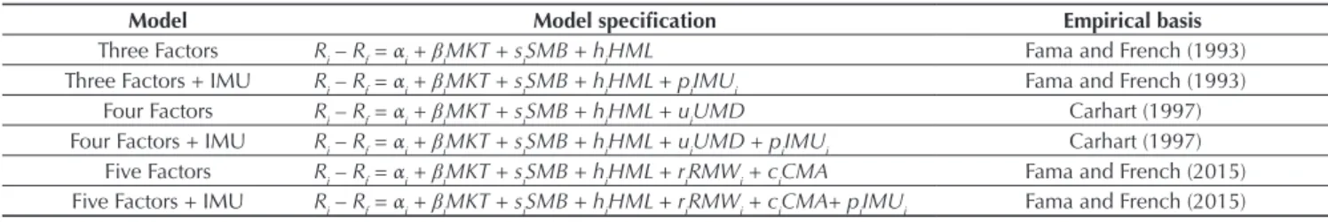
Table 1 displays the speciications of models estimated in this study, which were based on Easley et al. (2005) and Mohanram and Rajgopal (2009).
Table 1 Models tested and their respective empirical bases
Model Model speciication Empirical basis
Three Factors Ri – Rf = αi + βiMKT + siSMB + hiHML Fama and French (1993)
Three Factors + IMU Ri – Rf = αi + βiMKT + siSMB + hiHML + piIMUi Fama and French (1993) Four Factors Ri – Rf = αi + βiMKT + siSMB + hiHML + uiUMD Carhart (1997) Four Factors + IMU Ri – Rf = αi + βiMKT + siSMB + hiHML + uiUMD + piIMUi Carhart (1997)
Five Factors Ri – Rf = αi + βiMKT + siSMB + hiHML + riRMWi + ciCMA Fama and French (2015) Five Factors + IMU Ri – Rf = αi + βiMKT + siSMB + hiHML + riRMWi + ciCMA+ piIMUi Fama and French (2015)
Source: Prepared by the authors.
3.5 Dependent Variables
he dependent variable consists of the average daily excessive return on the stock portfolios in relation to the CDI [Ri – Rf], formed according to the procedure adopted by Fama and French (2015). For creating the portfolios, the main variable ‘size’ was retained and the
Table 3 Portfolios formed having the variables size and VPIN as a basis to create the factor IMU
Portfolio Initials Description
Small and Low SL Intersection between stocks from the group small for the variable size and stocks with low VPIN value Small and High SH Intersection between stocks from the group small for the variable size and stocks with high VPIN value Medium and Low ML Intersection between stocks from the group medium for the variable size and stocks with low VPIN value Medium and High MH Intersection between stocks from the group medium for the variable size and stocks with high VPIN value Big and Low BL Intersection between stocks from the group big for the variable size and stocks with low VPIN value Big and High BH Intersection between stocks from the group big for the variable size and stocks with high VPIN value Source: Prepared by the authors.
���
=
��
+
��
+
��
3
−
��
+
��
+
��
3
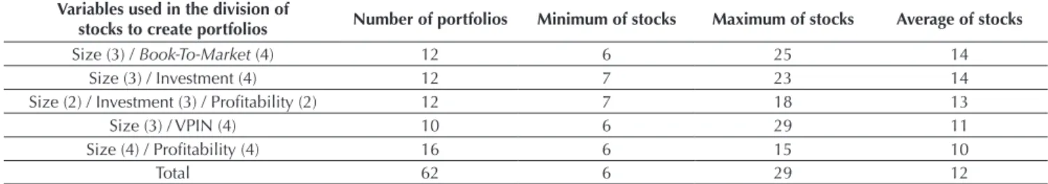
Table 2 Information on portfolios created through the intersection of stocks divided into groups based on the variables: size, book-to-market, investment, proitability, and VPIN
Variables used in the division of
stocks to create portfolios Number of portfolios Minimum of stocks Maximum of stocks Average of stocks
Size (3) / Book-To-Market (4) 12 6 25 14
Size (3) / Investment (4) 12 7 23 14
Size (2) / Investment (3) / Proitability (2) 12 7 18 13
Size (3) / VPIN (4) 10 6 29 11
Size (4) / Proitability (4) 16 6 15 10
Total 62 6 29 12
The column ‘Variables’ indicates which variables are used to build the portfolios. The values in parentheses refer to the breakpoints used in the division of stocks, e.g. (3) indicates that the stocks were divided into 3 groups. The intersections between the stocks were analyzed according to the values of variables, thus the portfolios were formed. Therefore, the number of portfolios consists in the multiplication of breakpoints for each variable. Attention is drawn to the fact that 2 portfolios were excluded from the combination Size and VPIN.
Source: Prepared by the authors.
3.6 Independent Variables
For the creation of a factor related to information risk, irst, the stocks were divided into 3 groups having their
market values as a basis. At the same time, the stocks were divided into 2 groups: low and high VPIN. Finally, we calculated the weighed return on each intersection (Table 3).
hus, the factor IMU was obtained as shown in (6):
he reasons supporting the creation of the IMU lie on the relation between the probability of privileged negotiations and the return on shares. Easley et al. (2002) found a positive correlation between these 2 variables. According to these authors, stocks with higher PIN values have higher required return and, consequently, higher cost of capital. In this study, we observed that the correlation between VPIN and return was 0.0141 with p = 0.0003. Despite the low value, it is possible to have a premium for investment in stocks with greater toxicity of the order lows.
For creating the other factors, the procedures conducted by Fama and French (1993, 2015) and Carhart
(1997) were followed. he factor SMB used in the 3- and 4-factor models proposed by Fama and French (1993, 2015) and Carhart (1997) was calculated by taking return on the intersection of stocks with low market value and low, medium, and high book-to-market and subtracting return on the intersection of stocks with high market value and low, medium, and high book-to-market. he factor HML was created through return on the intersection of stocks with high book-to-market and the groups low and high market value subtracted from return on the intersection of stocks with low book-to-market and low and high market value. he factor moment was obtained by taking return on the intersection of stocks with high
Table 4 Descriptive statistics of the VPIN for the entire sample between 05/01/2014 and 05/31/2016
Number of stocks Minimum Maximum Average Standard deviation
142 0 1 0.4548 0.2218
Source: Prepared by the authors.
past return and low and high market value, subtracted from return on the intersection of stocks with low past return and low and high market value.
For the factor size used in the 5-factor models proposed by Fama and French (2015), we took return on the intersection of stocks with low market value and the other factors, subtracted from return on the intersection of stocks with high market value and the other factors. he factor HML was created through return on the intersection of stocks with high book-to-market and low and high market value subtracted from return on the intersection of stocks with low book-to-market and low and high market value.
For the proitability-related factor (RMW), we took return on the intersection of stocks with high proitability and low and high market value, subtracted from return on the intersection of stocks with low proitability and low and high market value. Finally, for the investment factor (CMA), return on the intersection of stocks with low investment and low and high market value was
subtracted from return on the intersection of stocks with high investment and low and high market value.
3.7 Bootstrap Portfolio Simulation
Bootstrap simulation was used to analyze which combination of factors optimizes the explanation of returns on the portfolios. he application of this method consisted in selecting returns on the portfolios created by resampling with replacement, and the models were estimated under each of them, thus calculating the coeicients of each regression. Ater obtaining the regression intercepts, the Average F-test was applied. he application of this test was needed, because data simulation generates linear dependence between them, making impossible an inversion of the covariance matrix with regression residuals, needed to use the GRS test. For the moments in which no simulated data were used, the GRS test was applied following the steps proposed by Fama and French (1996, 2015).
4. ANALYSIS OF RESULTS
4.1 VPIN Results
he result for VPIN calculation is displayed in Table 4. A comparison of the results provided by Barbedo et al. (2009) and Martins and Paulo (2013, 2014) faces
difficulties inherent to the procedures used in each investigation. Barbedo et al. (2009) and Martins and Paulo (2013, 2014) applied the PIN, in addition to using algorithms to classify the purchase and sale orders. hus, a comparison of studies in other markets using the VPIN.
4.2 VPIN by the BM&FBOVESPA Listing Segment
Regarding the different BM&FBOVESPA listing segments, it was expected that companies in the New
Market (NM) segment, which have, in theory, greater transparency than those in the segments Level 1 (L1), Level 2 (L2), and Traditional (Trad), had lower VPIN. To analyze this hypothesis, daily VPIN was calculated for each segment (Table 5).
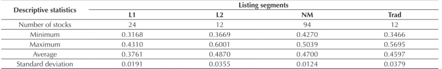
Table 5 Daily VPIN descriptive statistics per BM&FBOVESPA listing segment
Descriptive statistics Listing segments
L1 L2 NM Trad
Number of stocks 24 12 94 12
Minimum 0.3168 0.3669 0.4270 0.3466
Maximum 0.4310 0.6001 0.5039 0.5695
Average 0.3761 0.4870 0.4700 0.4597
Table 6 Descriptive statistics of daily VPIN per group, according to stock market capitalization
Descriptive statistics Groups
Small Medium Large
Minimum 0.5582 0.3544 0.2793
Maximum 0.7134 0.4565 0.3528
Average 0.6364 0.3989 0.3164
Standard deviation 0.0284 0.0164 0.0123
Source: Prepared by the authors.
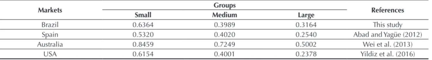
Table 7 Comparison between the VPIN calculated by size groups in different markets
Markets Groups References
Small Medium Large
Brazil 0.6364 0.3989 0.3164 This study
Spain 0.5320 0.4020 0.2540 Abad and Yagüe (2012)
Australia 0.8459 0.7249 0.5002 Wei et al. (2013)
USA 0.6154 0.4001 0.2378 Yildiz et al. (2016)
Source: Prepared by the authors.
We observe that the Level 2 VPIN was the highest among the BM&FBOVESPA listing segments, followed by the New Market, Traditional, and inally Level 1. It is worth noticing that the number of stocks in each segment is very diferent, and New Market is the segment with the largest number of companies. his fact strongly impacts the results by segment, as the analysis by market value explains.
In order to statistically verify the diference between the average VPIN values for the segments, the Student’s
t-test was used. he results point out rejection of the null hypothesis for equal values regarding the average VPIN values for all segments. It was expected that the values presented by the NM would be signiicantly lower than those for the other segments, especially the Traditional. he results found were, however, contrary to expectations. It was found that the segment L1 had the lowest VPIN for the sample analyzed and that the segment L2 had the highest average VPIN within the period concerned.
4.3 VPIN Analysis by Market Value of Stocks
One of the main results of studies that applied the PIN
and, more recently, the VPIN, is that the probability of privileged trading is lower for stocks from big companies. For the VPIN, e.g. the disparity between buying and selling volumes is not so pronounced for larger capitalization irms, thus reducing their low toxicity level. Abad and Yagüe (2012) were the irst to verify this relation in stocks traded in the Spanish market. Wei et al. (2013) and Yildiz, Van Ness and Van Ness (2016) found evidence to support such a claim in studies in the Australian and U.S. markets, respectively. Having this in mind, we sought to verify the relation between the VPIN and companies’ value in the Brazilian stock market.
To investigate this relation, stocks were divided into 3 groups named as small, medium, and large, having about 47 stocks each, related to their average daily market value. he irst clue relating the VPIN to company size came from the correlation between these 2 variables. he result for correlation was -0.3080 and p = 0. Such a value was expected, given the constant empirical evidence of the negative relation between VPIN and size. In order to deepen the analysis of this relation, the descriptive statistics for each group was calculated (Table 6).
Table 6 shows the relation veriied in the studies that applied the VPIN to comparisons between the market capitalization of stocks. here is a signiicant diference between the VPIN for low capitalization stocks in the
In general, the results obtained for medium and large companies in the Spanish and U.S. markets were close to those in the Brazilian market. We may highlight that the VPIN for stocks from the Brazilian companies shows a behavior similar to that of companies in the markets mentioned above, with negative correlation to company size. In general, the VPIN calculated for the domestic market, i.e. 0.4548, is not so diferent from that of the Spanish (0.3960) and U.S. (0.4178) markets.
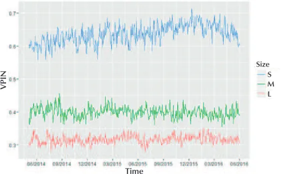
Returning to the analysis of the VPIN characteristics regarding company size, Figure 1 shows the VPIN behavior for each group. We can observe the substantial diference in the toxicity level of stocks concerning their market values. he small group showed a daily VPIN always above 0.55, while the medium group was around 0.40, with slight peaks reaching 0.45. he large group remained more stable, with the lowest standard deviation among the 3, with a maximum of 0.35.
Figure 1 Evolution of daily VPIN for stock size groups.
S: small stocks group; M: medium stocks; L: large stocks in market value.
Source: Prepared by the authors.
Size S M L
VPIN
Time
A substantial diference was found in the VPIN for stocks regarding the variable size, the explanation for VPIN behavior in the BM&FBOVESPA segments may be contained in the market values of stocks constituting each segment. Out of the 47 companies in the small group, 36 are in the New Market segment, which has 94 stocks in total, leading the average NM VPIN to increase substantially. Excluding the small group stocks, the NM VPIN would drop to 0.3418, a igure signiicantly lower than the current VPIN for the segment. For the L1 segment, among its 24 stocks, 1 is within the small
group, 11 within the medium group, and 12 within the large company group, causing the VPIN to be taken down, and this might explain the fact that L1 shows the lowest VPIN among the segments. If the small and medium
Regarding the segment L2, out of the 12 stocks that constitute it, 6 come from the small group, 3 from the
herefore, the hypothesis that company size and its VPIN are negatively correlated was veriied through the sample analyzed in the national stock market. Such evidence is in line with that expected and observed in the international literature.
4.4 Analysis of the 3-, 4- and 5-Factor Models and the Factor Based on the VPIN (IMU)
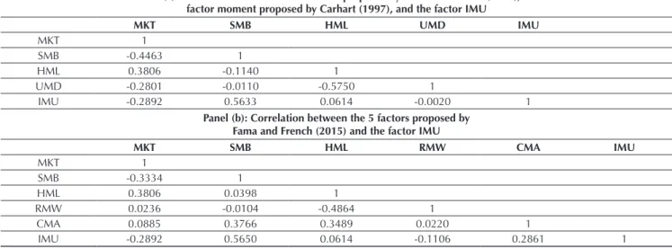
he irst step to analyze the performance of models refers to the correlation between their factors (Table 8). We notice through panel (a), in Table 8, that the IMU showed a moderate and negative correlation to the market factor, which is close to that reported by Easley et al. (2005) and Mohanram and Rajgopal (2009). Regarding the factors HML and UMD, the IMU did not show a signiicant correlation, with p = 0.1643 and 0.9638.
It is noticed that the correlation of greater weight
for the factor constructed by the VPIN is to the SMB. It is possible that return on stocks with higher VPIN are those of small companies, while stocks with lower VPIN represent the larger stocks, and the explanation for a strong correlation between the 2 factors lies on their construction.
When analyzing the correlations between the 5 factors proposed by Fama and French (2015) and the IMU – panel (b), in Table 8 –, it is observed that, even in diferent methodologies, the IMU has a slightly stronger correlation to the factor size. Another moderate and positive correlation arises between the IMU and the CMA. In general, the results do not resemble those presented by Fama and French (2015), except for the positive correlation between the factors CMA and HML. Again, the factors MKT and SMB show a moderate and negative correlation, while for Fama and French (2015) there is a correlation with the same magnitude, but positive.
Table 8 Correlation between the 3, 4 and 5 factors proposed by Fama and French (1993, 2015) and Carhart (1997) and the factor IMU
Panel (a): Correlation between the 3 factors proposed by Fama and French (1993), the factor moment proposed by Carhart (1997), and the factor IMU
MKT SMB HML UMD IMU
MKT 1
SMB -0.4463 1
HML 0.3806 -0.1140 1
UMD -0.2801 -0.0110 -0.5750 1
IMU -0.2892 0.5633 0.0614 -0.0020 1
Panel (b): Correlation between the 5 factors proposed by Fama and French (2015) and the factor IMU
MKT SMB HML RMW CMA IMU
MKT 1
SMB -0.3334 1
HML 0.3806 0.0398 1
RMW 0.0236 -0.0104 -0.4864 1
CMA 0.0885 0.3766 0.3489 0.0220 1
IMU -0.2892 0.5650 0.0614 -0.1106 0.2861 1
Source: Prepared by the authors.
4.4.1 Results of factor model regressions.
In order to present the results regarding the regressions estimated, there is a need to apply econometric tests that aim to test the statistical robustness of the models analyzed. Three tests were performed to verify, respectively, whether there is multicollinearity, whether the regression residues are autocorrelated, and whether the latter are heteroskedastic. he irst test, variance inlation factor (VIF), tests whether the explanatory variables are correlated, something which might afect the estimation of their coeicients. Following Gujarati (2006), VIF values above 10 indicate multicollinearity. It
was veriied that, in none of the 6 models, the result of VIF for the variables was high. herefore, the results indicate there is no multicollinearity between the variables, and it is possible to include them in a regression model with no apparent loss in the coeicient estimates.
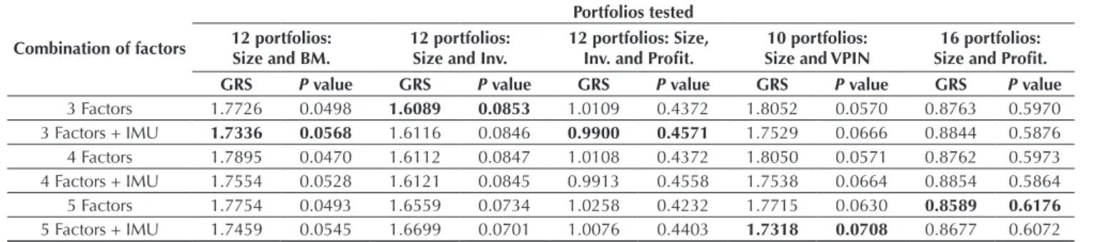
Table 9 GRS test for the 3-, 4-, and 5-factor models plus the factor IMU
Combination of factors
Portfolios tested 12 portfolios:
Size and BM.
12 portfolios: Size and Inv.
12 portfolios: Size, Inv. and Proit.
10 portfolios: Size and VPIN
16 portfolios: Size and Proit. GRS P value GRS P value GRS P value GRS P value GRS P value
3 Factors 1.7726 0.0498 1.6089 0.0853 1.0109 0.4372 1.8052 0.0570 0.8763 0.5970
3 Factors + IMU 1.7336 0.0568 1.6116 0.0846 0.9900 0.4571 1.7529 0.0666 0.8844 0.5876
4 Factors 1.7895 0.0470 1.6112 0.0847 1.0108 0.4372 1.8050 0.0571 0.8762 0.5973
4 Factors + IMU 1.7554 0.0528 1.6121 0.0845 0.9913 0.4558 1.7538 0.0664 0.8854 0.5864
5 Factors 1.7754 0.0493 1.6559 0.0734 1.0258 0.4232 1.7715 0.0630 0.8589 0.6176
5 Factors + IMU 1.7459 0.0545 1.6699 0.0701 1.0076 0.4403 1.7318 0.0708 0.8677 0.6072
Size: Size; BM: Book-to-Market; Inv.: Investment; Proit.: Proitability. The best combination of factors for each portfolio set is highlighted in bold.
Source: Prepared by the authors.
Having these results in mind, it is concluded that the OLS estimators are suicient for a concise estimation of the models’ coeicients.
Table 9 shows the results for the GRS test applied to the portfolio sets. It is veriied that, for the portfolios constructed having size and book-to-market as a basis, adding the factor IMU to the 3-, 4-, and 5-factor models leads to improvement in their performance. For the portfolios constituted by company size and investment, adding the IMU does not entail signiicant diferences in relation to the traditional models. A detail to be highlighted is that the 5-factor model showed worse performance than the 3- and 4-factor models for this set of portfolios.
What can be veriied is that no model has performed better regardless of the set analyzed. Fama and French
(2015) show that the 5-factor model has a signiicant improvement over the 3-factor model for the 7 portfolio sets analyzed by them. In this study, the 5-factor model was better in those sets created through the variables size and VPIN and size and proitability. Portfolio formation based on proitability presented the best explanation level considering the models as a whole. When formed by book-to-market, investment, or VPIN, the models did not perform satisfactorily.
hrough the results presented by the GRS test, there are clues that an information-related factor, when added to the traditional factor models, is adequate to explain returns. In order to analyze this hypothesis more deeply, we regress the factors based on Mohanram and Rajgopal (2009) and Fama and French (2015).
4.4.2 Analysis of the relations between systematic risk factors.
his procedure, performed by Mohanram and Rajgopal (2009) and Fama and French (2015), aims to test whether the regression intercepts are statistically diferent from 0. An intercept equal to 0 would mean that the factor is not priced and that its predictive power is already incorporated to the existing factors.
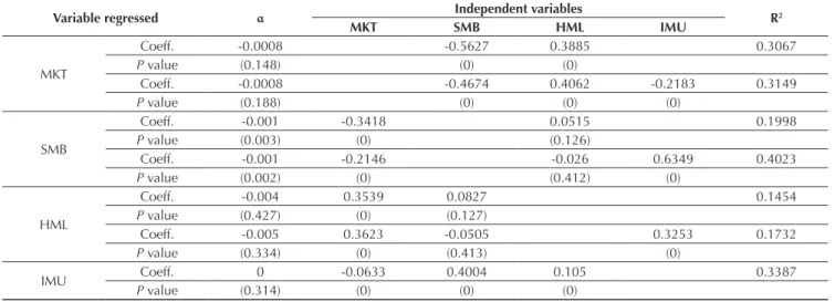
Table 10 shows the estimates for the 3-factor regressions proposed by Fama and French (1993) and the factor IMU. he factor SMB presents an intercept statistically diferent from 0, i.e. the other factors do not incorporate it to returns. When the IMU is added, there is a substantial increase in the regression R2. his is probably due to the
strong positive correlation of 0.56 between the 2 elements. However, despite this increased explanatory power of
regression, the factor SMB is still not captured by the others.
Table 10 Three-factor regression proposed by Fama and French (1993) and the IMU
Variable regressed α Independent variables R2
MKT SMB HML IMU
MKT
Coeff. -0.0008 -0.5627 0.3885 0.3067
P value (0.148) (0) (0)
Coeff. -0.0008 -0.4674 0.4062 -0.2183 0.3149
P value (0.188) (0) (0) (0)
SMB
Coeff. -0.001 -0.3418 0.0515 0.1998
P value (0.003) (0) (0.126)
Coeff. -0.001 -0.2146 -0.026 0.6349 0.4023
P value (0.002) (0) (0.412) (0)
HML
Coeff. -0.004 0.3539 0.0827 0.1454
P value (0.427) (0) (0.127)
Coeff. -0.005 0.3623 -0.0505 0.3253 0.1732
P value (0.334) (0) (0.413) (0)
IMU Coeff. 0 -0.0633 0.4004 0.105 0.3387
P value (0.314) (0) (0) (0)
Coeff.: Coeficient.
Source: Prepared by the authors.
Table 11 Four-factor regression proposed by Carhart (1997) and the IMU
Variable regressed α Independent variables R2
MKT SMB HML UMD IMU
MKT
Coeff. 0 -0.5776 0.2938 -0.2133 0.3183
P value (0.159) (0) (0) (0)
Coeff. 0 -0.4928 0.3177 -0.2108 -0.1913 0.3242
P value (0.195) (0) (0) (0.004) (0.019)
SMB
Coeff. -0.001 -0.35 -0.0181 -0.1906 0.215
P value (0.004) (0) (0.666) (0)
Coeff. -0.001 -0.2227 -0.1033 -0.2002 0.6376 0.4197
P value (0.003) (0) (0.005) (0) (0)
HML
Coeff. -0.0002 0.1976 -0.0201 -0.7281 0.3795
P value (0.556) (0) (0.667) (0)
Coeff. -0.0003 0.2064 -0.1485 -0.7251 -0.3144 0.4059
P value (0.433) (0) (0) (0) (0)
UMD
Coeff. 0 -0.0807 -0.1099 -0.3781 0.3451
P value (0.869) (0) (0) (0)
Coeff. 0 -0.0736 -0.1547 -0.39 0.1119 0.3507
P value (0.950) (0.004) (0) (0) (0.02)
IMU Coeff. 0 -0.0557 0.4111 0.141 0.0933 0.3443
P value (0.320) (0) (0) (0) (0.020)
Coeff.: Coeficient.
Source: Prepared by the authors.
In the analysis of 4-factor regressions proposed by Carhart (1997), depicted in Table 11, it is veriied that the factor UMD had the highest p values for its intercepts,
i.e. 0.869 and 0.95, the latter refers to adding the factor IMU. his means there is strong evidence that the other factors completely capture the factor UMD.
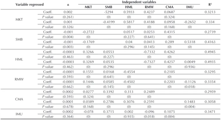
Finally, concerning the two-factor regressions added by Fama and French (2015), depicted in Table 12, the HML is again captured by the other factors. he factors
Table 12 Five-factor regression proposed by Fama and French (2015) and the IMU
Variable regressed α Independent variables R2
MKT SMB HML RMW CMA IMU
MKT
Coeff. 0.002 -5294 0.5933 0.4237 0.0687 0.3213
P value (0.261) (0) (0) (0) (0.324)
Coeff. 0.001 -0.4199 0.5817 0.4188 0.0958 -0.2652 0.334
P value (0.326) (0) (0) (0) (0.168) (0)
SMB
Coeff. -0.001 -0.2722 0.0517 0.0253 0.4315 0.2739
P value (0.004) (0) (0.227) (0.641) (0)
Coeff. -0.001 -0.1769 0.04 0.0413 0.289 0.5318 0.4163
P value (0.003) (0) (0.296) (0.145) (0) (0)
HML
Coeff. -0.0003 0.3266 0.0553 -0.7332 0.4262 0.4945
P value (0.463) (0) (0.227) (0) (0)
Coeff. -0.0003 0.3269 0.0535 -0.7327 0.4257 0.0049 0.4935
P value (0.462) (0) (0.296) (0) (0) (0.936)
RMW
Coeff. -0.0001 0.1551 0.0168 -0.4554 0.2105 0.3295
P value (0.593) (0) (0.641) (0) (0)
Coeff. -0.0001 0.1446 0.0585 -0.4502 0.2203 -0.1126 0.3354
P value (0.662) (0) (0.145) (0) (0) (0.018)
CMA
Coeff. 0.0002 0.0277 0.3392 0.313 0.2489 0.2959
P value (0.593) (0.324) (0) (0) (0)
Coeff. 0.0001 0.0389 0.2786 0.3076 0.2591 0.1483 0.3058
P value (0.678) (0.168) (0) (0) (0) (0.004)
IMU Coeff. 0.0002 -0.078 0.3715 0.002 -0.096 0.1075 0.3471
P value (0.364) (0) (0) (0.935) (0.018) (0.004)
Coeff.: Coeficient.
Source: Prepared by the authors.
herefore, through the regression estimates of factors displayed in tables 10 to 12, it can verify that the 2 main factors responsible for explaining return on the portfolios analyzed seem to be the MKT and the SMB, and the others are incorporated as other factors are added to regressions.
In order to verify which combination of factors results in the best model, the procedure established by Fama and French (2015) is adopted, i.e. analysis of GRS test results for various model arrangements.
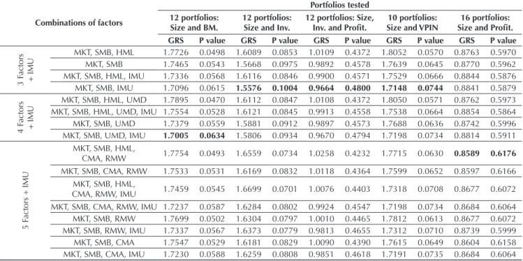
4.4.3 Results for the GRS test in various model combinations.
To find the model that best explains portfolio returns, Fama and French (2015) test various variable
Table 13 GRS test for 3-, 4-, and 5-factor model variations and the factor IMU
Combinations of factors
Portfolios tested 12 portfolios:
Size and BM.
12 portfolios: Size and Inv.
12 portfolios: Size, Inv. and Proit.
10 portfolios: Size and VPIN
16 portfolios: Size and Proit. GRS P value GRS P value GRS P value GRS P value GRS P value
3 F
actors
+ IMU
MKT, SMB, HML 1.7726 0.0498 1.6089 0.0853 1.0109 0.4372 1.8052 0.0570 0.8763 0.5970 MKT, SMB 1.7465 0.0543 1.5668 0.0975 0.9892 0.4578 1.7639 0.0645 0.8770 0.5962 MKT, SMB, HML, IMU 1.7336 0.0568 1.6116 0.0846 0.9900 0.4571 1.7529 0.0666 0.8844 0.5876 MKT, SMB, IMU 1.7096 0.0615 1.5576 0.1004 0.9664 0.4800 1.7148 0.0744 0.8841 0.5879
4 F
actors
+ IMU
MKT, SMB, HML, UMD 1.7895 0.0470 1.6112 0.0847 1.0108 0.4372 1.8050 0.0571 0.8762 0.5973 MKT, SMB, HML, UMD, IMU 1.7554 0.0528 1.6121 0.0845 0.9913 0.4558 1.7538 0.0664 0.8854 0.5864 MKT, SMB, UMD 1.7379 0.0559 1.5881 0.0912 0.9897 0.4573 1.7688 0.0636 0.8742 0.5996 MKT, SMB, UMD, IMU 1.7005 0.0634 1.5806 0.0934 0.9670 0.4794 1.7198 0.0734 0.8814 0.5911
5 F
actors + IMU
MKT, SMB, HML,
CMA, RMW 1.7754 0.0493 1.6559 0.0734 1.0258 0.4232 1.7715 0.0630 0.8589 0.6176 MKT, SMB, CMA, RMW 1.7533 0.0531 1.6169 0.0832 1.0118 0.4364 1.7599 0.0652 0.8597 0.6166
MKT, SMB, HML,
CMA, RMW, IMU 1.7459 0.0545 1.6699 0.0701 1.0076 0.4403 1.7318 0.0708 0.8677 0.6072 MKT, SMB, CMA, RMW, IMU 1.7237 0.0587 1.6284 0.0802 0.9924 0.4547 1.7198 0.0734 0.8684 0.6064 MKT, SMB, RMW 1.7699 0.0502 1.6304 0.0797 1.0010 0.4465 1.7812 0.0613 0.8677 0.6072 MKT, SMB, RMW, IMU 1.7337 0.0567 1.6373 0.0779 0.9813 0.4655 1.7312 0.0710 0.8739 0.5999 MKT, SMB, CMA 1.7547 0.0529 1.6181 0.0829 1.0090 0.4390 1.7615 0.0649 0.8604 0.6158 MKT, SMB, CMA, IMU 1.7230 0.0588 1.6259 0.0808 0.9851 0.4618 1.7191 0.0735 0.8684 0.6064
The column Models shows which factor combinations were used as independent variables in the explanation of portfolio returns (dependent variable in the regressions) evidenced in the other columns.
The best combination of factors for each portfolio set is highlighted in bold. Size: Size; BM.: Book-to-Market; Inv.: Investment; Proit .: Proitability.
Source: Prepared by the authors.
Analyzing the set of portfolios formed by stock size and book-to-market, it is veriied that, among the 16 factor arrangements analyzed, the one showing the best performance consisted in the factors MKT, SMB, UMD, and IMU. An issue arises when including the UMD improves the model performance, considering that it was the one with the lowest intercept and the highest p values in Table 11. he explanation lies on the relation between UMD and HML. Analyzing the UMD regression with the other factors, it is veriied that the HML shows the highest absolute coeicient among the variables, hence indicating that this might be the factor that better captures the UMD return variations. In unreported results, regressions of this factor with the MKT, SMB, and later by adding the IMU, there is a substantial decrease in the p value of the intercept, and this suggests these factors cannot fully capture the factor UMD, leaving margin to play a role in explaining portfolio returns.
It is also veriied that adding the IMU improves the performance of all models analyzed. Again, we should seek an explanation for this evidence, since, through factor regressions, it was found that the IMU was captured by the SMB and the HML. he SMB is the factor with the greatest explanatory power regarding the IMU. As the IMU aims to capture the informational part of stocks
and the relation to company size is a consequence of how the capital market deals with the companies’ information content, it is possible that the IMU is able to explain a part of the portfolio return variations not captured by the factor SMB – the part related to information risk –, and this might explain the improved performance of models that include the factor IMU.
In conclusion, it was found that the best factor combinations were those that excluded the HML and included the IMU. he MKT, SMB, and IMU model showed the best performance for 3 out of the 5 portfolio sets. he MKT, SMB, UMD, and IMU model showed better performance for portfolios formed by size and book-to-market, but it also demonstrated good performance in tests with the other sets, except for the size and proitability combination. For the latter, the best combination consisted in the 5-factor model, followed by the 4-factor model (MKT, SMB, RMW, and CMA). he next section works with portfolio return simulations to check which of these factor combinations best explains returns in the sample analyzed.
4.4.4 Model analysis using the Bootstrap method.
−2�ln�� �
�=1
~ χ2 2n
SMB, UMD, IMU; MKT, SMB, HML, RMW, CMA; MKT, SMB, RMW, CMA. We chose to include the 5-factor models proposed by Fama and French (2015) and its restricted version without the factor HML, in order to verify, through simulations, the efect of HML exclusion on the model performance. To do this, the bootstrap
method was used for simulating portfolio returns. To check the hypothesis that intercepts are not statistically diferent from 0, the Average F-test was used. Finally, in order to determine which of these models showed better overall performance, the Fisher’s method was used to combine the models’ p values, as shown by (7):
Table 14 Result of p value combinations by the Fisher’s method
Combinations of factors
Portfolios tested Size (3) and
BM (4)
Size (3) and Inv. (4)
Size (2), Inv. (3) and Proit. (2)
Size (3) and VPIN (4)
Size (4) and
Proit. (4) General
MKT, SMB, IMU 2.06 × 10⁻⁷ 4.22 × 10⁻⁶ 1.38 × 10⁻⁶ 2.91 × 10⁻⁵ 1.92 × 10⁻⁶ 3.55 × 10⁻²⁴ MKT, SMB, UMD, IMU 2.11 × 10⁻⁷ 5.51 × 10⁻⁶ 1.16 × 10⁻⁶ 3.08 × 10⁻⁵ 2.09 × 10⁻⁶ 4.55 × 10⁻²⁴ MKT, SMB, HML, RMW, CMA 1.87 × 10⁻⁷ 5.54 × 10⁻⁶ 1.13 × 10⁻⁶ 2.81 × 10⁻⁵ 2.82 × 10⁻⁶ 4.06 × 10⁻²⁴ MKT, SMB, RMW, CMA 2.29 × 10⁻⁷ 5.38 × 10⁻⁶ 1.11 × 10⁻⁶ 3.21 × 10⁻⁵ 2.27 × 10⁻⁶ 5.22 × 10⁻²⁴
The best factor combination for each portfolio simulation set is highlighted in bold. Size: Size; BM.: Book-to-Market; Inv .: Investment; Proit.: Proitability.
Source: Prepared by the authors.
where ln Xi is the natural logarithm of each p value. he results for p value combinations are shown in Table 14. For each portfolio set, one model outperformed the others.
hus, p value combinations for the 62 simulations – related to the 62 portfolios of the 5 sets formed.
he model MKT, SMB, and IMU, although showing better results for the sets, as displayed in Table 14, did not support in face of the others when applied to simulated data. he inclusion of the factor moment, resulting in the model MKT, SMB, UMD, and IMU, however, managed to maintain a good performance in portfolio simulations, suggesting that the factor UMD can capture return variations in the general sample.
Finally, due to the evidence displayed in Table 13, that including the factor IMU instead of the factor HML,
generally leads to improved model performance, a ith model’s performance, not reported in Table 14, was analyzed: MKT, SMB, RMW, CMA, and IMU. he result of
p value combinations in the simulations was 7.72 × 10⁻²⁴,
i.e. superior to the performance of the model MKT, SMB, RMW, and CMA, i.e. 5.22 × 10⁻²⁴, which indicates that
adding the factor related to information risk led to the improvement in the restricted model proposed by Fama and French (2015).
5. FINAL REMARKS
his study aimed to: (i) analyze the VPIN or the toxicity level of stocks in the Brazilian market; and (ii) verify, through factor models proposed by Fama and French (1993, 2015) and Carhart (1997), whether a systematic risk factor related to stocks’ information content is priced by the BM&FBOVESPA investors.
An average VPIN value of 0.4548 was found, with a standard deviation of 0.2219 for the Brazilian market. In the analysis related to the stock listing segments, it was veriied that the L1 segment showed lower VPIN, followed by the Traditional, NM, and L2. NM stocks were expected to have lower VPIN values, since the
BM&FBOVESPA segmentation objective is providing the investor with greater transparency, which would imply a lower probability of inside trading. he results suggest that the probability of inside trading in the segments is related to the number of companies and the characteristics of stocks that comprise them, especially their market value. hus, the hypothesis stipulated in this research, that the theoretically more transparent segments of the BM&FBOVESPA might have lower probability of inside trading, could not be conirmed.
he hypothesis that there is a negative correlation between size and the VPIN of stocks was corroborated. he results of this study indicate that there is a correlation of -0.3080 between the market value and the companies’ VPIN. he sample analyzed was divided into 3 groups related to the companies’ market value: small, medium, and large. he average VPIN value for these groups was 0.6364, 0.3989, and 0.3164, respectively, indicating a clear decrease in the VPIN as company size increased.
he last hypothesis, regarding the role of a factor related to the information risk of stocks, was analyzed by constructing the factor IMU. his factor was added to the 3- and 5-factor models proposed by Fama and French (1993, 2015) and the 4-factor models proposed by Carhart (1997) and we used, as dependent variables in regressions, the returns on 62 portfolios constructed having size, book-to-market, proitability, investment, and the stock VPIN values as a basis. For all models, adding the factor IMU increased the predictive power of the SMB in the sample analyzed.
In general, the improved model performance by including the IMU was veriied through the GRS test. In order to further investigate this assertion, regressions between the factors were performed. he results indicate that all factors, except the SMB and the MKT are captured by the others at some point. Fama and French (2015) notice that, in the 5-factor model context, the factor HML becomes redundant. In order to verify which of these factors help explaining portfolio returns, the GRS test was applied to various combinations of factors.
he results indicate that the following models showed better performance: MKT, SMB, and IMU; MKT, SMB, UMD, and IMU; MKT, SMB, HML, CMA, and RMW; and MKT, SMB, CMA, and RMW. In addition to corroborating the result found by Fama and French (2015), that the factor HML is redundant for the 5-factor model, this claim was extended to the 3- and 4-factor models, and it was found that, when present, the HML afects the models’ performance.
In order to extend these conclusions, the bootstrap procedure of portfolio returns was carried out, being regressed through the models mentioned in the previous paragraph. Subsequently, the Average F-test was applied. he results for this test indicate that the model that best explains the simulated returns is MKT, SMB, RMW, and CMA. From the previously presented evidence that the factor IMU helps in the models’ performance, we resorted to return simulations with the model MKT, SMB, RMW, CMA, and IMU. he result found was that the latter had a better performance than the other models, and this provides support for the central hypothesis of this study on information risk pricing in the Brazilian stock market.
hrough the estimate results, it is understood that the factor IMU works as a complement to the factor SMB – the latter is key for the models’ performance – related to the information risk of stocks. he explanation takes place by the way both of them are constructed, since small companies are strongly present in the informed group and the big companies constitute the uninformed group. If these two factors were proxies for each other, the VIF test would have a high value. In addition, it was veriied that the correlation between the 2, although positive, is not enough for one factor to completely incorporate the other, a fact evidenced by the IMU regression with the other factors.
In conclusion, the factor related to information risk seems to play a signiicant role in explaining the return on portfolios created. he market factor and the SMB are the most signiicant in model performance, while the HML is both redundant and harmful. he factors added by Fama and French (2015) help constituting the model that best explains returns on the 62 portfolios analyzed in this study.
REFERENCES
Abad, D., & Rubia, A. (2005). Modelos de estimación de la probabilidad de negociación informada: uma comparación metodológica en el mercado español. Revista de Economia Financeira, 7, 1-37.
Abad D., & Yagüe, J. (2012). From PIN to VPIN: an introduction to order low toxicity. he Spanish Review of Financial Economics,2(10), 74-83.
Agudelo, D., Giraldo, S., & Villaraga, E (2015). Does PIN measure information? Informed trading efects on returns and liquidity in six emerging markets. International Review of Economics and Finance, 39, 149-161.
Aktas, N., Bodt, E., Declerck, F., & Van Oppens, H. (2007). he PIN anomaly around M&A announcements. Journal of Financial Markets, 10, 169-191.
Albanez, T., Lima, G., Lopes, A. & Valle, M. (2010). he relationship of asymmetric information in Brazilian public companies. Review of Business, 31, 3-21.
Albanez, T., & Valle, M. (2009). Impactos da assimetria de informação na estrutura de capital de empresas brasileiras abertas. Revista de Contabilidade e Finanças, 20(51), 6-27. Barbedo, C., Silva, E., & Leal, R. (2009). Probabilidade de
informação privilegiada no mercado de ações, liquidez intra-diária e níveis de governança corporativa. Revista Brasileira de Economia, 63(1), 49-60.
Borochin, P., & Rush, S. (2016). Identifying and pricing adverse selection risk with VPIN (SSRN Working Paper). Retrieved from https://papers.ssrn.com/sol3/papers.cfm?abstract_ id=2599871
Breeden, D. (1979). An intertemporal asset pricing model with stochastic consumption and investment opportunities. Journal of Financial Economic, 7, 265-296.
Brennan, M., Huh, S., & Subrahmanyam, A. (2015). Asymmetric efects of informed trading on the cost of equity capital.
Management Science, 62(9),2460-2480.
Carhart, M. (1997). On persistence in mutual fund performance.
Journal of Finance,52(1), 57-82.
Chiah, M., Chai, D., Zhong, A., & Li, S. (2016). A better model? An empirical investigation of the Fama-French ive-factor model in Australia. International Review of Finance, 16(4), 595-638.
Duarte, J., Hu, E., & Young. L. (2015). What does the PIN model identify as private information? (SSRN Working Paper). Retrieved from https://papers.ssrn.com/sol3/papers. cfm?abstract_id=2564369
Duarte, J., & Young, L. (2009). Why is PIN priced? Journal of Financial Economics, 91, 119-138.
Easley, D., Engle, R., O’Hara, M., & Wu, L. (2008). Time-varying arrival rates of informed and uninformed trades. Journal of Financial Econometrics, 6(2), 171-207.
Easley, D., Hvidkjaer, S., & O’Hara, M. (2002). Is information risk a determinant of asset returns? he Journal of Finance, 52(5), 2185-2221.
Easley, D., Hvidkjaer, S., & O’Hara, M. (2005). Factoring
information into returns. Journal of Financial and Quantitative
Easley, D., Kiefer, N., O’Hara, M., & Paperman, J. (1996). Liquidity, information, and infrequently traded stocks. he Journal of Finance, 51(4), 1405-1436.
Easley, D., López de Prado, M., & O’Hara, M. (2011). he microstructure of the “Flash Crash”: low toxicity, liquidity crashes, and the probability of informed trading. he Journal of Portfolio Management, 37(2), 118-128.
Easley, D., López de Prado, M., & O’Hara, M. (2012). Flow toxicity and liquidity in a high frequency world. Review of Financial Studies, 25, 1457-1493.
Easley, D., López de Prado, M., & O’Hara, M. (2016). Discerning information from trade data. Journal of Financial Economics,
120(2), 269-286.
Easley, D., & O’Hara, M. (1987). Price, trade size, and information in securities markets. Journal of Financial Economics, 19, 69-90.
Fama, E. (1970). Eicient capital markets: a review of theory and empirical work. he Journal of Finance, 25(2), 383-417. Fama, E., & French, K. (1993). Common risk factors in the returns
on stocks and bonds. Journal of Financial Economics, 33, 3-56. Fama, E., & French, K. (1996). Multifactor explanations of asset
pricing anomalies. he Journal of Finance, 51(1), 55-84. Fama, E., & French, K. (2015). A ive-factor asset pricing model.
Journal of Financial Economic, 116, 1-22.
Fama, E., & French, K. (2016a). Dissecting anomalies with a ive-factor model (SSRN Working Paper). Retrieved from https:// papers.ssrn.com/sol3/papers.cfm?abstract_id=2503174 Fama, E., & French, K. (2016b). International tests of a ive-factor
asset pricing model (SSRN Working Paper). Retrieved from https://papers.ssrn.com/sol3/papers.cfm?abstract_id=2622782 Fama, E., & French, K. (2017). Choosing factors (SSRN Working
Paper). Retrieved from https://papers.ssrn.com/sol3/papers. cfm?abstract_id=2668236
Flister, F., Bressan, A., & Amaral, H. (2011). CAPM condicional no mercado brasileiro: um estudo dos efeitos momento, tamanho e book-to-market. Revista Brasileira de Finanças,
9(1), 105-129.
Fortunato, G., Motta, L., & Russo, G. (2010). Custo de capital próprio em mercados emergentes: uma abordagem empírica no Brasil com downside risk. Revista de Administração Mackenzie, 11(1), 92-116.
Gibbons, M., Ross, S., & Shanken, J. (1989). A test of the eiciency of a given portfolio. Econometrica, 57, 1121-1152.
Glosten, L., & Milgrom, P. (1985). Bid, ask and transaction prices in a specialist market with heterogeneously informed traders.
Journal of Financial Economics, 14, 71-100.
Gujarati, D. (2006). Econometria básica. São Paulo: Campus. Hwang, L.-S., Lee, W-J., Lim, S-Y., & Park, K-H. (2013). Does
information risk afect the implied cost of equity capital? An analysis of PIN and adjusted PIN. Journal of Accounting and Economics, 55, 148-167.