analysis from the censuses of 2000 and 2010
Eli Izidro dos Santos
Universidade Estadual de Santa Cruz / Programa em Economia Regional e Políticas Públicas (Perpp) Ilhéus / BA — Brazil
Ícaro Célio Santos de Carvalho
Fundação Getulio Vargas / Escola de Administração de Empresas de São Paulo (FGV EAESP) São Paulo / SP — Brazil
Ricardo Candéa Sá Barreto
Companhia de Água e Esgoto do Ceará (Cagece) / Diretoria Jurídica Fortaleza / CE — Brazil
he article aims to collaborate with the analysis about poverty in the state of Bahia, studying the spatial behavior of poverty in the state in 2000 and 2010, using the Municipal Poverty Index (MPI). he MPI allowed the creation of a ranking of municipalities, which in comparison with the ranking based on the Municipal Human Develop-ment Index (MHDI) in the same years analyzed, was efective for measuring the spatial poverty in the state. he study found evidence of a pattern of spatialization as well as the existence of clusters of regional poverty. It is a multidimensional study using variables such as income, education, housing and health.
Keywords: cluster; spatial distribution; MHDI; poverty.
Pobreza multidimensional no estado da Bahia: uma análise espacial a partir dos censos de 2000 e 2010 Este artigo teve como intuito realizar uma análise do comportamento espacial da pobreza no estado da Bahia nos anos 2000 e 2010, a partir do cálculo do Índice Municipal de Pobreza (IMP), colaborando com as análises da pobreza já realizadas para o estado. O índice permitiu a criação de rankings municipais de pobreza, que em comparação com o ranking do Índice de Desenvolvimento Humano Municipal (IDHM), nos mesmos períodos em análise, mostraram-se eicientes para mensuração da pobreza espacial na região. Com isso, encontraram-se evidências de um padrão de espacialização, bem como a existência de clusters de pobreza regional. Para este estudo foram utilizadas, além da renda, outras variáveis como educação, habitação e saúde, o que caracteriza o trabalho como multidimensional.
Palavras-chave: cluster; distribuição espacial; IDHM; pobreza.
Pobreza multidimensional en el estado de Bahia: un análisis espacial de los censos de 2000 y 2010 Este trabajo tiene como objetivo colaborar con el análisis de comportamiento de la pobreza espacial en el estado de Bahia, en 2000 y 2010 a partir del cálculo del Índice de Pobreza Municipal (PIM), con el in de colaborar con el análisis de la pobreza en el estado. El índice permitió la creación de rankings de pobreza municipales, que en comparación con el ranking del Índice de Desarrollo Humano (IDHM) durante los mismos periodos de revisión fueron efectivas para la medición de la pobreza espacial en la región. Por lo tanto, se encontraron pruebas de un patrón de espacio, así como la existencia de clusters regionales de pobreza. Para este estudio se utilizaron además de los ingresos, otras variables como la educación, la vivienda y la salud, que cuenta con el trabajo como multi-dimensional.
Palabras clave: cluster; distribución espacial; IDHM; pobreza.
DOI: http://dx.doi.org/10.1590/0034-7612152341
Article received on July 21, 2015 and accepted on March 22, 2017.
1. INTRODUCTION
According to data collected by Instituto Brasileiro de Geograia e Estatística (IBGE, 2011), there is a
slight fall on income inequality in the last few years, although there are great diferences in income throughout Brazilian’s territory, especially in big cities. According to 2010 Census, 25% of Brazilian have a per capita income of R$ 188,00 per month, and 50% with a per capita income of R$375,00, which means that 75% of Brazil’s population were living with less than the minimum wage of 2010, which in that year was R$510,00.
According to Lacerda and Neder (2010), the economic growth process in developing countries, especially from 1960, has showed some deformations in the interconnection between income’s increase and poverty’s end. Such deformations refer to the fact that many authors confuse economic growth and development. he process of development occurs when there is an increase in income’s equality improving the life conditions of the poor. If there is only economic growth and no improvement or a decay in the life conditions of the poor, it is not possible to state that a development process has occurred. herefore, poverty cannot be treated and analyzed by the unidimensional look of income. It is necessary to expand the studies on poverty, in order to understand the basic needs of individuals, such as nourishment, health, education, etc. In this sense, there is a new perception over poverty, which is attributed as multidimensional.
Despite the importance gained within specialized literature, especially in economic scene, this theme it is not new, since it has always been present in any hystorical frame. However, with the in-tensiication of debates on economic growth and development in the 1960’s, especially in third-world
countries, the study on poverty received a great level of attention. Yet, according to Superintendência
de Estudos Socioeconômicos da Bahia (SEI, 2008), it is necessary to develop more studies, especially focusing in other dimensions besides income.
Nevertheless, assuming that poverty does not limit itself to income is not enough to obtain good outcomes. If the object of analysis and its behavior are not properly known, any attempts to elaborate and evaluate politics against poverty and, mostly, understanding this reality in a consistent way be-come extremely limited, in order to intervene in a positive and long-lasting way. hus, as a complex phenomena, the study of poverty needs an analysis that involves not only individual’s income, but also other aspects that are related to its event and that are necessary to human’s development such as health conditions, education, habitation, among others.
herefore, in the search for identifying clusters of poverty in the state of Bahia, a municipal po-verty ratio was calculated, with data collected in Demographic Census of 2000 and 2010, for all 417 cities, which analysis was developed using spacial methods. his study has as main goal developing a spacial analysis of poverty in the state of Bahia from 2000 to 2010. Its speciic goals were: (1) me-asuring poverty in the state of Bahia from 2000 to 2010; (2) analyze spacially poverty in Bahia; (3) identify the regions in the state with biggest poverty concentration.
multidi-mensional ratio of poverty, that allows comparisons of the outcomes, revealing some independence between multidimensional poverty and poverty by income.
Besides this introduction, the paper presents a literature review with the main theoretical appro-aches towards this theme, the methodological framework with the main methods used to measure poverty in the state of Bahia, as well as the data sources, the outcomes analysis with the rate of MPI, inal considerations and references used in the conception of this study.
2. LITERATURE REVIEW
Understanding how poverty has behaved throughout the years leads to a comprehension on how its conception has been changing. In this sense, its history shows how the social context needed appro-aches that could better explain poverty. hus, it was possible to understand the need of expanding the studies from an unidimensional look to studies with other variants on this theme.
Some conceptions on poverty were developed since the last century, although there is a complex conceptualization of the term, due to its subjective nature. Besides that, the study may be focused in two ways: the irst one with an economic perspective in which only income is used, and the second one an analysis that incorporates other variants despite the economic ones, such as criminality that deprives citizens. Poor cities may have the same income, basic sanitation, piped water levels, among others. Yet, they may have diferent criminality levels. Violence in some poor cities is much superior to other with the same standard of living.
According to Crespo and Gurovitz (2002), in the last century it was developed three general ideas: (1) survival; (2) basic needs; and (3) relative deprivation. In the irst case, the focus is more restrained
and it has prevailed from the 19th to the 20th century, original from the work of english nutritionists,
it showed that the income of the poor was not enough to maintain the individual’s physical perfor-mance. he second case, it was expanded in the 1970’s, in which other variables were incorporated, such as basic sanitation, piped water, health, education and culture to poverty studies. he third and last case received more attention from the 1980’s on, in which the concept received a more rigid and broader focus, searching for a scientiic formula and comparisons between international studies, especially those who emphasized the social aspect. his idea was strengthened by Amartya Sen, the main theorist of this new conception of poverty.
In this sense, according to Kageyama and Hofmann (2006),the idea of poverty refers to some
To Sen (2000), the characteristic of “absolute poverty” does not mean neither temporal or cultural invariability, neither a focus on nourishment and food, it being a focus to evaluate deprivation in absolute terms instead of more relative criteria.
Relative poverty contrasts to absolute conceptions and proposes the use of a perspective that refers to real deprivation conditions, especially in comparison with other individuals. According to Townsend (1962), “many people have been uneasily aware of the problems of deining necessities like housing, clothing, or fuel and light”. his means that individuals are in poverty situation when they do not have resources for daily activities in the society they belong, being excluded from the socially desirable lifestyle. Related to subjective poverty, according to Martini (2009:10),
[...] here are three present deinitions in the studies. First of all, it can be considered poor the individuals who state they have less resources than what is enough to aford their basic needs. Secondly, this idea can be linked to the principle of basic needs, in a way that poverty is observed by the research, among each family of population, related to whice are their basic needs and comparing it to their real income. Finally, it can be linked to the concept of relative poverty. In this case, being poor is extended to having an individual feeling of owning less than what is necessary to fulill social commitments, in familiar, cultural, social and professional positions terms that each individual presents.
On the other hand, the studies on poverty were recently seen through a diferent look from tho-se applied in the last century. he studies of Amartya Sen (2000) on the dynamic nature of poverty revealed a new horizon of research, in which other variables beyond income were incorporated to poverty analysis, which are described as studies on capabilities deprivation. To Crespo and Gurovitz (2002), “capability” means possible self-realizations. herefore, capability is a kind of freedom: the freedom to be able to achieve self-realization or the freedom to have diferent lifestyles. As an example, a wealth person who decides to adere to fasting by his/her choice, may have the same performance of someone poor who starves. However, the irst person has a “capability set”, diferent from the second. he irst may choose to eat well and be well nourished in an impossible way compared to the second (Crespo and Gurovitz, 2002).
According to Sen (2000), freedom narrows the idea of poverty under the lens of income, expanding and dinamizing new studies. he multidimensional concept of poverty was deined as an old ideia with new arrangements, which characterizes the wideness of the term, in which the economic, social and structural dimensions are involved (Poggi, 2004; Conconi and Ham, 2007). According to IBGE (2011), the discussions on poverty indicators in Brazil still need to be deepened, because they still are very incipient. he federal government, as an example, uses many frames to implement social programs, such as the income distribution policy “Bolsa Famí-lia”, which considers poor the people who have a monthly income of R$ 140,00 or less. However,
there are other indicators such as Pesquisa dos Orçamentos Familiares (POF), which analyzes
consumption, considering it less volatile than income and a representative of the real expenses in food and other goods.
because the choice of the dimensions that will be the object of study and which variants will be used depend on the working goal and on the concept of poverty used by the researcher.
To Lacerda (2009), the main diiculty is to ind a good indicator capable of measuring the multi-mensional nature of poverty. he author highlights that, unlike studies on the unidimulti-mensional light of income, there is not a set of established and solid measures in the multidimensional approach, in the form of a sole ratio that relects all the multidimensional context.
While there is consensus among the researchers of poverty on how imprecise it is, there is no consensus on the nature of this imprecision and on how to capture it. Even among those who use the income poverty line, there is some concern related to how imprecise this measure is; however, such imprecision is attributed to the lack of information available to the researcher rather than to the nature of the studied phenomena.
As shown by Silva and Barros (2006), on the importance of scalar indicators of multidimensio-nal poverty, it is worthy to note that there is not a single way for its contruction. In each step of this process some dilemmas emerge, such as: which are the most relevant dimensions? Which variables and its weights should be adopted? Which method of aggregation of the poverty dimensions should be used? Among other questions.
his fact illustrates the importance of using the Municipal Poverty Index (MPI), that en-compasses income, education, health and habitation. According to Ávila (2013), despite using quantitative data, this ratio focus on individual quality of life, not being restrained to monetary quantiication of poverty. hus, in applied studies, in particular reports of human development,
the main indicator of multidimensional poverty used has been the Índices de Pobreza Humana
(HPI – Human Poverty Index) proposed by Anand and Sen (1997), which inpired MPI. he HPI was incorporated to the Human Development Report of PNUD, from 1997, with the speciic goal to measure poverty, using the same variants of Human Development Index (HDI). Nevertheless, it mainly focuses on the poor and adopts a perspective on individual deprivations. he HPI aims at measuring the size of the deicit in the same dimensions considered by HDI (Ávila, 2013; La-cerda, 2009).
Despite the limitations imposed by such methodology, it shows to be acceptable because it not only measures poverty as it tries to understand it, considering dimensions related to individuals’ quality of life. hus, the understanding of these indices allows the creation of public politicies capable of meeting individual’s needs, and reveal themselves much more eicient than methods that only adopts the income dimension (Ávila, 2013; Lacerda, 2009).
herefore, the next section presents a short description of the steps needed to build a poverty index.
3. METHODOLOGY
3.1 BUILDING A MUNICIPAL POVERTY INDEX FROM THE METHODOLOGY OF HPI
from the methodology of the Human Poverty Index (HPI), created by Sudhir Anand and Amartya Sen (1997). he Exploratory Analysis of Spacial Data and the Global and Local Moran Index also compose this framework, which enable the spacement of poverty and inequality of cities in the state of Bahia under the multidimensional lens.
For the present research, a chart with the indicators of deprivation for each one of the cities of the state was created, in order to allow for the calculations for each index. Later, it was organized the ranking of the cities of Bahia for each calculated index. A comparative analysis of the hierarchies was made, searching the consistency of the indexes, as a way of explaining its use in spacial analysis.
In verifying the consistency of the indexes it was used the ranking of the Índice de Desenvolvimento
Humano Municipal (IDHM — Municipal Human Development Index) of 2000 and 2010, published on Brazil’s Human Development Atlas (PNUD, 2013).
herefore, as already highlighted, the methodology of HPI was initially proposed by Anand and Sen in 1997 and is part of the studies of the United Nations (UN) on human development and poverty ight in the world. According to Ávila (2013), while HDI analyzes average advances in poverty ight, the HPI measures the degree of deprivation of people. Nevertheless, it is important to highlight that, for Anand and Sen (1997), the fact that HPI uses three dimensions to measure deprivations — being one of them composed by three variables, and the other two by only one — may create a problem related to weighting dimensions.
he solution suggested by the authors was to measure the mean of the three variables that compose the economic dimension. According to Anand and Sen (1997), even recognizing the importance that these three components of human poverty have, it is not possible to assume that they equally afect it. hus, to calculate HPI, they propose the use of a weighted average of the three dimensions as a way to highlight the inluence of the dimension with highest value. However, the authors warn that the valuation of such inluence should not be excessive, since it would cause a masking of the weight of the other dimensions.
hen, HPI measures the deprivations relected in three dimensions of human life:
• poorness related to survival (P1) — percentage of people with life expectancy equal or below 40 years old;
• poorness related to knowledge (P2) — percentage of iliterate adults; and
• poorness related to life standards (P3) — composed by three variables: percentage of people with no access to healthcare (P31); percentage of people with no access to drinking water (P32); percentage of children with less than ive years old in a undernourished situation (P33).
hus, deprivation related to life standards is:
P3 = (P31 + P32 + P33) / 3 (1)
And the formula for HPI is:
IPH = [1/3 (P3
It is important to highlight that the indicators used to measure deprivations are percentuals, which makes the calculation of HPI easier, since these indicators are already standardized between 0 and
100, according to Technical Notes of the Human Development Report (PNUD, 2006). An important
assumption is that all three deprivations that compose HPI have the same relative values and that they sum together. he inal value of HPI indicates which proportion of the population is afected by the analyzed deprivations. he higher the percentage, the greater is the deprivation degree (Anand and Sen, 1997).
Ater data collection, it was calculated the Municipal Poverty Index (MPI) from the chosen va-riables, present in chart 1.
CHART 1 DIMENSIONS AND VARIABLES THAT COMPOSE MPI
DIMENSION (D) DEPRIVATION (P)
Habitation and sanitation (HS) 5 or + people in one house (IBGE) No bathroom/toilette (IBGE) No drinking water (IBGE) No garbage collection (IBGE) No sewage treatment (IBGE)
Education (E) No instruction/Sem instrução/basic education incomplete (IBGE)
Health (S) Infant Mortality Index (PNUD; Ipea; FJP)
Income (R) Until 1/4 minimum wage (SM) or no income (IBGE)
Fonte: Adapted from Ávila (2013).
Following the methodological framework, PMI is presented as follows:
Di = 1
(
S
Pij
)
(3)n
In which:
Di = dimension to be calculate;
Pij = deprivation that composes the derived variant;
i = number that indicates the dimension to be calculated (i = 1, ..., 4);
j = number of the deprivation that composes the dimension to be calculated (j = 1. ..., 5); e
n = amount of deprivations that compose the dimension.
Applying the weighted average to dimensions (Di) and rewriting them: HS = D1, E = D2, S = D3,
IMP =
{
1[Da1 + Da2 + Da3 + Da4]
}
1
a (4)
n
Which means: D = Di; i = 1, ..., n
In general formula, there is:
IMP =
[
SDai]
1
a (5)
n
In which:
n = amount of dimensions that compose the index; and
a = weightening factor of the dimensions that compose the index.1
his index can be presented in a more generic way, enabling a separate analysis of each dimension that compose it or even other dimensions or variables which are not study objects of this work. he three indexes used in this study are presented as it follows:
IMP1 =
{
1[HSa + Ea + Sa + Ra4]
}
1
aa
= n = 4 (6)
n
IMP2 =
{
1[HSa + Ea + Sa + Ra4]
}
1
aa
= n = 3 (7)
n
IMP3 =
{
1[Ra]}
1
aa
= n = 1 (8)
n
And inally there is:
Di = 1
(
S
Pij
)
n = 5 para HS, n = 1 para E, S e R (9)n
Since it was proposed to compare spacial distribution of multidimensional poverty in Bahia with poverty only measured through the income lens, it was used three indexes derived from general for-mula. he irst (IMP 1) includes four dimensions previously deined (HS, E, Sd and R); the second (IMP 2) was calculated only with non monetary dimensions (HS, E and Sd); and the third (IMP 3)
was measured only with monetary dimension (R)2.
1 To deine the value of α, it was made a test with α = 3 and α = 4. he diference between the indexes was small, and it was arbitrarily
chosen to use a α = n. Although, there must be extra careful to avoid excessive weight on the more accentuated deprivations, if the number of dimensio is high.
3.2 EXPLORATORY ANALYSIS OF SPATIAL DATA (EASD)
According to Anselin (1988), the Exploratory Analysis of Spatial Data (EaSd) uses georeferenced data and is usually used to test the existence of spacial patterns, such as spacial heterogeneity and spatial dependence, which indicates coincidence in similar values in neighboring regions. his technique considers distribution and data relationship in space. he EaSd is a useful methodology in the study of the processes of spatial propagation because it identiies the patterns of spatial self-correlation, that is, spatial dependence between geographic objects.
hus, for spatial analysis of indexes, it was deined a matrix with two spatial weights (W), that according to Almeida (2008), is the way to express a given spatial arrangment of interactions resulting from the phenomena in study, as a irst step for EaSd. However, considering the existance of spatial self-correlation, it was used the statistics I of Moran Global, which according to Almeida (2012), it is the most accepted way to identify and test it. However, when dealing with a great number of data, there is always the occurrence of spatial dependence. herefore, it was used the statistics I of Moran Local, which enables the identiication of spatial clusters where comparison was not made between cities, but between its local indicators and their neighbors, thus verifying if there are, or there are not, patterns of local concentrations.
To Almeida and partners (2008), the main goal of this method is to describe spatial distribu-tion, the associated spatial patterns, the possible spatial clusters, verify the existence of diferent spatial regimes or other ways of spatial instability (non stationary) and identifying untipical spa-tial observations, the outliers. However, these authors highlight that for implementing EaSd it is necessary to deine a matrix of spatial weights (W). According to Almeida and partners (2008), this matrix is the way to express a determined spatial arrangement of resulting interactions of the phenomena in study. According to these authors, it is likely to suppose that, in the study of several phenomena, neighboring regions have a stronger interaction among themselves than regions that are not contiguous. In a similar way, regions far from one another would have a smal-ler interaction. In this case, in which distance between regions matters in deining the strength of interaction, it would be possible to build a W matrix based on the inverse distance between regions, in order to capture such spatial arrangement of interaction. he authors highlight that
choosing the matrix3 of spatial weights is very important in an EaSd, because the results of the
analysis are sensible to such selection.herefore, considering the idea presented in the contiguous matrix, there is a greater spatial interaction between neighbors than among those who are more distant. Ávila (2013) states that the outcome of this interaction is that poverty indexes inluence and are inluenced by poverty indexes of neighbor cities, and that this inluence decreases ac-cording to the distance.
hus, aiming at spatial self-correlation, Almeida (2012) highlights that the best way to identify and test is through statistics I of Moran, which presents values that range from -1 to 1 as a way of associating the dataset in analysis, which is quite helpful in studying the entire region. However, when
3 he queen and the tower are the main matrixes used. hus, it is considered neighbors of the analyzed unity the areas that are at an
dealing with a great number of areas, it is common that diferent regimes in spatial crowding occur, emerging locals in which spatial depence is evident (Almeida, 2012; Anselin, 1988).
herefore, the matrix and the level of contiguity were initially deined, to later proceed to the analysis itself, through the creation of maps. hus, the spatial self-correlation test was applied of the I of Moran, which indicated that the use of the Queen in the irst order would be more suitable, since it presented a higher level of contiguity, closer to 1, for both periods and indexes, being n accordance with the methodological elements stated by Anselin (1988) and Almeida (2012).
he weight matrix is determined in an exogenous way. It can be deined using contiguity, distan-ce or more complex speciications. Acconding to LeSage (1999), the matridistan-ces of contiguity can be: linear, rook, bishop, double linear, double rook and queen. he queen weights matrix 1 was chosen by EaSdfor presenting a greater value in Moran’s Index when compared to other matrices. he queen
weights matrix 1 considers the regions that share sides and apexes with the region of interest.4
By calculating Municipal Poverty Index (MPI) it was comparatively analyzed the ranking of the cities. It was attempted to verify the consistency of calculated indexes as a way to explain its use in spatial analysis. To verify the consistency of indexes, as already mentioned, it was used the Municipal
Human Development Index (IDHM in portuguese) of 2000 and 2010, published on Brazil’s Human
Development Atlas (PNUD, 2013).
his is an index ranging from 0 to 100; therefore, the inal value of IMP indicates the proportion of poors in the city. his way, higher values mean greater degree of poverty. In this sense, the cities who obtained an index below 20% are considered low in poverty, those who obtained an index from 20% to 49,99% were considered intermediate in poverty, and those with an index beyond 49,99% were considered high in poverty (Ávila, 2013).
3.2.1 GLOBAL INDEX OF MORAN
Global Index of Moran (I) consists on a spatial self-correlation measure that shows the existence or non-existence of spatial groupments for a given variable, that is, the presence of poverty indexes with similar values among neighbors, according to an indicator of interest. his indicator, according to Almeida (2004) is convenient when it is desired a synthesis of spatial distribution of data, as proposed, being an alternative measure of segregation.
According to Almeida and partners (2008), this index enables to verify whether data are spa-tially correlated or not, indicating the level of linear association between vectors observed in time
t (Zt) and the weighted average of neighbor values, or the spatial lags (WZT). When the values of I
are bigger than the expected value, represented by the formula I >E(I) = – 1/n – 1, there is a positive
self-correlation; on the other hand the formula I < E(I) = – 1/n – 1, there is a negative self-correlation.
he positive self-correlation demonstrates similarities between the variables of the studied charac-teristic and its spatial location. When the self-correlation is negative, there is heterogeneity between the variables of the studied characteristic and its spatial location (Almeida, 2004). hus, Moran Index I is expressed in (10):
It= (n/ S0)(zt Wzt/zt zt)t = 1, ..., n (10)
in which: zt represents the vector of n observations for the year t in the condition of deviation related
to average; W is the matrix of spatial weight, whose elements in the main diagonal Wii are equal to 0,
while the elements Wij point the way how region i presents itself spatially connected to region j; and
S0 is th sum of all elements in the matrix of spatil weigh W.
In the present work it is proposed to use statistics I of Moran calculating the matrix of spatial weights normalized in the line, which means, when the sum of elements in each line equals 1, the expression (11), can be written as follows:
It = (zt Wzt/zt zt)t = 1, ..., n (11)
hus, according to Almeida (2004), when the I of Moran results in a value < 0, there is a positive self-correlation (clustering), revealing similarity between the data of the studied characteristic. If the value of 1 is > 0 there will be a negative self-correlation (spatial outlier) stating the dissimilarity between the values of the studied attribute and its spatial location. Finally, if the value of I of Moran equals zero (0), there is no self-correltion among the data.
Nevertheless, the index I of moran is a global measure. In this sense, Almeida (2004) emphasizes that it is not possible to trust only in the global statistics, because they can hide or mask the local patterns of linear spatial association. In this case, the best way out is to use the Local Index of Moran, a measure that enables a complete evaluation of the studied region, enabling an observation of local patterns linearly signiicant to the study.
3.2.2 LOCAL INDEX OF MORAN
Local Index of Moran (ii) enables the identiication of spatial clusters in the way exposed previously to the global index, with the diference of comparing local indicators and its neighbors instead of cities, verifying if there are patterns of local concentration or not. his is possible because the Moran Index presents a value for each region, enabling the identiication of spatial patterns and creating clusters that would represent them.
herefore, the Local Indicator of Spatial Association (Lisa) executes the dissolution of the global indicator of self-correlation in the local contribution of each observation in four categories, each one individually corresponding to a quadrant in the dispersion diagram of Moran. his way, Lisa is calculated through the Local Index of Moran, expressed as follows:
Ii =
(yi – y) S
jwij (yj – y) (12)
S
i (yi – y)
2 / n
Where: wij is the value of the neighbor matrix for the region i with region j in function of distance
Using the hypothesis of randomness, the expected value for local statistics I of Moran is given
by E(Ii) = – wi / (n – 1), in which wi is the sum of the line elements. In this context, the dispersion
diagram of Moran is one of the ways to interpret the statistics I of Moran. According to Almeida and partners (2008), throughout the representation of regression coeicient, there is the possibility to
check the linear correlation between z and Wz in the graph that considers both variables. Highlighting
the speciic case of statistics I of Moran, there is the graph of Wz and z. herefore, the coeicient I of
Moran is given by the declination of the regression curve of Wz against z, which will present its degree
of adjustment. In this sense, the graph of dispersion of Moran is divided in four quadrants, which correspond to four patterns of local spatial association among regions and its respective neighbors.
he irst quadrant exhibits regions with low values for the variable of interest, surrounded by nei-ghbors who present high values, classiied as Low-High (BA in portuguese). In the second quadrant are the regions who present greater values for the variable of analysis, surrounded by regions that equally present high values for the same variable, and it is classiied as High-High (AA in portuguese). he third quadrant is named Low-Low (BB in portuguese), as it is formed by regions whose values of the variable of analysis are low and surrounded by regions in the same situation. he fourth quadrant is High-Low (AB in portuguese), composed by regions with high values for the variable of interest, which present themselves surrounded by regions of low values. In this sense, it is positively spatially self-correlated, that is, clusters of similar values to the regions located in AA (second) and BB (third) quadrants are created. On the other hand, the regions located in BA (irst) and AB (second) quadrants have some negative spatial self-correlation, creating clusters with dissimilar values.
3.3 DATA SOURCE
In the present study, the regions used were cities from the state of Bahia. In this context, the unities are the amount of houses and number of inhabitants of each city to compose the analyzed dimensions. To habitation/sanitation and income dimensions, the unit of analysis is the residence. Regarding health and education dimensions, the unit of analysis is the individual.
It was used in this study data from the Census of 2000 and 2010, for each of the 417 cities in Bahia, obtained in the Sidra Bank of IBGE, available in: <www.sidra.ibge.gov.br/cd/cd2010Serie.asp?o=2&i=P>,
as well as IDHM and Infant Mortality Index, whose data were obtained from Brazil’s Human
Develeo-pment Atlas, created by the Development Program of the United Nations (PNUD, 2013).
It is highlighted the period of 2000 in which only 415 cities were used, since Barrocas and Luiz Eduardo Magalhães did not exist as oicial cities by then.
4. RESULTS AND DISCUSSIONS
his section aims to present and discuss the main results of this study, obtained through the calcu-lation of indexes and the Exploratory Analysis of Spatial Data.
4.1 RANKINGS OF CITIES OF BAHIA RELATED TO POVERTY AND DEVELOPMENT
In this sense, the city that presented the worst poverty situation was Buritirama, when evaluating IMP1, achieving the ratio of 63,93% and Pedro Alexandre for IMP2, with 63,71% in 2000. In 2010, the worst ratio achieved was on Mirante for IMP1, with 65,61% and the city of Caetanos with 66,99% for IMP2. Related to IMP3 the worst result obtained was in Buritirama in 2000 with IMP3 of 63,52% and in 2010 the worst result obtained was in Sitio do Mato, with 58,51%. However, related to IDHM the worst results were obtained in Monte Santo with 0,283 in 2000, and in Itapicuru with 0,486 in 2010. his data suggests that there was a great improvement on the levels of human development in a decade. Similar results were obtained by Lacerda (2009) and SEI (2008).
hese results show the consistency of Municipal Poverty Indexes used in this study, simulta-neously pointing that they can be used to study poverty in the state of Bahia, as well as its spatial distribution. It is clear that the similarity is bigger among cities with the 10 worst results, for every index, both in 2000 and 2010. Moreover, that the less developed cities are the ones with greater poverty indexes.
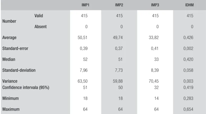
Regarding the descriptive analysis, it can be stated that more than half of the cities of Bahia have multidimensional poverty higher than the average of the state in 2000 (table 1), because it has a median greater than the average, both for IMP1 an IMP2. Analyzing IMP3, it is clear that there is a completely opposing situation, in which the average is greater than the median, showing that less than half of the cities in Bahia are poor.
TABLE 1 DESCRIPTIVE STATISTICS OF POVERTY AND DEVELOPMENT INDEXES IN BAHIA (2000)
IMP1 IMP2 IMP3 IDHM
Number
Valid 415 415 415 415
Absent 0 0 0 0
Average 50,51 49,74 33,82 0,426
Standard-error 0,39 0,37 0,41 0,002
Median 52 51 33 0,420
Standard-deviation 7,96 7,73 8,39 0,058 Variance
Conidence intervala (95%)
63,50 51
59,88 50
70,45 32
0,003 0,419
Minimum 18 18 14 0,283
Maximum 64 64 64 0,654
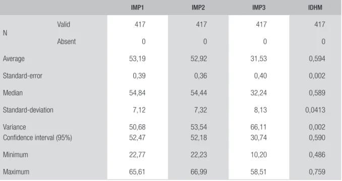
he same can be veriied in 2010, shown in table 2. It is clear, however, an increase of 2,68% in the average of multidimensional poverty of 2010 in relation to 2000. However, the IMP3 has decreased in 2,29%.
TABLE 2 DESCRIPTIVE STATISTICS OF POVERTY AND DEVELOPMENT INDEXES IN BAHIA (2010)
IMP1 IMP2 IMP3 IDHM
N
Valid 417 417 417 417
Absent 0 0 0 0
Average 53,19 52,92 31,53 0,594
Standard-error 0,39 0,36 0,40 0,002
Median 54,84 54,44 32,24 0,589
Standard-deviation 7,12 7,32 8,13 0,0413
Variance
Confidence interval (95%)
50,68 52,47
53,54 52,18
66,11 30,74
0,002 0,590
Minimum 22,77 22,23 10,20 0,486
Maximum 65,61 66,99 58,51 0,759
Source: Elaborated by the authors from the data of Sidra (2011) and Brazil’s Human Development Atlas (PNUD, 2013).
hese data reinforce what research institutes had already announced, a decrease in poverty. Howe-ver, they demonstrate that income is not enough to study poverty and social inequality in Bahia and, in addition to conirming the statements of rankings, they also legitimate the use of indexes to study poverty in the state. According to Moura Jr. and partners (2014), in order for the strategies of poverty reduction to be eicient, they must advance towards acknowledging the speciic needs of individuals inserted in a given social and cultural context, enabling the inclusion of new elements for a broader understanding of the poverty phenomena.
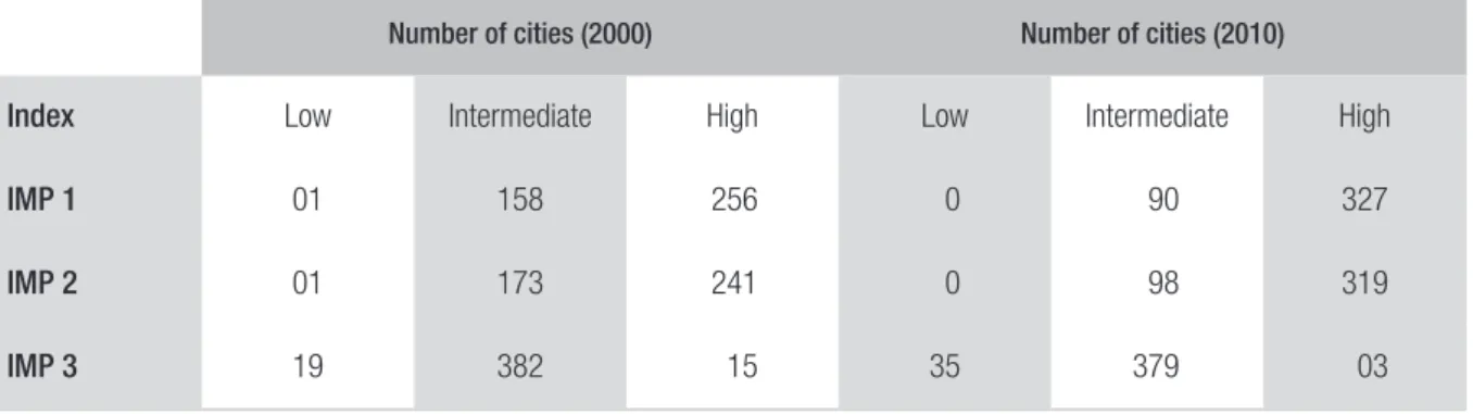
TABLE 3 NUMBER OF CITIES OF BAHIA BY DEGREE OF POVERTY (2000 E 2010)
Number of cities (2000) Number of cities (2010)
Index Low Intermediate High Low Intermediate High
IMP 1 01 158 256 0 90 327
IMP 2 01 173 241 0 98 319
IMP 3 19 382 15 35 379 03
Source: Elaborated by the authors.
Regarding 2010 (chart 3), it can be veriied a similar structure of results when compared to the previous period. his conirms even more the consistency of the indexes used, as well as the results of previous analyses. However, it is clear the increase in multidimensional poverty in the state. Neverthe-less, when comparing only income, there is a signiicant decrease in the high and intermediate poverty intervals, and consequently, an increase on the level of poverty from 19 to 35 cities in this condition. hese results amplify even more the disparity between multidimensional and unidimensional indexes.
4.2 SPATIAL ANALYSIS OF POVERTY IN THE STATE OF BAHIA
he following analysis enables a better look on how poverty, measured by the indexes here calculated, is distributed across Bahia, enabling it to proceed to a higher number of comparisons between poverty through the multidimensional lens and that based on income, unidimensional.
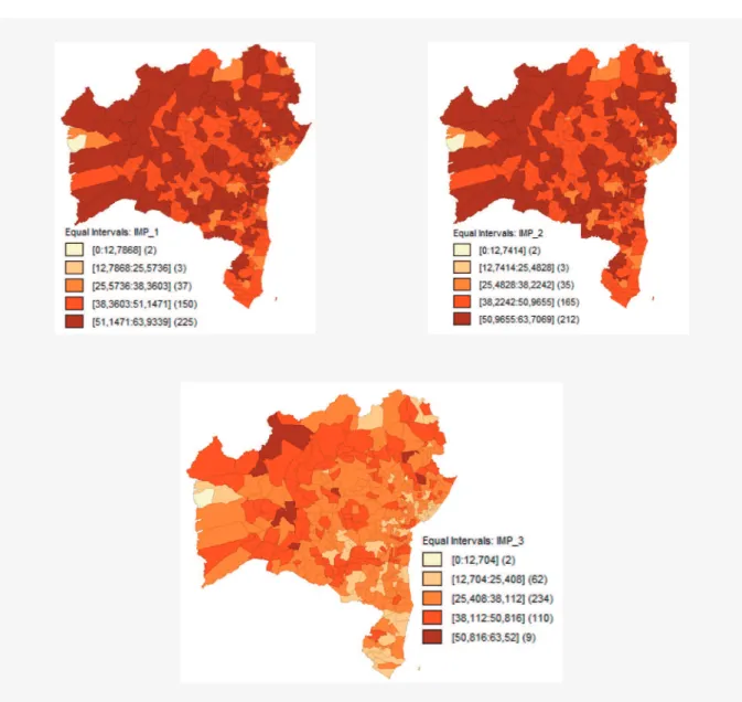
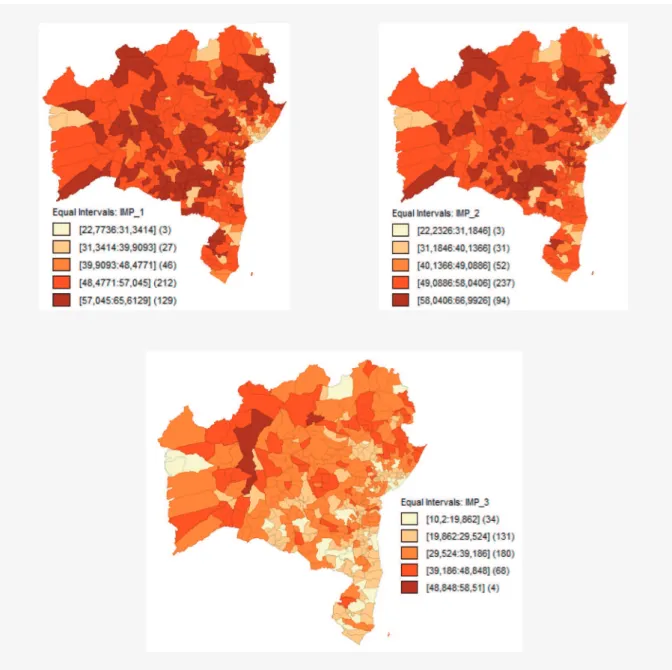
In this sense, the poverty distribution maps in the state of Bahia in 2000 (igure 1) demonstrate the existence of poor and not poor regions, where IMP1 and IMP2 have very similar results, and IMP3, who focuses on income, demonstrates a quite diferent format. he maps conirm what the rankings had already stated, but it difers since it shows the spatialization of poverty.
It can be veriied the presence of clusters of poor and not poor cities, where the number of in-tervals in maps of multidimensional indexes are closer. It is highlighted that the GeoDa 9 sotware uses the maximum and minimum values of each ranking to determine the intervals of analysis, and is diferent from the ones used in the graduation rankings which range from 0 to 100. However, in
the unidimensional poverty map there are 62 cities.5 his demonstrates a big disparity between this
dimension and the multidimensional one. When observing the worst indexes, considering the 4th and
the 5th intervals, disparity gets more clear. he IMP3 presents only 119 cities, while IMP1 and IMP2
register 375 and 377 cities, respectively.
5 he irst chart, the clearest was not considered, since it refers to Barrocas and Luís Eduardo Magalhães which in 2000 were not oicial
FIGURE 1 POVERTY DISTRIBUTION MAPS IN THE STATE OF BAHIA (2000)
Source: Elaborated by the authors.
In 2010 (igure 2), the spatial distribution maps demonstrate how discrepancies between the multidimensional and unidimensional poverty indexes have increased even more in relation to 2000.
Observing the multidimensional maps, the equality on the intervals of cities with better poverty conditions is clear, in order that only three are registered. However, the unidimensional index is more expressive on the interval of cities with better poverty ratio, with 34 cities, pointing a substantial improvement on the unidimensional poverty indexes in relation to 2000.
analyzing the unidimensional map, there are 72 cities in this category, representing an even more accentuated decrease, around 39% in the same period.
FIGURE 2 SPATIAL MAPS OF POVERTY IN THE STATE OF BAHIA (2010)
Source: Elaborated by the authors.
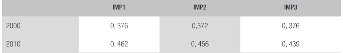
Considering the existence of spatial self-correlation, where the dispersion graph shows the existence or inexistence of spatial groupments, for a determined variable, the statistics I of Moran enables the author to verify if data is or is not spatially correlated, at the same time that it shows the intensity of this relation. In this sense, table 4 exhibits the outomes of each index calculated in this study.
TABLE 4 MORAN INDEX OF IMP1, IMP2 AND IMP3 TO THE STATE OF BAHIA (2000 AND 2010)
IMP1 IMP2 IMP3
2000 0, 376 0,372 0, 376
2010 0, 462 0, 456 0, 439
Source: Elaborated by the authors.
Generally, the indexes displayed have values closer to zero, pointing to a low spatial self-correlation for both periods, with more accentuated values in 2010. At the same time, there is an evidence of an increase on the spatial association degree in the dataset from one decade to another.
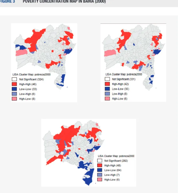
he results already presented indicate the presence of poverty clusters, in both periods of ana-lisys for all indexes. However, the use of local index of Moran enables the identiication of clusters (poverty spots) from the products in the irst index; in this case, it is compared the indicator with their neighbors, verifying if there are local spatial concentrations or not. It is emphasized that it was considered a conidence interval of 99% with 99 disturbances in this study.
It should be highlighted the legend of the colors used in the maps: white means no statistical signiicance; dark red represents high poverty indexes surrounded by cities highly poor; dark blue represents cities with the lowest poverty index surrounded by cities with the same characteristic; light blue shows clusters of low poverty surrounded by cities of high poverty levels; and light red shows clusters of high poverty surrounded by cities of low poverty indexes.
FIGURE 3 POVERTY CONCENTRATION MAP IN BAHIA (2000)
Source: Elaborated by the authors
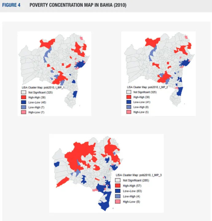
FIGURE 4 POVERTY CONCENTRATION MAP IN BAHIA (2010)
Source: Elaborated by the authors
In relation to IMP3, the analysis reveal that the cities with high poverty indexes surrounded by those of high poverty indexes have increased from 49 to 60, concentrated on the north and northe-astern regions of the state.
In the cities with low poverty index surrounded by cities of low poverty, there was a decrease of 10% in the number of cities in this condition. However, this does not mean that there was an increase of income poverty, but rather, a smaller interaction of cities in this category.
It is clear in this index the presence of bigger High-High clusters, especially on the outback of Bahia, and Low-Low clusters in the metropolitan and Southern region of the state, equal in both periods analyzed, with a slightly displacement of the outback cluster, which was already pointed by previous research, such as Lacerda (2009) and SEI (2008).
hese data reinforce previous analyses that used the global index, at the same time it conirms the statement that poverty studies that take into account only the income variable are not enough to explain the reality of populations who sufer from deprivations in the state of Bahia, suggesting the need for many other multidimensional variables in the studies.
5. FINAL CONSIDERATIONS
Literature on social inequality, poverty and wealth has advanced a lot in the past years, especially regarding its determinants. It can be noticed that these themes have reached some expression in po-litics, and also caught the public’s attention, contributing to an intensiication of the studies that aim to understand the multidimensionality of the phenomena, searching for indicators strong enough to reproduce in an authentic way this problem, and so, to apply helping measures.
When considering the multidimensional nature of poverty, it is needed an indicator that corres-ponds to the multidimensional approach. herefore, this study proposed to calculate an indicator of poverty that its its multidimensional nature, whose methodological basis is similar to that used in HPI. It was also used the analysis os spatial data (Aede), which aimed at understanding the spatializa-tion of poverty in the state of Bahia. herefore, it was used data available in IBGE, through 2000 and 2010 Census, which where compared to IDMH of both periods, available in PNUD (2013), through
Brazil’s Human Development Atlas.
Regarding the spatial analysis, the outcomes conirmed the initial hypothesis of the study, rein-forcing the existence of poverty concentrations in the state of Bahia, no matter the index used in its analysis. It was conirmed in the study that the number of concentration is higher when income analysis is used than when the multidimensional indexes is used, showing a spatial dependence. However, in the multidimensional maps, the clusters are more numerous and more difuse throughout the state, indicating that poverty in this focus is more spatially distributed.
he analyses through this exploratory technique of spatial data evidenced that throughout the years there was an increase of positive self-correlation of poverty in the cities of Bahia, identifying greater High-High and Low-Low clusters in 2010. Another possible change to be observed is that, through the income lens, the majority of poverty clusters have presented a High-High set, indica-ting that the cities that presented a high index of monetary poverty sufered an inluence from their neighbors in the same situation.
It is clear that Bahia must advance in creating and implementing public policies of development and poverty reduction, in a way to estimulate economic growth, especially those capable of generating jobs and income, as well as encouraging an improvement on poor people’s life conditions, such as infrastructure of basic sanitation, better habitation, health and education. As long as these activities become more competitive, through policies developed by local agents, the efect of income generation will enable a greater local/regional development and, therefore, reduce poverty and social inequality. Even understanding that income should not be the only poverty indicator, it is possible to state that it remains as an important element to ight it.
REFERENCES
ALMEIDA, Eduardo. Análise espacial da produtivi-dade do setor agrícola brasileiro: 1991-2003. Nova Economia, v. 17, n. 1, p. 65-91, 2008.
ALMEIDA, Eduardo. Curso de econometria espacial aplicada. Piracicaba: Esalq-USP, 2004.
ALMEIDA, Eduardo. Econometria espacial aplicada. Campinas: Alínea, 2012.
ALMEIDA, Eduardo S.; PEROBELLI, Fernando S.; FERREIRA, Pedro G. Existe convergência espacial da produtividade agrícola no Brasil? Revista de Economia e Sociologia Rural, v. 46, n. 1, p. 31-52, 2008. Available at: <www.scielo.br/scielo.php?script=sci_arttext&pi-d=S0103-20032008000100002&lng=en&nrm=iso>. Accessed on: 13 Jan. 2017.
ANAND, Sudhir; SEN, Amartya. Concepts of human development and poverty: a multidimensional pers-pective. In: Poverty and human development: human development papers. New York: PNUD, 1997. p. 1-19. Available at: <http://clasarchive.berkeley.edu/ Academics/courses/center/fall2007/sehnbruch/ UNDP%20Anand%20and%20Sen%20Concepts%20 of%20HD%201997.pdf>. Accessed on: 5 Feb. 2017. ANSELIN, Luc. Spatial econometrics: methods and models. Boston: Kluwert Academic, 1988.
ÁVILA, José F. Pobreza no Rio Grande do Sul: uma análise exploratória da sua distribuição espacial a partir de indicadores multi e unidimensionais. Dis-sertação (mestrado em economia do desenvolvimen-to) — Faculdade de Administração, Contabilidade e Economia, Pontifícia Universidade Católica do Rio Grande do Sul, Porto Alegre, 2013.
BAHIA. Evolução e caracterização das manchas de pobreza na Bahia (1991-2000). Salvador: SEI, 2008. SILVA, Mirela de C. P. da; BARROS, Ricardo P. Po-breza multidimensional no Brasil. In: ENCONTRO NACIONAL DE ECONOMIA, 2006, Salvador. Anais da Anpec. 2006. p. 1-20.
BRASIL. Indicadores sociais municipais: uma análise dos resultados do universo do Censo Demográfico 2010. Rio de Janeiro: IBGE, 2011.
CONCONI, Adriana; HAM, Andrés. Pobreza multi-dimensional relativa: una aplicación a la Argentina. La Plata: Cedlas, 2007.
CRESPO, Antônio; GUROVITZ, Elaine. A pobreza como um fenômeno multidimensional. Revista RAE. RAE-eletrônica, v. 1, n. 2, p. 1-12, 2002. Available at: <www.scielo.br/pdf/raeel/v1n2/v1n2a03>. Accessed on: 15 Feb. 2017.
FERES, Juan C.; VILLATORO, Pablo. A viabilidade de se erradicar a pobreza: uma análise conceitual e metodológica. Cadernos de Estudos — Desen-volvimento Social em Debate, n. 15. Brasília, DF: Ministério do Desenvolvimento Social e Combate à Fome; Secretaria de Avaliação e Gestão da Infor-mação, 2013.
IBGE. Instituto Brasileiro de Geograia e Estatística.
Indicadores sociais municipais: uma análise dos re-sultados do universo do Censo Demográfico 2010.
Rio de Janeiro: IBGE, 2011.
KAGEYAMA, Ângela; HOFFMANN, Rodolfo. Po-breza no Brasil: uma perspectiva multidimensional.
Economia e Sociedade, Campinas, v. 15, n. 1 (26), p. 79-112, Jan./June 2006.
LACERDA, Fernanda C. A pobreza na Bahia sobre o prisma multidimensional: uma análise baseada na abordagem das necessidades básicas e na aborda-gem das capacitações. Dissertação (mestrado em economia) — Universidade Federal de Uberlândia, Uberlândia, 2009.
LACERDA, Fernanda C.; NEDER, Henrique D. Pobreza multidimensional na Bahia: uma análise fundamentada no indicador multidimensional de pobreza. Revista Desenbahia, v. 7, n. 13, p. 33-70, 2010.
LESAGE, James P. he theory and practice of spatial econometrics. Ohio: University of Toledo, 1999. MARTINI, Ricardo A. Um ensaio sobre os aspectos teóricos e metodológicos da economia da pobreza. Belo Horizonte: UFMG/Cedeplar, 2009.
MOURA JR., James. F. et al. Concepções de pobre-za: um convite à discussão psicossocial. Temas em Psicologia, v. 22, n. 2, p. 341-352, 2014.
PNUD. Programa das Nações Unidas para o Desen-volvimento. Relatório do desenvolvimento humano: a água para lá da escassez: poder, pobreza e a crise mundial da água. New York: PNUD/ONU, 2006. Available at: <www.br.undp.org/content/brazil/ pt/home/library/relatorios-de-desenvolvimen- to-humano/relatorio-do-desenvolvimento-huma-no-20006/>. Accessed on: 12 Feb. 2017.
POGGI, Ambra. Social exclusion in Spain: measu-rement theory and application. Tese (doutorado) — Universitat Autònoma de Barcelona, Barcelona, 2004.
SEI. Superintendência de Estudos Socioeconômicos da Bahia. Evolução e caracterização das manchas de pobreza na Bahia (1991-2000). Salvador: SEI, 2008.
SEN, Amartya. Desenvolvimento como liberdade.
Tradução de Laura Teixeira Mota. São Paulo: Com-panhia das Letras, 2000.
SIDRA. Sistema IBGE de Recuperação Automática.
Censo Demográico 2000. Brasília: Instituto Brasileiro de Geograia e Estatística, Brasília, 2001. Available at: <https://sidra.ibge.gov.br/pesquisa/censo-demo-graico/demograico-2000/inicial>. Accessed on: 10 Jan. 2017.
TOWNSEND, Peter. he meaning of poverty. he Bri-tish Journal of Sociology, v. 13, n. 3, p. 210-227, 1962. VINHAIS, Henrique; SOUZA, André. Pobreza relati-va ou absoluta? A linha híbrida de pobreza no Brasil.
In: ENCONTRO NACIONAL DE ECONOMIA, 2006, Salvador. Anais... Salvador: Anpec, 2006. p. 1-18.
Eli Izidro dos Santos
Master degree in regional economics and public policies from State University of Santa Cruz (PERPP/UESC). E-mail: [email protected].
Ícaro Célio Santos de Carvalho
PhD candidate at Getulio Vargas Foundation, Business Administration School of São Paulo (FGV EAESP). E-mail: [email protected].
Ricardo Candéa Sá Barreto