Rev. Adm. (São Paulo) vol.49 número2

(1)

ISSN 0080-2107

Análise do risco sistemático multi-escalar no mercado inanceiro do Brasil

Neste trabalho, é analisado se a relação entre risco e retorno pre-vista pelo Capital Asset Pricing Model (CAPM) é válida no mercado brasileiro de ações, com base na decomposição discreta de ondale-tas em diferentes escalas de tempo. Essa técnica permite analisar a relação em diferentes horizontes de tempo, desde o curto prazo (2 a 4 dias) até o longo prazo (64 a 128 dias). Os resultados apon-tam que entre os anos de 2004 e 2007 há uma relação negativa ou nula entre risco sistemático e retorno para o Brasil. Como o retorno excedente médio da carteira de mercado em relação ao ativo livre de risco no período foi positivo, seria esperado que essa relação fosse positiva, ou seja, que um maior risco sistemático resultasse em um maior retorno excedente, o que não ocorreu. Portanto, não se observou nesse período uma remuneração adequada pelo risco sistemático no mercado brasileiro. As escalas que apresentaram

a relação risco e retorno mais signiicativas foram as três primei -ras, correspondendo a horizontes de mais curto prazo. Em outras

palavras, ao se tratar diferentemente ano a ano e, em consequência, separar prêmios positivos e negativos, encontra-se em alguns anos

alguma relevância na relação risco retorno prevista pelo CAPM, mas que não persiste ao longo de todos os anos. Portanto, não há

evidência suicientemente forte de que o apreçamento dos ativos

segue o modelo.

Palavras-chave: apreçamento de ações, relação risco e retorno, CAPM, ondaletas, mercado acionário brasileiro.

Analysis of multi-scale systemic risk in Brazil’s

inancial market

Adriana Bruscato Bortoluzzo

Insper Instituto de Ensino e Pesquisa – São Paulo/SP, Brasil

Andrea Maria Accioly Fonseca Minardi

Bruno Caio Fernando Passos

Recebido em 10/agosto/2012 Aprovado em 14/junho/2013

Sistema de Avaliação: Double Blind Review

Editor Cientíico: Nicolau Reinhard

DOI: 10.5700/rausp1143

R

ESU

MO

Adriana Bruscato Bortoluzzo, Mestre e Doutora em Estatística pela Universidade de São Paulo, é Professora Assistente do Insper Instituto de Ensino e Pesquisa (CEP 04546-042 – São Paulo/SP, Brasil). E-mail: adrianab@insper.edu.br

Endereço:

Insper Instituto de Ensino e Pesquisa Rua Quatá, 300

Vila Olímpia

04546-042 – São Paulo – SP

Andrea Maria Accioly Fonseca Minardi, Mestre e Doutora em Administração de Empresas pela Fundação Getulio Vargas de São Paulo, é Professora do Insper Instituto de Ensino e Pesquisa (CEP 04546-042 – São Paulo/SP, Brasil).

E-mail: minardi@insper.edu.br

(2)

1. INTRODUCTION

One of the most often used models in modern inance is

the Capital Asset Pricing Model (CAPM) developed by Sharpe (1964) and Lintner (1965). The model predicts the relation between the risk and the expected return on an asset accord-ing to theexpectations equilibrium regarding the returns on risky assets. The CAPM predicts that the investor only prices the systemic risk, which is measured by the share’s beta, and the investor demands a risk premium equal to the beta multiplied by the market portfolio risk premium. The share’s

beta corresponds to the regression coeficient for excess asset

returns and excess market portfolio returns.

The risk-return relation predicted by the CAPM is widely used to estimate the rate of return demanded to adequately reward the risk that the shareholder assumes. It serves as a benchmark for the minimum required rate of return for implementing a project and is used to determine the fair value of assets. This relation is based on a theoretical market portfolio that is unob-served. In general, market indexes are used as proxies for the theoretical portfolio to estimate the share’s betas.

Ross (1976) proposes the Asset Pricing Model (APT) as an alternative approach for asset pricing. This theory uses various factors to explain asset returns.

Fama and French (1992) analyze the cross-section relation-ship between betas and average returns, allocating the shares in portfolios according to the size of the company and the book to market ratio (the ratio of the book value of equity to its market value). The expected relationship between risk and returns is not observed; that is, it is true that the higher the beta value, the higher the portfolio return average. The authors conclude that there are other systemic risks that are not portrayed in the market portfolio and that size and book-to-market ratio are proxies for these risks.

According to Roll and Ross (1995) the exact relation between

the average return and beta must be satisied if the market index

that serves as a proxy for the theoretical market portfolio is in

the eficient part of the eficient frontier. Whenever we test the CAPM, we are actually testing the eficiency of the market

index rather than the validity of the CAPM.

Studies such as Lakonishok and Shapiro (1984), Mankiw and Shapiro (1986), Breeden, Gibbons and Litzenberger (1989),

and Cochrane (1996) did not ind a signiicant relationship

between systemic risk and return, as would be expected based on the CAPM. Therefore it is questionable if the CAPM is valid in Brazil.

Assuming that the CAPM is valid in Brazil, an issue often pointed in the literature is what procedures result in better betas (see for instance Blume [1971], Cohen, Hawawini, Maier,

Schwartz & Whitcomb (1983), Cecco [1988], Gregory-Allen, Impson & Karaiath [1994]). Should we use higher length of data to produce more stable betas? What frequency (i.e.

daily, weekly, monthly, etc) of time series is best indicated for

calculating betas? Does the aggregation in portfolios improve beta’s stability?

This work analyzes whether the predicted relation between risk and returns based on the CAPM when IBOVESPA is used, is valid in the Brazilian stock market. If market portfolio excess return is positive, we expect that the higher the beta, the higher the asset excess return. If it is negative, we expect that the higher the beta, the lower the asset excess return. This analy-sis is based on discrete wavelet decomposition at different time scales, which permits the use of different time horizons ranging from short-term (2 to 4 days) to long-term (64 to 128 days). Checking different scales horizon allows us to verify what fre-quency allows us to estimate better betas.

The study of the scalar relationship between systemic risk and returns in the Brazilian market offers the investor a more

eficient way of pricing assets and measuring the cost of capital

in a company, facilitating the analysis of investments accord-ing to national standards.

It has been observed that the short-term time scales gen-erate betas that best explain the relationship between risk and returns. Therefore, using more frequent data (as for instance daily data instead of monthly data) is better to estimate betas in Brazil. However, during the period from 2004 to 2007, although the market premium was positive, a negative relation-ship between risk and returns was observed. That is, there was no evidence that Brazilian stocks were priced according to the relationship between risk and return predicted by the CAPM when using IBOVESPA.

This article is organized as follows. Section 2 contains a

literature review; Section 3 presents the theoretical foundations

of the CAPM, discusses its validity and contains a brief review of wavelets, followed by the methodology for estimating sys-temic asset risk using multi-scale decomposition; Section 4 presents the database; Section 5 contains the tables and results of the analysis and a comparison of the results with those of the international literature; and Section 6 presents the study conclusions and a brief summary of what was accomplished.

2. LITERATURE REVIEW

The use of wavelets in inance is recent in the Brazilian

literature. Lima, Kimura, Assaf Neto and Perera (2010) use wavelets to decompose a time series, in conjunction with econo-metric and neural network models, to forecast the data for a 60 kg sack of soy. The results obtained were satisfactory when

using a wavelet ilter in a recurrent neural network. Morettin,

Toloi, Chiann and Miranda (2010) introduce a copula estima-tor based on wavelet smoothing of empirical copulas for time series data and they study the correlation between daily returns of Ibovespa (Brazil) and IPC (Mexico), SP500 and DJIA, and

CAC40 and DAX35. Pimentel and Silva (2011) analyze the correlation among inancial indexes for the Brazilian, American

(3)

investment contribution to the energy of a time-series with wavelet decomposition. The use of wavelets to estimate the systematic risk in the Brazilian market, decomposing the beta on several time scales that represent the short to long term is not yet published in Brazil.

Ramsey and Zhang (1995) and Ramsey and Lampart (1998) used discrete wavelet decomposition to test models in which betas and/or risk premiums varied as time went by. Wavelets are functions with speciic properties used to decompose a time

series over time and in terms of frequency, allowing researchers to work with different time horizons. This, in turn, allows the study of correlations between markets using these time hori-zons. Thus, an analysis of the beta of an asset becomes more robust because the multi-scale decomposition of a series of returns on these assets allows one to observe the risk-return ratio according to the time scale and as from different points of view.

In this way, one can analyze which scale obtains betas that better explain the relationship between risk and returns and

whether a more signiicant return is explained by a higher risk.

Gençay, Whitcher and Selçuk (2003) use wavelets to

decompose a given time series on a multi-scale base to estimate the betas of assets. They use the methodology proposed for the stock markets of the United States, Germany, and the

United Kingdom with the goal of inding the best time scale

for measuring systemic risk.

Gençay et al. (2003) analyze the American economy using daily data from all of the stocks listed in the S&P 500 index

from January 1973 until November 2000 and forming a data

-base with 7,263 observations (28 years). The S&P 500 index

is a proxy for the market portfolio, and the 10-year Treasury Bill is a proxy for the risk-free asset. The results indicate a positive relationship between beta and returns for all time scales, although this relationship is not linear (it forms a smile

shape). The authors observe that the slope and the coeficient of

determination (R2_{) of the regression models grow as the scale} increases (from high to low frequency). They conclude that the relationship between risk and return is multi-scale phenomenon and that the predictions associated with the CAPM are more relevant for an investor with medium to long-term horizons.

In the study of the stock market in Germany, a database was

constructed from all stocks contained in the Xetra DAX (DAX30)

index from January 2000 to December 2001 (except for three, for which, absent values were shown). This process yielded 499 observations. Gençay et al. (2003) consider the DAX30 as market returns and the daily Euro Interbank Offered Rate (EURIBOR) as the risk-free rate. They observe that the third scale (which considers a period from 8-16 days, a medium-term interval) best approximates the estimated average market pre-mium, when compared to the actual one. The estimated market premium in Germany based on the best scale in the period is

-18.5% (3rd level), and the actual premium in the period was

-16% per year. The average excess market return is negative, and the assets with the highest beta have the lowest returns,

resulting in a negative slope for asset returns and beta. These results are in accordance with those predicted by the risk-re-turn ratio; during moments when the market is declining, the

higher the systemic risk, the lower the return.

The database for the United Kingdom includes a random sample of thirty stocks listed in the Financial Time Stock Index (FTSE100) from January 2000 to December 2001 (491 observa-tions). The proxy for the market portfolio is the FTSE100, and the proxy for the risk-free rate is the UK Treasury Bill middle rate with a one-month length of time. The relationship between risk and return is captured with great precision at the highest decomposition levels: that is, in the medium and long term. However, the observed relationship between risk and return is negative, and the actual market premium was -15.6% per year. Thus, the results are in accordance with those predicted by the CAPM risk-return ratio.

Fernandez (2006) analyzes the stock market in Chile using a sample of twenty-four stocks with liquidity of at least 85% that were traded in the Santiago stock exchange from January 1997 to September 2002. As a proxy for the market portfolio, Fernandez uses the Price Index of Selected Stocks (IPSA), whereas the proxy for risk-free assets is the return rates paid on bank deposits within 30 days. The average actual market

premium during the period is -9.06% per year. Although the

coeficients in the model are not signiicant at the 5% signiicance

level, indicating that there is no relationship between risk and returns according to the CAPM, the author conclude that the CAPM model makes better predictions in scale 2 (4 to 8 days) because the estimated market risk premium for this scale (-11.5% per year) is the closest to the actual risk premium.

Rhaeim, Ammou and Mabrouk (2007) study twenty-six highly liquid stocks in the French stock market from January 2002 to December 2005 (1,044 observations, or 4 years). The CAC40 index is used as the market portfolio and the daily EURIBOR as the risk-free rate. The authors conclude that the predictions of the CAPM are more relevant in the short term than in the long term, which makes the French market differ-ent from those of the United States, Germany, and the United Kingdom. The relationship between risk and returns is negative for all the scales and linear only for scales 1, 2, and 6.

Aktan, Mabrouk, Ozturk and Rhaiem (2009) use a database composed of 98 stocks chosen randomly from those listed on the Istanbul Stock Exchange (ISE) during the period from January

2003 to October 2007. Their proxy for the market portfolio is the

ISE-National100 index, and their proxy for risk-free asset returns

is the returns paid daily on bank deposits. They ind a positive relationship between risk and returns that is most signiicant at the 3rd level (8 to 16 days), concluding that the effect of market

returns on an asset is stronger in this time horizon. In addition, the inclination rises according to the increase in the scale (from short to long-term), indicating that the CAPM is more relevant in long-term time horizons than other scales and that the

(4)

Samaei (2012) analyzes the multi-scale systematic risk in Iran, using 15 selected stocks, listed on Tehran Stock Exchange (TSE) Actively traded over June 2004 and June 2009 (1,211 observations). He uses the annual interest rate of the investment bonds issued by the central bank as proxy for the risk-free asset returns and the total price index of the Tehran Stock Exchange (TEPIX) as proxy for the return of market portfolio. The relationship between the return of a stock and its beta is more

robust at medium and short scales (2 to 32 days), indicating that the market is more eficient at irst to fourth scales.

Consistent with works by Fernandez (2006), Rhaeim et al. (2007), Aktan et al. (2009), and Samaei (2012) this article uses the methodology proposed by Gençay et al. (2003), which uses wavelets as a tool for estimating the systemic risk of an asset considering the market portfolio as the systemic risk factor. Toward this end, we analyze the risk ratio for returns on assets Toward this end, we analyze the risk ratiofor returns on assets listed in the São Paulo Stock Exchange (Bovespa) during the period from 2004 to 2007 at different levels. Our

aim is to determine the scale that best relects the beta of an

asset in the Brazilian stock market.

3. METHODOLOGY

3.1. Capital Assets Pricing Model (CAPM)

The Capital Assets Pricing Model (CAPM, proposed by Sharpe [1964] and Lintner [1965]) emerges from the problem maximization for an agent in an environment of uncertainty. According to Blanchard and Fischer (1989), an agent with a horizon of T periods maximizes the function

[1]

where E represents the conditional expectation of the utility function for consumption (U(c_t)) during time t = 0 and where θ is the discount rate over time.

We assume that at time t, an agent chooses to allocate his wealth between a given risk asset n with a stochastic rate of return (liquid) of r_it(i=1,2,…,n) and a risk-free asset with a rate of return r₀_t. The result of the maximization implies n+1

irst-order conditions:

, i=1,2,...,n, [2]

[3]

The agent should choose to consume in such a manner that his marginal utility is equal to the discounted marginal utility for the next period. This condition should be main-tained independently of the asset, whether it is free from risk or not. For assets with risk, the marginal utility during

t depends on the expected value of the product of the mar-ginal utility during t +1 and its rate of return [2]. When the rate of return of the risk-free asset is known during time t, the rate can be determined based on the conditional

expec-tation, resulting in equation [3].

Equations [2] and [3] result in a set of restrictions on

returns on assets and the process of consumption. Thus, these equations provide the equilibrium condition for their returns given the process of consumption. Substituting [2]

with [3], we obtain

[4]

We can also simplify this notation, substituting E[∙|t] for E[∙]

[5]

[6]

Thus, the expected return on asset i satisies the equation

[7]

The higher the covariance of the return on an asset with marginal utility of consumption, the higher the expected return of the equilibrium asset will be. Given that, in equilibrium, the asset provides a hedge for consumption, the agents will be willing to obtain a lower return when the marginal utility of consumption decreases. On the other hand, agents will demand a higher rate of return when the marginal utility of consump-tion increases.

Taking an asset m that is negatively correlated with U'(c_t₊₁), for any risky asset (for example, U'(c_t₊₁) = –γr_mfor any positive γ),

[8]

However, for the asset m, equation [7] implies that

[9]

Substituting [8] and [9] with [7], we obtain

[10]

By deinition, βi is known as the coeficient of regression

(via ordinary least squares) for excess asset returns and excess

market portfolio returns or those of the index. This coeficient

may be obtained using the following equation:

(5)

It may also be derived using an ordinary least squares (OLS) estimator for the following equation:

, [12]

where ε_it is a random shock (white noise).

Thus, we obtain the relationship between systemic risk and the premium via the amount of market risk given by

. [13]

The Brazilian literature in general does not validate the CAPM relation in Brazil, and many papers suggest a mul-tifactor approach. Oliveira and Carrete (2005) and Flister,

Bressan and Amaral (2011) ind that book to market is a rel -evant factor in explaining return. Minardi (2004) and Mussa,

Trovão, Santos and Famá (2007) ind evidence of momen -tum in Brazilian stocks. Lucena and Pinto (2008) observe that size and book-to-market are significant factors in Brazil. Machado and Medeiros (2011) verify that the inclusion of factors such as size, book-to-market, moment and liquidity to the market portfolio improve the predictive power of risk and expected return in Brazil.

3.2. Wavelets

Wavelets are non-sinusoidal functions with limited duration

and a mean equal to zero. They are used to simultaneously decompose time series in terms of time and scale. Unlike Fourier analysis, multi-scale decomposition divides the time-frequency plane into a set of components of high and low frequency. Thus, while Fourier analysis characterizes the global behavior of a time series, wavelets characterize the local behavior of the series.

First, one should consider the formation of an L2₍_ℜ₎

space for all integrable functions of the squared model; that is, based on the dilations and translations of the order (j,k), respectively, of a function ψ(∙). The wave -lets ψ_j,k(t) are formed from the function ψ(t), also called the mother wavelet, using transformations and dilations and form-ing a orthogonal base for . These are given by

. [14]

Each base function depends on two parameters, one of scale (j) and another found in (k). To obtain a representation, the binary dilations 2j_{and dyadic translations k2}-j of ψ(_t_{) should} be considered.

The basic properties that characterize a wavelet are

. [15]

Thus, the function should decrease rapidly towards zero

when |t|→∞. If condition [15] is valid, for any ℜ, 0<ϵ<1, there is an interval of a inite length [–T,T] such that

. [16]

Therefore, the function should be practically null outside the interval [–T,T] for ℜ close to zero. The function ψ(∙) also has the following properties:

, [17]

where ψ^ (w) is a Fourier transformation of ψ (t).

The irst M-1 moments of p(.) are null; that is,

for some [18]

Property [17] is known as the admissibility condition and guarantees that the function of interest f (∙) can be reconstructed from the wavelets transformation. The value of M is related to the degree of smoothness of the wavelet where the greater the value of M, the more regular ψ(∙). Some wavelets have com -pact support, a desirable property related to the fact that the wavelets are located in time. However, not all wavelets generate orthogonal systems. The advantage of working with orthogonal bases is that it allows a perfect reconstruction of the original

signal based on the coeficients of the transformed wavelets. Based on the irst speciication presented regarding the for -mation of a L2₍_ℜ) space, functions ψ

j,k(∙) form an orthogonal

base generated by ψ(∙); then,

[19]

in which

[20]

are the coeficients of the wavelets.

The scalar function ϕ(∙), known as the father wavelet, is the

solution to the equation

[21]

The high-frequency detailed components are captured by the mother wavelets, whereas the low-frequency smooth com-ponents are captured by the father wavelet.

An orthonormal family in L2₍_ℜ_{) is formed via the dilations}

and translations of ℜ(∙); that is,

(6)

The wavelets ψ(∙) may be obtained from the father wave -let as follows:

[23]

in which h_k=(-1)k_l

k-1 and lk and lk are coeficients of the high and low pass ilters, respectively, given by

[24]

[25]

As in this study, a number of applications that facilitate the analysis of wavelets use discrete wavelet transformation

(DWT) to calculate the coeficients near a discrete signal.

For more information on wavelets, see Chui (1992), Ogden

(1997), Morettin (1999) and Percival and Walden (2000).

3.3. Multi-scale variance and covariance

Gençay et al. (2003) introduce the method of systemic risk estimation that uses wavelets to decompose a time series, transforming them to produce multi-scale

coeffi-cients. As indicated in Section 3.1, the estimation of the

asset beta is obtained via equation [11] for each of the (j) levels of the wavelet.

Assuming that the market return structure r_m is stationary,

it is possible to deine multi-scale variance independent of

time, simply called “wavelet variance”, for the market return m associated with level j, such that

[26]

in which c_mjare wavelet coeficients given by [20]. The wave -let variance at level j is the variance of the wavelet coefi -cients of level j.

Taking r_mt and r_it as market returns and the returns on a given asset i, respectively, and applying wavelet

transfor-mation, the vectors of the wavelet coeficients c_mj and c_ij are obtained via decomposition. The wavelet covariance of r_mt and r_it at level j is given by Cov(c_mj,c_ij). Note that the

cova-riance and vacova-riance may be signiicantly different at certain

levels, resulting in different betas for each scale.

Thus, the estimator for the systemic risk of an asset at scale is given by

[27]

4. DATA AND METHODOLOGY

We collect in Bloomberg daily data of Brazilian stocks traded

in BOVESPA from January 5th_{2004 till January 17}th_2007.

Because of the need for a number of observations, to the power of two, a condition imposed by the use of discrete wave decomposition, the missing data were completed with quotes from the following period, including some from the

consecu-tive year. We included in the sample only assets with more than

60% liquidity per year, and the missing data for these assets

were estimated using the Kalman ilter to avoid the large-scale

loss of information due to missing values for the selected assets.

We need a balanced panel, and eliminated stocks that did not have shares traded in all years. Our inal sample has 256 obser -vations for each year.

We used the accumulated Selic and the daily Bovespa indexes (IBOV) as proxies for the risk-free rate and the mar-ket portfolio respectively. The sample contains 1000 trading days: that is, approximately 4 years.

The asset returns were calculated such that r_i,t=Ln(P_i,t⁄ P_{i,t -}₁) where r_i,t and P_i,t represent the quote return of the asset closing price i on date t and the closing price, respectively.

The betas of the assets were estimated according to

for-mula [11] of Section 3.1, where β^

n,j represents the

estima-tor of systemic risk for asset n on scale j, Cov(c_mj,c_cnj) is the

covariance between the wavelet coeficients of excess market

returns (c_mj) and asset n(c_nj) and the jth_{level of} decomposi-tion, and Var(c_mj) is the variance in the wavelet coeficients of the risk premium index of the market at scale j.

The return series were decomposed in 6 levels via the discrete wavelet transformation method using wavelet D(8) such that the first scale is associated with an interval of 2-4 days, the second an interval of 4-8 days, the third an

interval of 8-16 days, the fourth an interval of 16-32 days, the fifth an interval of 32-64 days, and the sixth an inter -val of 64-128 days.

Based on the method proposed by Reinganum (1981), 10 portfolios were formed for each year, all with the same number of equally weighted assets. The assets were ordered according to the estimated betas and placed in the 10

portfo-lios from the largest to the smallest beta. Thus, the irst port -folio is formed from the assets with the lowest betas and the

tenth portfolio from the assets with the highest betas. We then

calculated the average representative beta of each portfolio. After calculating the portfolios for the years from 2004 up to 2007, we created a portfolio with the returns and the betas

averages during the period under analysis.

5. RESULTS

(7)

Table 1 presents the results estimated using ordinary least squares (OLS) regression for the period analyzed as per equa-tion [28]. For demonstraequa-tion purposes, the constants and slopes were multiplied by 100.

, [28]

where r_c-r₀corresponds to excess portfolio returns c; δ_j is the constant for the regression at level j of the wavelet, which, according to CAPM should be zero; λ_j is the slope of the regres-sion at level j of the wavelet, which corresponds to the risk premium of the market portfolio estimated at scale j; β_cj is the beta of portfolio c estimated by OLS at level j of the wavelet; and ν_cj is the random error.

The better the relationship between risk and returns, the

more coeficient λ should approach the historic premium of the

market portfolio. This coeficient corresponds to the slope of

the graphs presented in Figure 1. If the historic market premium is positive, then a positive relationship should be expected

between the excess portfolio returns and the betas. If the historic market premium is negative, a negative relationship should be expected. It is also interesting to observe the constant δ_j. According to CAPM, this constant should be zero.

According to Pettengill, Sundaram, and Mathur (1995), although the investor always demands an ex ante positive premium to invest, based on the ex post returns on assets, these premiums or excess returns may be negative. A pos-itive λ_j (the slope of the regression described in equation [28]) should be expected whenever the excess returns or pre-mium observed ex post is positive, and it should be negative if the observed premium is negative. Therefore, the authors advise that one study the difference between the impact of observed positive premiums and that of negative premiums. Based on these authors’ suggestion, the average year-by-year risk-return ratio was analyzed in different scales.

Detailed graphs and tables for the portfolios for all years and the average for the period can be found in the Appendix, along with the results of the regressions for each level of wave-let decomposition.

Based on the analysis of the results in Table 1, there is a

larger coeficient of determination (R2) from the irst to the third scale, and the estimated risk premiums at lower levels

(with higher frequency) have greater statistical signiicance.

However, one can observe that the constants of the

regres-sions for various scales were signiicant and that the slopes were signiicant in the three irst scales but negative overall,

even though the average historic premium in IBOVESPA is 0.289% per day. That is, the assets and portfolios that possess the greatest systemic risk were not those with the largest posi-tive premiums in the actual market, and the expected relation-ship between risk and returns was not observed.

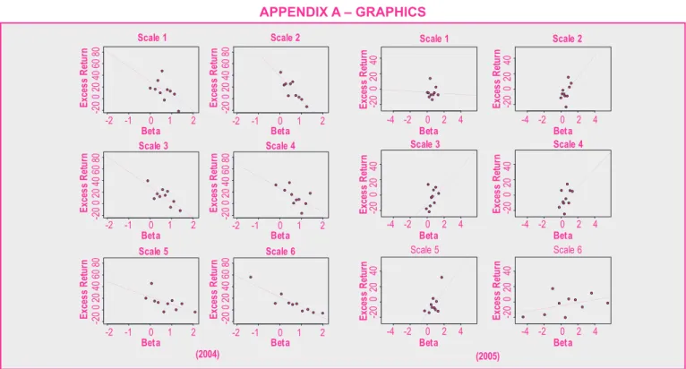
Upon analyzing the year-by-year decompositions, listed in Figures A.1 and A.2 in the Appendix, we observe the expected risk Source: Prepared by the authors using a database collected from BLOOMBERG,

2004-2007.

Note: The scales 1 to 6 correspond to the following periods: (1) 2-4 days, (2) 4-8

days, (3) 8-16 days, (4) 16-32 days, (5) 32-64 days, and (6) 64-128 days.

Figure 1: Wavelets Discrete Decomposition of Returns and Betas Average Between 2004 and 2007

E xc e ss R et ur n 0_ 10 20 30 40 E xc e ss R et ur n 0 10 20 30 40 E xc e ss R et ur n 0 10 20 30 40         Scale 1 Beta E xc e ss R et ur n

-2 0 2 4 -2 0 2 4

-2 0 2 4 -2 0 2 4 0 10 20 30 40 Scale 2 Beta E xc e ss R et ur n 0 10 20 30 40 E xc e ss R et ur n 0 10 20 30 40 Scale 3 Beta Scale 4 Beta Scale 5 Beta Scale 6 Beta Table 1

Regression of Excess Returns and Systemic Risk from 2004 to 2007 in Different Decomposition Scales

Using the Discrete Wavelet Transformation Method

Level (j) Constant Slope R²

Scale 1 0.0807** -0.0629** 0.6772

Scale 2 0.0693** -0.0459* 0.4903

Scale 3 0.0592** -0.0294 0.3648

Scale 4 0.0491 -0.0144 0.0375

Scale 5 0.0444* -0.0054 0.0180

Scale 6 0.0432** -0.0074 0.1715

Source: Prepared by the authors from a database collected from BLOOMBERG,

2004-2007.

Notes: **1% signiicance; * 5% signiicance. The constant and slope coeficients

(8)

and return relationship in 2004 and 2005 only. The expected risk and return relationship is not observed in 2006 and 2007(_*)_. In 2004, we observe a negative slope in all scales that was

signiicant at 10% for scale 1, at 1% for scales 2, 3, and 6, and

at 5% for scale 5. This is appropriate given that the historic market premium per year was -0.026 per day. The largest R2 values were obtained for scales 2, 3, and 6. However, in all the

scales, the intercept of the regression was positive. It can there-fore be concluded that in that year, the market priced systemic risk but did not do so at the magnitude predicted by the CAPM.

In 2005, the slope was negative in the irst scale but pos

-itive in the other ive scales. It was signiicant at 5% only

for scale 5, which was the scale with the greatest R2_value. The sign of the slope was as expected; the average historic market portfolio premium is 0.06%. However, the results

were signiicant only for scale 5. The constants of the regres

-sions were signiicant at 10% for scales 2, 3, and 4 and at

5% for scale 5. Therefore, it can be concluded that in that year, the estimation horizon that produced the best results

in terms of risk pricing was 32-64 days, although the mag -nitude of the premium explained by systemic risk was not as predicted by the CAPM.

Although the risk-return ratio has been observed for some years, it has not persisted along the entire time horizon, and therefore, we must reject the hypothesis that the Brazilian market has exhibited the pricing predicted by the CAPM. Other risk factors may exist beyond the market portfolio that should be taken into consideration in pricing Brazilian

assets. The literature inds evidence that size, book to mar

-ket, momentum and liquidity are signiicant factors in the

Brazilian market.

Fernandez (2006) studies the Chilean asset market and

indicates that as in the inancial market in Brazil, in which the predictions were most signiicant for the irst three scales (2-4,

4-8, and 8-16 days), the second scale (2-4 days) exhibits the

greatest coeficients of determination (even though the relation -ship predicted by the CAPM is not substantiated in his work). Thus, Fernandez concludes that the predictions of the model are more relevant in the short term. However, studies performed in other countries differ in terms of the scale that best captures the relationship between risk and returns. Gençay et al. (2003)

ind that in the American market, the model predictions are

more relevant for investors with medium and long-term time horizons, as in the United Kingdom. In Germany, on the other hand, the third scale is the most relevant (8-16 days), revealing that the medium-term horizon is the most appropriate for this

market. This may be because more mature inancial markets

possibly present a different structure for risk and returns than do less mature markets. This idea requires more in-depth study.

Rhaeim et al. (2007), in a study of the inancial market of France, observe that short and long-term horizons are the most relevant, contrary to observations in mature coun-tries such as the United States, Germany, and the United Kingdom. Aktan et al. (2009), in analyzing the assets listed

in the Istanbul stock exchange, ind a positive relationship between risk and returns that is most signiicant at the 3rd

level (8-16 days). Therefore, it is important to consider that the market analysis may differ when different time

inter-vals are studied. We should consider structural breaks and

exogenous factors not mentioned here when comparing the

inancial markets of different economies.

6. CONCLUSION

This work presents the results of the multi-scale decomposition of the assets listed in Bovespa between 2004 and 2007, using the method proposed by Gençay et al. (2003), with the goal of study -ing the relationship between systemic risk and returns for different time scales.

Our indings indicate that short term frequency produces

better estimates of betas, but we do not validate the CAPM risk return relation for the Brazilian stock market. Although the average risk premium observed during the period analyzed

was positive (7.68% per year), the estimations of the coefi -cients revealed a negative market premium for all levels of decomposition. Thus, the expected relationship between risk and returns according to the CAPM was not observed in the whole period 2004-2007.

When we investigate year by year, we observe that in 2004,

the actual market premium was negative (-6.82% per year), whereas it was positive in 2005 (16.58% per year). The observed relationship was negative for all scales for 2004 and positive

for practically all the scales except the irst in 2005, but we

did not observe the same consistency in 2006 and 2007.

We can conclude that these predictions do not apply to the

period as a whole.

Thus, keeping in mind that the estimates generated by the multi-scale decomposition model permit more robust analysis of the model for different time scales, we cannot support the hypothesis that Brazilian assets are priced according to CAPM.

The Brazilian literature identiies that other factors such as size, book-to-market, momentum and liquidity are signii

-cant in explaining Brazilian stock returns. We expect that the

inclusion of these factors in the model should improve the risk return relation. An investigation of a multifactor model based on the wavelet approach should be the objec-tive of future research. It should also be highlighted that

in order to use the wavelet approach, it was necessary for

us to ill in the days without trading in the price series with values estimated using the Kalman ilter. This step may have

generated a bias in the data, and should be considered a lim-itation of this study. 

(9)

R

EF

ER

EN

C

ES

Aktan, B., Mabrouk, A. B., Ozturk, M., & Rhaiem N. (2009). _{Wavelet-based systematic risk estimation: an application on} Istanbul stock exchange. International Research Journal of Finance and Economics, 23, pp. 33-45.

Blanchard, O. J., & Fischer, S. (1989). Lectures on macroeconomics. Cambridge: The MIT Press.

Blume, M. E. (1971, March). On the assessment of risk. Journal of Finance, 26(1), 1-10.

doi: 10.1111/j.1540-6261.1971.tb00584.x

Breeden, D. T., Gibbons, M.R., & Litzenberger, R. H. (1989). Empirical test of the consumption-oriented CAPM. The Journal of Finance, 44(2), 231-262.

doi: 10.2307/2328589

Cecco, N. M. M. (1988). A estabilidade do coeiciente beta –

uma análise empírica no mercado de ações de São Paulo. Dissertação de Mestrado, Fundação Getulio Vargas, São Paulo, SP, Brasil.

Cochrane, J. H. (1996). A cross-sectional test of an investment based asset pricing model. The Journal of Political Economy, 104(3), 572-621.

Cohen, K. J., Hawawini, G.A., Maier, S.F., Schwartz, R.A. & Whitcomb, D.K. (1983). Estimating and adjusting for the intervalling-effect bias in beta. Management Science, 29(1), 135-148.

doi: 10.1287/mnsc.29.1.135

Chui, C. K. (1992). An introduction to wavelets, wavelet analysis and its applications. San Diego, CA: Academic Press. doi: 10.1016/B978-0-12-174584-4.50005-0

Fama, E., & French, K. (1992). The cross-section of expected returns. Journal of Finance, 47(2), 427-465. doi: 10.1111/j.1540-6261.1992.tb04398.x

Fernandez, V. (2006). The CAPM and value at risk at different time-scales. International Review of Financial Analysis, 15(3), 203-219.

doi: 10.1016/j.irfa.2005.02.004

Flister, F. V., Bressan, A. A., & Amaral, H. F. (2011). CAPM conditonal no mercado brasileiro: um estudo dos efeitos momento, tamanho e book-to-market entre 1995 e 2008. Revista Brasileira de Finanças, 9(1), 105-129.

Gençay R., Whitcher B., & Selçuk, F. (2003). Systematic risk and time scales. Quantitative Finance, 3(2), 108-116. doi: 10.1088/1469-7688/3/2/305

Glenn, N., Pettengill, G. N., Sundaram, S., & Mathur, I. (1995). The conditional relation between beta and returns. The Journal of Financial and Quantitative Analysis, 30(1), 101-116. doi: 10.2307/2331255

Gregory-Allen, R., Impson, C. M., & Karaiath, I. (1994). An empirical investigation of beta stability: portfolios vs. individual securities. The Journal of Business, Finance and Accounting, 21(6), 909-916.

doi: 10.1111/j.1468-5957.1994.tb00355.x

Lakonishok, J. & Shapiro, A. (1984). Stock returns, beta, variance and size: an empirical analysis. FinancialAnalysts Journal, 40(4), 36-41.

Lima, F. G., Kimura, H., Assaf Neto, A., & Perera, L. C. J. (2010). Previsão de preços de commodities com modelos ARIMA-GARCH e redes neurais com ondaletas: velhas tecnologias – novos resultados. Revista de Administração (RAUSP), 45(2), 188-202.

Lucena, P., & Pinto, A. C. F. (2008). Anomalias no mercado de ações brasileiro: uma modiicação no modelo de Fama e French. RAC-eletrônica, 2(3), 509-530.

Lintner, J. (1965). The valuation of risky assets and the selection of risky investments in stock portfolios and capital budgets. The Review of Economics and Statistics, 47(1), 13-37.

doi: 10.2307/1924119

Machado, M. A. V., & Medeiros, O. R. (2011). Modelos de preciicação de ativos e o efeito liquidez: evidências empíricas no mercado acionário brasileiro. Revista Brasileira de Finanças. 9(3), 383-412.

Mankiw, G.N., & Shapiro, M.D. (1986). Risk and return: consumption beta versus market beta. The Review of Economics and Statistics,68(3), 452-459.

Minardi, A. m. a. f. (2004). Retornos passados prevêem retornos futuros? RAE eletrônica, 3, pp. 1-18.

doi: 10.1590/S1676-56482004000200003

Morettin, P. A. (1999). Ondas e ondaletas: análise de Fourier à análise de ondaletas. São Paulo: Edusp.

Morettin, P. A., Toloi, C. M. C., Chiann, C., & Miranda, J. C. S. (2010). Wavelet-smoothed empirical copula estimators. Revista Brasileira de Finanças, 8(3), 263-281.

Mussa, A., Trovão, R., Santos, J.O., & Famá, R. (2007). A estratégia de momento de Jagadeesh e Timan e suas implicações para a hipótese de eiciência do mercado acionário brasileiro. Anais do SEMEAD, FEA-USP, São Paulo, SP, Brasil, 10.

Ogden, R. T. (1997). Essential wavelets for statistical applications and data analysis. Boston, MA: Birkhäuser. doi: 10.1007/978-1-4612-0709-2

Oliveira, R. F., & Carrete, L.S. (2005). Estudo empírico sobre a previsibilidade do retorno de mercado no Brasil. Anais do Encontro Brasileiro de Finanças. Sociedade Brasileira de Finanças, São Paulo, SP, Brasil, 5.

Percival, D. B., & Walden, A. T. (2000). Cambridge series in statistical and probabilistic mathematics: wavelet methods for time series analysis. Cambridge, MA: Cambridge University Press.

doi: 10.1017/CBO9780511841040

(10)

R

EF

ER

EN

C

ES

Ramsey, J. B., & Lampart, C. Decomposition of economic _{relationships by time scale using wavelets.}_{Macroeconomic} Dynamics, 2(1), 49-71.

Ramsey, J. B., & Zhang, Z. (1995). The analysis of foreign exchange data using waveform dictionaries. Journal of Empirical Finance, 4, pp. 341-372.

doi: 10.1016/S0927-5398(96)00013-8

Rhaeim, N., Ammou, S.B., & Mabrouk, A. B. (2007). Wavelet estimation of systematic risk at different time scales: application to French stock market. The International Journal of Applied Economics and Finance. 1(2), 113-119.

doi: 10.3923/ijaef.2007.113.119

Reinganum, M. R. (1981). A new empirical perspective on the CAPM. Journal of Financial and Quantitative Analysis, 16, pp. 439-462.

doi: 10.2307/2330365

Roll, R., & Ross, S.A. (1995). The arbitrage pricing theory approach to strategic portfolio planning. Financial Analysts Journal, 51(1), 122-131.

Ross, S. A. (1976). The arbitrage theory of capital asset pricing. Journal of Economic Theory, 13(3), 341-360. doi: 10.1016/0022-0531(76)90046-6

Samaei, R. T. (2012). Multi scale systematic risk (an application on Tehran Stock Exchange). Journal of

Basic and Applied Scientiic Research, 2(11),

11254-11265.

Sharpe, W. (1964). Capital asset prices: a theory of market equilibrium under conditions of risk. Journal of Finance, 19(3), 425-442.

doi: 10.1111/j.1540-6261.1964.tb02865.x; doi: 10.2307/2977928

A

B

ST

R

A

C

T

R

ESU

MEN

Analysis of multi-scale systemic risk in Brazil’s inancial market

This work analyzes whether the relationship between risk and returns predicted by the Capital Asset Pricing Model (CAPM) is valid in the Brazilian stock market. The analysis is based on discrete wavelet decomposition on different time scales. This technique allows to analyze the relationship between different time horizons, since the short-term ones (2 to 4 days) up to the long-term ones (64 to 128 days). The results indicate that there is a negative or null relationship between systemic risk and returns for Brazil from 2004 to 2007. As the average excess return of a market portfolio in relation to a risk-free asset during that period was positive, it would be expected this relationship to be positive. That is, higher systematic risk should result in higher excess returns, which did not occur. Therefore, during that period, appropriate compensation for systemic

risk was not observed in the Brazilian market. The scales that proved to be most signiicant to the risk-return relation were the irst three, which corresponded to short-term time horizons. When treating differently, year-by-year, and consequently

separating positive and negative premiums, some relevance is found, during some years, in the risk/return relation predicted by the CAPM. However, this pattern did not persist throughout the years. Therefore, there is not any evidence strong enough

conirming that the asset pricing follows the model.

Keywords: stock pricing, risk-return ratio, CAPM, wavelets, Brazilian stock market.

Análisis del riesgo sistemático multiescala en el mercado inanciero de Brasil

En este trabajo se analiza si la relación entre riesgo y rendimiento prevista por el Capital Asset Pricing Model (CAPM) tiene validez en el mercado de acciones brasileño, con base en la descomposición discreta de wavelet en diferentes escalas de tiempo. Esta técnica permite analizar la relación en diferentes horizontes temporales, desde el corto plazo (2 a 4 días) hasta el largo plazo (64 a 128 días). Los resultados muestran que entre los años 2004 y 2007 existe una relación negativa o nula entre riesgo sistemático y rendimiento en Brasil. Como el rendimiento en exceso medio de la cartera de mercado sobre el activo libre de riesgo en el período fue positivo, se esperaría que esta relación fuese positiva, es decir, un mayor riesgo sistemático se traduciría en un mayor rendimiento en exceso, lo que no ocurrió. Por consiguiente, no se observó en este período una remuneración adecuada por el riesgo sistemático en el mercado brasileño. Las escalas que presentaron una

relación más signiicativa entre riesgo y rendimiento fueron las tres primeras, y corresponden a horizontes de más corto plazo.

Se puede decir que – al tratar de manera diferente año a año y, por consiguiente, separar premios positivos y negativos – se encuentra en algunos años alguna relevancia en la relación riesgo rendimiento prevista por el CAPM, pero no persiste a lo largo de todos los años. Se concluye que no hay evidencia bastante fuerte de que la valoración de los activos siga el modelo.

(11)

APPENDIX A – GRAPHICS Scale 1 Beta E xce s s R et u rn

-2 -1 0 1 2 -2 -1 0 1 2

-20 0 20 40 60 80 E

xce s s R et u rn

-20 0 20 40 60 80

Scale 2

Beta

Scale 3 Scale 4

Scale 1 Beta E xce ss R et u rn

-20 0 20 40 -20 0 20 40

Scale 2 Beta E xce ss R et u rn E xce s s R et u rn

-20 0 20 40 60 80 E

xce ss R et u rn

-20 0 20 40 Exce -20 0 20 40

ss R et u rn E xce s s R et u rn

-20 0 20 40 60 80 E

-20 0 20 40 60 80 Exce

ss

R

et

u

rn

-20 0 20 40 Exce -20 0 20 40

ss

R

et

u

rn

-4 -2 0 2 4 -4 -2 0 2 4

Beta

-2 -1 0 1 2 -2 -1 0 1 2 Beta

Beta Beta

-4 -2 0 2 4 -4 -2 0 2 4

Beta

-2 -1 0 1 2 -2 -1 0 1 2

Beta Beta Beta

-4 -2 0 2 4 -4 -2 0 2 4

Scale 5 Scale 6

(2004) (2005)

Figure A.1: Discrete Wavelet Decomposition for the Years 2004 and 2005 (Annual excess portfolio returns versus systematic risk for different levels. Scales 1 to 6 correspond to the following periods: (1) 2-4 days,

(2) 4-8 days, (3) 8-16 days, (4) 16-32 days, (5) 32-64 days, and (6) 64-128 days)

Figure A.2: Discrete Wavelet Decomposition for the Years 2006 and 2007 (Annual excess portfolio returns versus systematic risk for different levels. Scales 1 to 6 correspond to the following periods: (1) 2-4 days,

(2) 4-8 days, (3) 8-16 days, (4) 16-32 days, (5) 32-64 days, and (6) 64-128 days)

(2006) (2007) Beta E x ce s s R et u rn

-2 0 2 4 -2 0 2 4

0 20 40 60 80 100 0 20 40 60 80 100

Beta E x ce s s R et u rn Scale 3 Beta E x ce s s R et u rn Scale 4 Beta E x ce s s R et u rn Scale 5 Beta E x ce s s R et u rn Scale 6 Beta E x ce s s R et u rn Beta E x ce ss R et u rn

-1.0 -0.5 0.0 0.5 1.0 1.5 2.0 -1.0 -0.5 0.0 0.5 1.0 1.5 2.0

-2 0 2 4 -2 0 2 4 -1.0 -0.5 0.0 0.5 1.0 1.5 2.0 -1.0 -0.5 0.0 0.5 1.0 1.5 2.0

-20 0 20 40 60 -20 0 20 40 60

Beta E x ce ss R et u rn Scale 3 Beta E xc ess R et u rn Scale 4 Beta E xc ess R et u rn Scale 5 Beta E xc ess R et u rn Scale 6 Beta E xc ess R et u rn