392 Brazilian Journal of Physics, vol. 34, no. 2A, June, 2004
Compensation Temperature of the Mixed-Spin Ising
Model on the Hexagonal Lattice
W. Figueiredo, M. Godoy, and V. S. Leite
Departamento de F´ısica, Universidade Federal de Santa Catarina 88040-900, Florian´opolis, SC, Brazil
Received on 3 November, 2003
We studied a layered mixed-spin Ising model, with spinsσ = 1/2andS = 1, distributed on the sites of a hexagonal lattice. For this spin arrangement, any spin at one lattice site has two nearest-neigbor spins of the same type, and four of the other type. We assumed that the exchange interaction between spinsσandS is antiferromagnetic, with the valueJ1. J2 is the exchange interaction between two nearest neighborσspins,
andJ3 is the coupling between two nearest neighborSspins. We also considered a single-ion crystal-field
contributionDto theSsites. We performed mean-field calculations and Monte Carlo simulations to determine the compensation point of the model. We have shown that a compensation point can be present for any positive value ofD. We have also found a negative lower bound forD, below which a compensation point can not appear. For each value ofD, we determined the range of values of theJ2 andJ3 couplings for which a
compensation point is realizable.
In the recent years a lot of efforts has been dedicated to the study of the ferrimagnetic materials, specially due to their great potential for technological applications [1, 2]. The search for the new designed ferrimagnetic materials re-quires also a better understanding of their physical prop-erties. Despite their simplicity, mixed-spin Ising systems have shown to be the simplest models for studying ferri-magnetism. These models have been studied by a vari-ety of techniques, including effective-field theories [3, 4], renormalization-group calculations [5, 6, 7] and Monte Carlo simulations [8, 9].
In a ferrimagnetic material two inequivalent moments, interacting antiferromagnetically, can give rise to a zero spontaneous magnetization below its critical temperature [10]. This happens, due to the different dependences of the sublattice magnetizations on temperature. Then, a spe-cial point can appear at a temperature below the critical one, where the sublattice magnetizations cancel exactly each other. This point is the so called compensation point. The magnetic behaviour of a ferrimagnetic system near the com-pensation point is of fundamental importance in the area of the thermomagnetic recording devices [11].
The compensation temperature of a mixed-spin Ising model on the square and honeycomb lattices was already investigated. In these lattices, the nearest-neigbour interac-tions are always between spinsσandS. The mean-field ap-proximation predicts the existence of a compensation point, but only for a very narrow region of negative values of the crystal-field parameter. However, these results are in dis-agreement with Monte Carlo simulations. It is necessary to include in the simulations a next-nearest ferromagneticσ−σ
interaction, in order to have a compensation point.
In this work we investigated a layered mixed-spin Ising
model with spinsσ= 1/2andS = 1, defined on a hexago-nal lattice. The lattice is formed by alternate layers of spins
Sandσ. The hamiltonian model for this ferrimagnetic sys-tem is
H = −J1
i,j
Siσj−J2
i,j
σiσj
−J3
i,j
SiSj−D
i
S2
i, (1)
whereJ1, J2 andJ3 are the exchange couplings between nearest-neighbor pairs of spins σ−S, σ−σandS −S,
respectively, andD is the crystal-field contribution. In all the following analysis we will takeJ1 <0. We have also performed mean field calculations at the one site level. For the Monte Carlo simulations, the initial configurations were taken random, and we flipped the spins once a time, accord-ing to the heat-bath algorithm [12]. We considered hexago-nal lattices of lattice sizesL, along with periodic boundary conditions. We used lattices of sizesL= 8,16,32and64, and in each Monte Carlo step (MCs) we performedL2
tri-als of flipping the spins. In order to get reliable results, we performed around4000MCs for the lattice withL = 64, where the first1000MCs were discarded for the thermaliza-tion process. We also considered averages over100 differ-ent samples in our calculations. Although not shown in the next figures, the error bars are smaller than the symbol sizes. Then, let us present our results.
In Fig. 1, we show the behavior of the sublattice magne-tizations (mσ,mS), and of the total magnetization,mtot =
(mσ +mS)/2, as a function of the temperature. For the set of values of the exchange interactions, J1 = −1.0J,
pa-W. Figueiredo, M. Godoy, and V. S. Leite 393
rameterD =−0.75J, we observe the existence of a
com-pensation point. Fig. 1(a) shows the results of the mean-field calculations, and we foundTcomp= 0.78J/kBfor the tem-perature of the compensation point, and Tc = 1.37J/kB, for the transition temperature. As can be seen, the compen-sation point appears due to the different dependences of the sublattice magnetizations on temperature. As the tempera-ture increases, more and more spins of the sublatticeS flip from their ordered to the disordered state, because of the antiferromagnetic exchange couplingJ3. However, as the ferromagnetic exchange interaction J2 is positive, the ma-jority of the spins of the sublatticeσremains in its ordered state. AtT =Tcomp, the two sublattice magnetizations can-cel each other, giving rise to a zero total magnetization. For
T > Tcomp, the total absolute magnetization increases up to
a maximum value, and then starts to decrease, going to zero at the critical temperatureTc. Fig. 1(b), Monte Carlo simu-lations, presents the same trends of Fig. 1(a), but the results we found for the compensation and critical temperatures are
Tcomp= 0.26J/kBandTc= 0.62J/kB, respectively.
0.0 0.5 1.0 1.5 2.0
0.0 0.2 0.4 0.6 0.8 1.0
T
m
S
, m
σ
0.0 0.5 1.0 1.5 2.0
-0.05 0.00 0.05 0.10 0.15
(a)
T mtot
0.0 0.2 0.4 0.6 0.8 1.0 0.0
0.2 0.4 0.6 0.8 1.0
T
m
S
, m
σ
0.0 0.2 0.4 0.6 0.8 1.0
-0.05 0.00 0.05 0.10 0.15 0.20
(b)
T
m
tot
Figure 1. Sublattice and total magnetizations as a function of the temperature for J1 = −1.0J, J2 = 1.0J, J3 = −1.05J and
D =
−0.75J. (a) mean-field calculations and (b) Monte Carlo
simulations. The insets show the sublattice magnetizations.Tcomp
andTcare shown in the figures.
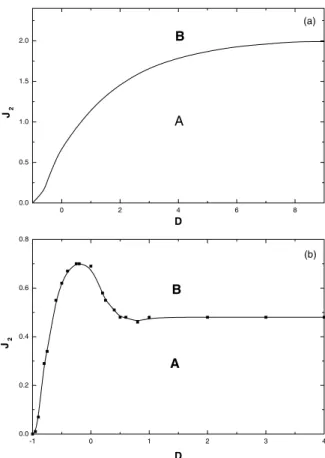
There is a minimum value of the ferromagnetic inter-action parameterJ2for the appearance of the compensation point, which depends on the value of the crystal-fieldD. We show in Fig. 2(a), the minimum value ofJ2as a function of
D in the mean-field approximation for J1 = −1.0J and
J3 =−1.0J. The minimum value ofJ2for which a com-pensation point appears is an increasing function ofD. As
D decreases, the magnetization of the sublatticeS decays faster, and the crossing point of the two sublattice magne-tizations moves to lower temperatures. At these tempera-tures, the sublatticeσis well ordered even for a small value ofJ2. In Fig. 2(b) we present the dependence ofJ2onD, obtained through Monte Carlo simulations forJ1=−1.0J andJ3=−0.98J. A different behavior appears in the range of values−0.25J < D < 0.50J, whereJ2decreases with
D. In this model, for D < −3.00J, the system is repre-sented by a set of uncoupled chains ofσspins. We attribute this behavior to a dimensional crossover, which is not cap-tured by the one site mean-field approximation.
0 2 4 6 8
0.0 0.5 1.0 1.5 2.0
(a)
B
A
D J 2
-1 0 1 2 3 4
0.0 0.2 0.4 0.6 0.8
B
A
D J 2
(b)
Figure 2. Minimum value ofJ2for the appearance of a
compensa-tion point as a funccompensa-tion of the crystal field parameterD. (a) mean-field calculations forJ1=−1.0JandJ3=−1.0, and (b) Monte
Carlo simulations forJ1 =−1.0JandJ3 =−0.98. RegionA,
ms > mσ forT < Tc, andB is the region where we have the
compensation points.
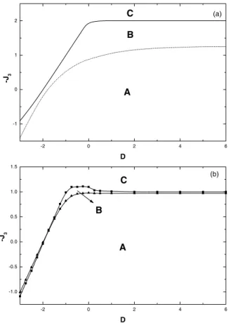
Figure 3 shows the range of values of the antiferromag-netic interactionJ3for which we have a compensation point, as a function ofD, forJ1 =−1.0J andJ2 = 1.0J. Figs. 3(a) and 3(b) give the mean-field results and Monte Carlo simulations, respectively. In these figures, we note that there is a small region of values ofJ3for which we have a com-pensation point, regionB in the figures. In the region A
we always havemS > mσ for any value ofT < Tc. On the other hand, in the regionC,mσ > mSfor any value of
394 Brazilian Journal of Physics, vol. 34, no. 2A, June, 2004
range of values forJ3. Besides, the upper-bond−J3 also exhibits a different behavior from the mean-field one in the range−0.5< D <0.
-2 0 2 4 6
-1 0 1 2
(a)
B
A C
D
-J
3
-2 0 2 4 6
-1.0 -0.5 0.0 0.5 1.0 1.5
(b)
B C
A
D -J3
Figure 3. Range of values of J3 giving rise the compensation
points, as a function of the crystal field parameterD. (a) mean-field calculations, and (b) Monte Carlo simulations.Bis the only region where we can have the compensation points. For the regions AandC, we always havems> mσ, andmσ> ms, respectively.
In summary, we presented mean-field calculations and Monte Carlo simulations for a layered mixed-spin Ising model on a hexagonal lattice. We have shown that the model can exhibit a compensation point also for positive values of
D. We have also found a negative lower bound forD, below which there is no compensation point. For each value ofD, we determined the range of values ofJ2 andJ3 where the presence of a compensation point is possible.
Acknowledgments
This work was partially supported by the Brazilian agen-cies CNPq, CNPq and FUNCITEC(SC).
References
[1] D. Gatteschi, O. Kahn, J. S. Miller and F. Palacio,Magnetic
Molecular Materials(NATO ASI Series, Kluwer Academic,
Dordrecht, 1991).
[2] H-P. D. Shieh and M. H. Kryder, Appl. Phys. Lett.49, 473 (1986).
[3] T. Kaneyoshi, Solid State Communc.70, 975 (1989); Physica A205, 677 (1994).
[4] A. F. Siqueira and I. P. Fittipaldi, J. Magn. Magn. Mater.54, 678 (1986).
[5] S. G. A. Quadros and S. R. Salinas, Physica A 206, 479 (1994).
[6] H. F. Verona de Resende, F. C. S´a Barreto and J. A. Plascak, Physica A149A, 606 (1988).
[7] J. A. Plascak, W. Figueiredo and B. C. S. Grandi, Braz. J. Phys.29, 579 (1999).
[8] G. M. Buendia and J. A. Liendo, J. Phys.: Condens. Matter.
9, 5439 (1997).
[9] G. M. Buendia, M. A. Novotny and J. Zhang. Springer Proceedings in Physics. Computer Simulation Studies in Condensed-Matter Physics VII. Eds. D. P. Landau, K. K. Mon and H. B. Sch¨uttler. Springer-Verlag, 223-227 (1994).
[10] L. N´eel, Ann. de Phys.3, 137 (1948).
[11] M. Mansuripur, J. Appl. Phys.61, 1580 (1987).
[12] D. P. Landau and K. Binder,A Guide to Monte Carlo
Sim-ulations in Statistical Physics(Cambridge University Press,