Individual and Aggregate Money Demands

Individual and Aggregate Money Demands

∗

André C. Silva

Nova School of Business and Economics

July 2011

Abstract

I construct a model in which money and bond holdings are consistent with individual decisions and aggregate variables such as production and interest rates. The agents are infinitely-lived, have constant-elasticity preferences, and receive a fraction of their income in money. Each agent solves a Baumol-Tobin money management problem. Markets are segmented becausefinancial frictions make agents trade bonds for money at different times. Trading frequency, consumption, government decisions and prices are mutually consistent. An increase in inflation, for example, implies higher trading frequency, more bonds sold to account for seigniorage, and lower real balances.

JEL Codes: E3, E4, E5.

Keywords: money demand, cash management, inventory problem, market segmentation.

1. Introduction

Aggregate variables such as the money-income ratio depend on individual decisions.

Here, I combine the general equilibrium Baumol-Tobin models of Jovanovic (1982)

and Romer (1986) with the market segmentation models of Grossman and Weiss

(1983), Rotemberg (1984), and Grossman (1987) to connect individual decisions to

variables used in monetary policy. The objective is to create a framework to analyze

consumption, prices, and money taking into account the changes in the individual

demands for money.

I use two features from the models above. I obtain the demands for money from

an inventory model of Baumol (1952) and Tobin (1956) in general equilibrium, as

Jo-vanovic and Romer (other general equilibrium Baumol-Tobin models are in Fusselman

and Grossman 1989, Heathcote 1998, Chiu 2007, and Rodriguez-Mendizabal 2006).

And I express individual optimization problems as in the market segmentation models

of Grossman and Weiss, and Rotemberg. As a result, agents trade bonds for money

at different times, now with the trading frequency obtained in equilibrium.

In addition to combining the two frameworks, I make two changes from the models

above. First, the model has infinitely-lived agents and consumption smoothing while

Jovanovic assumes constant consumption and Romer assumes zero intertemporal

dis-count and overlapping generations. I consider consumption smoothing because it

affects the demand for money and the welfare cost of inflation. Infinite-lived agents,

on the other hand, remove the influence of the length of life of each generation on

equilibrium variables. In particular, consumption and money over time after policy

changes are not affected by the length of each generation. Infinite lives and

consump-tion smoothing, moreover, facilitate comparison with cash-in-advance models such as

the models of Lucas and Stokey (1987), and Cooley and Hansen (1989, 1991).

allow a fraction of income in money because market segmentation implies large holding

periods to match data on velocity (Edmond and Weill 2008), holding periods of six

months or larger. As traditional Baumol-Tobin models implicitly assume that agents

receive their income in interest-bearing bonds (Karni 1973), large holding periods

would make agents separated from their income for a long period. Therefore, I follow

Alvarez et al. (2009) and Khan and Thomas (2010) and assume that agents receive

part of their income in bonds and the remaining in money. The fraction of income

in money is thought to be substantial, sixty percent for example, and interpreted as

labor income.

The result is a monetary model in which trading periods, consumption and the

distribution of money holdings are consistent with individual decisions and aggregate

variables. An increase in inflation, for example, implies higher trading frequency,

more bonds sold to account for seigniorage, and lower real balances. Silva (2009,

forthcoming) uses the model to study the effects of interest rate shocks and the

welfare cost of inflation. Even with the modifications made here, the model allows its

steady state to be characterized analytically.

Having the frequency of trades chosen optimally, as in the model, implies a better

fit with the data on money and interest rates. The demand for money, for example,

has an interest elasticity of −0.5 and semi-elasticity of −12.5. The interest

elastic-ity is approximately zero, in contrast, with fixed holding periods (Romer 1986 and

Grossman 1987). The choice of the interval between trades makes easier for agents

to change their demand for money.

2. The Model

There is a continuum of infinitely-lived agents with measure one. There is an asset

market and a goods market. The asset market concentrates trades between bonds

Only money can be used to buy goods. The government sets government consumption

and taxes and controls the supply of money through open market operations.

The financial frictions appear when agents transfer resources between the asset

market and the goods market. Each agent has a brokerage account and a bank

account, as in Alvarez et al. (2002, 2009). The brokerage account is used to manage

the activities in the asset market and the bank account to manage the activities in the

goods market. Thefinancial frictions are represented by a transfer costΓin real terms

that the agents need to pay whenever they transfer resources between the brokerage

account and the bank account. The transfer cost is paid with the resources in the

brokerage account and it does not depend on the volume transferred. Γ represents a

fixed cost of portfolio adjustment.

Time is continuous, t _≥ 0. Time is continuous to avoid integer constraints on

the decision of the time to make transfers. At t = 0, each agent has M0 in money

in the bank account and B0 in bonds in the brokerage account. There is a given

distribution F of M0 and B0. Index agents by their initial holdings of money and

bonds, s= (M0, B0).

Each agent is composed of three participants, a worker, a trader, and a shopper,

as in Lucas (1990). At the beginning of each period, the worker engages in the

production and sales of the consumption good, the trader goes to the asset market

to manage the brokerage account, and the shopper goes to the goods market to buy

consumption goods. At the end of each period, the three participants rejoin to share

the consumption good.

The flow of funds occurs in the following way. The worker produces Y (t) goods

and sells the production for money to other agents in the goods market by the price

P (t). After the sale, the worker transfers aP(t)Y (t) to the bank account and

(1₋a)P(t)Y (t) to the brokerage account. The trader trades bonds and money

traders or with the government in open market operations. If it is necessary to make

a transfer from the brokerage account to the bank account, the trader sells the

neces-sary quantity of bonds and makes the transfer. In the same way, the trader can make

transfers from the bank account to the brokerage account. As the money deposited

in the brokerage account cannot be used to buy goods and does not receive interest,

the money in the brokerage account is immediately used to buy bonds. The shopper

uses the available money in the bank account to buy goods in the goods market.

The shopper then brings the goods purchased to the other participants to be shared

among then in the end of the period.

In Baumol (1952) and Tobin (1956), the agents have access to money only when

they pay the financial costs to convert bonds into money. This case is obtained here

with a = 0. Then, all sales are converted into bonds and the shopper can only use

the sales proceeds to buy goods after a transfer from the brokerage account to the

bank account. The introduction of a fraction a >0 allows the shopper to use part of

the sales proceeds immediately. To simplify, the transfers of the worker to the trader

and to the shopper do not pay the financial costs. Only the transfers between the

brokerage account and the bank account pay the financial costs.

Agentsdecides consumptionc(t, s), the times to make transfersTj(s),j = 1,2, ...,

money and bond holdings in the bank and brokerage account, M(t, s), B(t, s), and

the transfers of money between the two accounts,z(t, s). The worker, the trader, and

the shopper are together represented as agent s. Let T0(s)≡0. T0 is not a decision

variable. If an agent decides to make the first transfer at t = 0, then T1(s) = 0. A

holding period is given by (Tj, Tj+1).

Letr(t) denote the nominal interest rate at time t. If there is not a transfer at t,

bond holdings in the brokerage account evolve as

˙

wherex˙ is the derivative ofxwith respect to time. If there are no transfers, the agent

simply accumulates the interest rate and the income from sales. Bond holdings in the

brokerage account increase.

Let B−_(T

j(s), s) represent bond holdings just before a transfer at t = Tj and

B+_(T

j(s), s)represent bond holdings just after the transfer,B−(Tj(s), s)≡limt→Tj,

t<TjB(t, s) andB+(Tj(s), s)≡limt→Tj,t>TjB(t, s). At t=Tj, the constraint on the

brokerage account is

z(Tj(s), s) +P (Tj(s))Γ=B−(Tj(s), s)−B+(Tj(s), s), t=T1(s), T2(s), ... (2)

If there is a positive transfer to the bank account, z(Tj(s), s)>0, thenB−(Tj(s), s)

> B+_(T

j(s), s). In this case, bond holdings in the brokerage account decrease just

after the transfer.

Money holdings in the bank account follow

˙

M(t, s) =₋P (t)c(t, s) +aP(t)Y (t), t_≥0, t6=T1(s), T2(s), ..., (3)

during a holding period. If there are no transfers, money holdings decrease with goods

purchases and increase with the income transfers from sales. The shopper can use the

money transferred from the worker to buy goods in the same period. Analogously

to the definitions for bond holdings, let M+_(T

j(s), s) and M−(Tj(s), s) denote

money holdings just after a transfer and money holdings just before a transfer. We

have z(Tj(s), s) = M+(Tj(s), s)−M−(Tj(s), s). If the transfer is positive then

M+_(T

j(s), s)−M−(Tj(s), s)>0. When there is a transfer,

˙

M(Tj(s), s)+=−P (Tj)c+(Tj(s), s) +aP(t)Y (t),t ≥0, t=T1(s), T2(s), ...,

(4)

andc+_(T

j(s), s) is consumption just after the transfer. Notice that the government

does not distribute money directly to agents with, for example, lump-sum transfers.

Only those agents in the asset market, trading bonds for money, have access to the

transfers of money from the government.

The agents make transfers so thatM+_(T

j(s), s) covers the purchases during (Tj,

Tj+1) and any balanceM−(Tj+1(s), s), that is, using (3),

M+(Tj(s), s) =

Z Tj+1(s)

Tj(s)

P (t)c(t, s)dt₋

Z Tj+1(s)

Tj(s)

aP(t)Y (t)dt+M−(Tj+1(s), s),

(5)

j = 1,2, ...Agents= (M0, B0)starts withM0 in money holdings att= 0. The agent

has to useM0 until thefirst transfer, atT1(s). For thefirst holding period (0, T1(s)),

we have

M0 =

Z T1(s)

0

P(t)c(t, s)dt−

Z T1(s)

0

aP(t)Y (t)dt+M−(T1(s), s). (6)

It can be the case that the agent chooses to make the first transfer at t = 0. For

example, if a= 0 andM0 = 0. In this case, T1(s) = 0, and M−(0, s) = 0.

Let Q(t) denote the price at time zero of a bond that pays one dollar at time t.

Given the nominal interest rate r(t), Q(t) =e−R(t)_{, where R(t) =}Rt

0r(τ)dτ. Using

(1), Q(Tj+1)B−(Tj+1) = Q(Tj)B+(Tj) +R_TjTj+1Q(t) (1−a)P Y (t)dt. Substituting

for the different holding periods, together with the conditionlimt→∞Q(t)B(t) = 0,

we obtain the constraint on the brokerage account in present value,

∞

X

j=1

Q(Tj(s)) [z(Tj(s), s) +P(Tj(s))Γ]≤

Z ∞

0

Q(t) (1₋a)P (t)Y (t) +B0, (7)

The problem of agents is then to obtain c(t, s),M(t, s), and Tj(s) to solve

max ∞

X

j=0

Z Tj+1(s)

Tj(s)

e−ρt_{u(c(t, s))dt (8)}

subject to (3)-(7) and to Tj+1(s) ≥ Tj(s) and M(t, s) ≥ 0. ρ is the intertemporal

rate of discount. The utility function isu(c) = c₁1₋−₁1_//_ηη,η 6= 1,η >0; andu(c) = logc, η = 1. The transfer cost does not enter in the utility function. η is the elasticity of

intertemporal substitution.

It is never optimal to set M−_(T

j+1) > 0, j ≥ 1. M−(Tj+1) > 0 means that

the agent maintained money holdings in the bank account during the whole holding

period (Tj, Tj+1) without receiving interest. The agent is always better off reducing

the amount transferred at Tj, M+(Tj+1), until M−(Tj+1) = 0. As agents cannot

change M0, it can still be the case that M−(T1)>0. For the other holding periods,

M−(Tj+1) = 0. Therefore, using (3), the demand for money at t of agent s is given

byM(t, s) =RTj+1(s)

t [P (t)c(t, s)−aP(t)Y (t)]dt, Tj(s)≤t < Tj+1(s), j ≥1.

The transfer cost rules out an equilibrium with a representative agent. In a standard

cash-in-advance model, agents have access to bonds and to their income in the end of

every period. Here, agents have access to their bonds and to their income deposited

in bonds only when they sell bonds for money. At every moment, some agents sell

part of their bonds for money and make a transfer while others accumulate bonds

and keep using money in the bank account until the next transfer.

To make the budget constraints linear in income, let Γ = γY (t). As preferences

are homothetic, this implies that optimal consumption and that the demand for

money are linear in income. A demand for money linear in income, that is, income

elasticity equal to one, agrees with the empirical evidence as discussed, among others,

by Meltzer (1963), Lucas (2000).

LetBG

with no taxes and no government consumption. In this case, all seigniorage collected

by the government is redistributed to agents as initial bonds. The government budget

constraint is BG

0 =

R∞

0 Q(t)P(t)

˙

M(t)

P(t)dt, whereM(t)is the aggregate money supply.

Higher money growth implies higherBG

0 and more bonds distributed across agents.

The market clearing conditions for money and bonds areM(t) =R M(t, s)dF(s)

andBG

0 =

R

B0(s)dF(s). The market clearing condition for goods takes into account

the goods used to pay the transfer cost. Let A(t,δ)≡{s :Tj(s)∈ [t, t+δ]} denote

the set of agents that make a transfer during [t, t+δ]. The number of goods during

[t, t+δ] to pay the transfer cost is then given byR_A(t,δ)1_δΓdF(s). Taking the limit to obtain the number of goods used at time t yields that the market clearing condition

for goods is given by Rc(t, s)dF(s) + limδ_→0R_A(t,δ)1_δΓdF(s) =Y.

An equilibrium is defined as pricesP (t),Q(t), allocationsc(t, s),M(t, s), transfer

times Tj(s), j = 1,2, ..., and a distribution of agentsF such that (i)c(t, s),M(t, s),

andTj(s)solve the maximization problem (8) givenP (t)andQ(t)for allt≥0ands

in the support ofF; (ii) the government budget constraint holds; and (iii) the market

clearing conditions for money, bonds, and goods hold.

Solving the model

Focus on the steady state, an equilibrium in which the nominal interest rate is

constant at r, the inflation rate is constant at π, and aggregate consumption grows

at the same rate of output. Let output grow at the rate g, Y (t) = Y0egt, where ρ>

g(1−1/η). I look for an equilibrium in which all agents have the same consumption

pattern within holding periods and the same interval between transfers N. The

steady state is interpreted as the allocations and prices of an economy that has not

been exposed to shocks for a long time.

Rewrite the maximization problem in terms of the consumption-income ratioˆc(t, n)

≡c(t, n)/Y (t). ˆc(t, n)decreases at a constant rate within holding periods, according

value at the beginning of a holding period. With the exception of the short holding

period from t = 0 to the first transfer, let the steady state be such that all agents

begin a holding period with the same consumption-income ratio, ˆc0.

At a certain timet,ˆc(t, n) varies across agents because each agent is in a different

position in the holding period. But all agents look the same within holding periods.

They start with the same consumption-income ratio and it decreases at a common

rate. As the maximization problem can be written in terms of the

consumption-income ratio, having the same ˆc0 implies that all agents choose the same interval

between transfers N. Let n represent the time of the first transfer, n ∈ [0, N).

Therefore, an agent nmakes transfers at n, n+N and so on.

As aggregate consumption grows at the same rate of aggregate output, the same

number of agents must be starting a new holding period at every time. Otherwise,

aggregate consumption would vary over time. As a result, the distribution of agents

is uniform along[0, N), with density1/N.1

Thefirst order condition with respect to consumption impliesc(t, n) = _[P0e_Q−₍(ρ+π)η_T t

j)λ(n)]η,

t _∈ (Tj, Tj+1), j = 1,2, ..., using P(t) = P0eπt, and where λ(n) is the Lagrange

multiplier of (7). Set the nominal interest rate in the steady state atr=ρ+g/η+π.

The first order condition then implies c˙(t, n)/c(t, n) = ₋ηr +g and that ˆc(t, n)

decreases at the rate ηr.

Ifη, r or a are high, then agents would consume more in the beginning of holding

periods by borrowing against their money receipts within the same holding period.

They would consume less thanaY in the end of a holding periods. A useful property

of the model is that c > aY for the empirically relevant range of η, r, and a. That

is, for η between zero and five, r between zero to 16% per year, and a _≤ 0.6. This

is the empirically relevant range of η, r, and a because the usual estimates of η are

below five (Bansal and Yaron 2004 and Bansal 2006 discuss the evidence about η,

Bansal and Yaron focus onη= 1.5); the annual interest rate for the U.S. is below16%

during 1900-1997, using commercial paper rate forr; and because money receipts are

interpreted as labor income, implyinga _≤0.6(Khan and Thomas 2010 and Alvarez et

al. 2009 also interpret money receipts as labor income; I use the same value forathat

they use,a= 0.6). We can, therefore, study the properties of the equilibrium without

the constraint c≥ aY. This property facilitates the analysis and characterization of

the equilibrium.

The value of ˆc0 is obtained with the market clearing condition for goods. The

market clearing condition for goods implies 1

N

RN

0 cˆ(t, n)dn +

γ

N = 1. Write the

consumption-income ratio within holding periods as ˆc(t, n) = ˆc0e−ηr(t−Tj(n)), for the

highest j(n) such that Tj(n) ≤ t < Tj+1(n). The market clearing holds for every

t. In particular, for t = N, 1

N

RN

0 ˆc0e−ηr(N−n)dn+

γ

N = 1, which implies ˆc0(N) = ¡

1_{− N}γ¢ ³1−e−ηrN

ηrN

´−1

.

The effect of the transfer cost is apparent in the term γ/N. As we must take

into account γ/N, the consumption-income ratio can be less than1 during the entire

holding period. With transfer cost in utility terms, γ/N disappears and cˆ0 > 1.

The effect of γ through the market clearing condition would not be considered. The

expression of N, given in proposition 1 below, implies N >γ. So, cˆ0 >0.

The first order conditions forTj(n), j = 2,3, ..., imply

(r−π−g)γ +r

Z Tj+1

Tj

e(π+g)(t−Tj)ˆc(t, n)dt+£cˆ+(Tj, n)−erNˆc−(Tj, n)¤

= cˆ

+_(T

j, n)−erNˆc−(Tj, n)

1−1/η +r

Z Tj+1

Tj

ae(π+g)(t−Tj)_dt+a¡_1−erN¢_{. (9)}

The left hand side and the right hand side are the marginal gain and loss of delaying

decreasing balances from Tj to Tj+1; the third term is the net effect of increasing

[Tj−1, Tj) and decreasing [Tj, Tj+1), this effect is zero when η = 1. The right hand

side is given by the loss in utility caused by the increase inTj, and by the net effect of

the money receipts within the holding period. We obtainN with (9), r=ρ+g/η+π,

and the expression of ˆc(t, n).

Proposition 1 The optimal interval between transfers N is the positive root of

ˆ

c0(N)rN

∙

1₋e−r(η−1)N

r(η−1)N −

1₋e−[ρ−g(1−1/η)+r(η−1)]N

[ρ−g(1−1/η) +r(η−1)]N

¸

= [ρ₋g(1₋1/η)]γ

+arN

∙

erN ₋₁

rN −

e[r−ρ+g(1−1/η)]N ₋₁

[r₋ρ+g(1₋1/η)]N

¸

, for η6= 1, and (10)

ˆ

c0(N)rN

∙

1₋1−e− ρN

ρN

¸

=ργ+arN

∙

erN ₋₁

rN −

e(r−ρ)N ₋₁

(r₋ρ)N

¸

, for η= 1, (11)

whereρ> g(1−1/η) and ˆc0(N) =¡1−_Nγ¢ ³1−e

−ηrN

ηrN

´−1

. N exists and is unique for

all positive a that satisfies ˆc0e−ηrN ≥a and all positive values of γ, η, ρ,g, andr.

With the value of N, we find all optimal trading periods Tj(n), n ∈ [0, N), as

agents trade at n, n+N and so on. Withγ in utility terms, cˆ0 disappears fora = 0

from (10) and (11). As discussed above, cˆ(t) _≥ a (and so cˆ0e−ηrN ≥ a) for the

empirically relevant cases.

The formulas were arranged to facilitate the identification of the terms1−e−x

x ≈1−

x

2

andex_x−1 ≈1+x₂, wherex≥0in the formulas ifη≥1,π ≥0, andg ≥0. In particular,

ρ₋g(1₋1/η) +r(η₋1) = rη₋π₋g andr₋ρ+g(1₋1/η) =π+g.

Proposition 2 N is such that (i) ∂N

∂r <0 and (ii)

∂N

∂γ >0. Moreover, (iii) ∂N

∂a >0;

(iv) ∂_∂ρN > 0; (v) ∂_∂ηN > 0 if g = 0; ∂_∂ηN > 0 if g > 0 for η > ηg, where ηg is given in

the proof of the proposition; and (vi) ∂N

∂g <0 if η>1 and

∂N

Proposition 2 shows that N decreases withr and increases with γ. In addition,N

increases withaandρ. Wheng = 0,N increases withη, and wheng >0,N increases

with η ifη is sufficiently high, and decreases withη if η is close to zero. The familiar

substitution and income effects are present in the model. They have opposite signs

and cancel each other when η = 1: N increases with g if η < 1, decreases if η >1,

andg disappears from the formula of N if η = 1.

The parameters that affectN the most arer,γ and a. To see this, make a

second-order expansion of (10). The result is N _≈ p2γ/(ˆc0(N)−a)r. The Baumol-Tobin

model assumes a = 0 and constant c = Y (so ˆc0 = 1). In this case, the

square-root formulap2γ/r approximates the optimalN. The square-root formula does not

approximate N when a > 0. With a = 0.6, for example, and ˆc0(N) = 1 (a good

approximation for cˆ0 when r is small such as 3%), we have N ≈

p

2γ/(0.4r) =

1.6p2γ/r, 60% higher than the square root approximation. Money receipts within

holding periods increase the interval between transfers. For a given a, in any case,

the interest elasticity ofN is close to−0.5.

With the value ofN, the output growth rateg, and the fact that agents consume at

the rate−ηr+g within holding periods, we obtain M0(n)andW0(n) such that the

economy is in the steady state fromt = 0 and on. The growth rateg is used to write

consumption just after a transfer. The consumption-income ratioˆc0 at the beginning

of holding periods aftert=T1(n)is the same for all agents in the steady state. The

value ofˆc(0, n)differs across agents because the holding period that initiates att = 0

has different lengths, according to n _∈ [0, N). We have c+_(T

j(n), n) = ˆc0Y0egTj(n):

consumption at the beginning of holding periods grows at the rate g. Proposition 3

gives the values ofM0(n). As we don’t needB0(n)to discuss the demand for money,

the values of B0(n) are in the proof of proposition 3, in the appendix.

Proposition 3 The initial money holdings such that the economy is in a steady state

equilibrium for t ≥ 0 are given by M0(n) = P0Y0n[eηr(n−N)cˆ01−e

ae[r−ρ+g(1−1/η)]n₋₁

[r−ρ+g(1−1/η)]n ], n∈[0, N), where cˆ0(r, N) = ¡

1_{− N}γ¢ ³1−e−ηrN

ηrN

´−1

and N is given

by proposition (1).

An agent withM0(n)makes transfers att=n, n+N, and so on. Asˆc0e−ηrN > a,

M0(n) increases with n. So, agents that make the first transfer later have more

initial money holdings. Analogously, the initial value in the brokerage accountB0(n)

decreases withn. If an agent makes thefirst trade of bonds for money soon (nsmall),

then B0(n)is high.

Although the distribution of agents along[0, N)is uniform, with densityf(n) = 1

N,

the distribution of individual money holdings is not uniform. As prices and output

grow over time, individual money holdings also grow over time. So, consider the

distribution of individual money-income ratios. The distribution of money-income

ratios is constant over time.

The individual money-income ratio is given by b(n) = M0(n)

P0Y0 . The individual

money-income ratio is distributed along [0, mH), where mH = limn→Nb(n). The

density fb(m) of the individual money-income ratios is given by f(b−1(m))∂b

−1_(m)

∂m ,

where f(n) = 1

N and b−

1_{(m) is the value of n such that b(n) = m (as b(n) is}

in-creasing, we always have one and a unique value of b−1_{(m)). Therefore, f}

b(m) =

1

N[ηrm+e

[r−ρ+g(1−1/η)]b−1_(m)

(ˆc0e−ηrN −a) +ηrae

(r−ρ+g(1−1/η))b−1(m)₋₁

[r−ρ+g(1−1/η)] ]−

1_{, m ∈[0, m}

H).

The distribution of real money holdings is concentrated on small quantities of money,

but it is close to a uniform. The distribution is more concentrated on small quantities

of money if η increases.2

We obtain the aggregate demand for money with M0 = _N1

RN

0 M0(n)dn. The

aggregate money-income ratio m(r), the inverse of velocity, is obtained by dividing

M0 byP0Y0. The aggregate money-income ratio is then

m(r) = ˆc0(r, N)e −ηrN

ρ−g(1−1/η) +r(η−1)

∙

eηrN ₋₁

ηrN −

e[r−ρ+g(1−1/η)]N ₋₁

[r−ρ+g(1−1/η)]N

¸

− a

r−ρ+g(1−1/η)

∙

e[r−ρ+g(1−1/η)]N ₋₁

[r−ρ+g(1−1/η)]N −1

¸

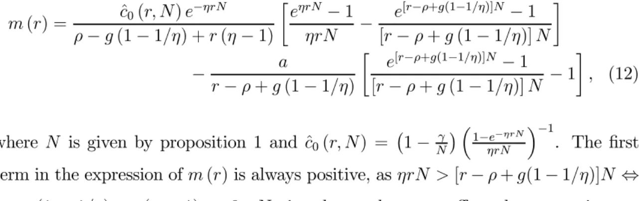
, (12)

where N is given by proposition 1 and ˆc0(r, N) = ¡1−_Nγ¢ ³1−e

−ηrN

ηrN

´−1

. The first

term in the expression ofm(r)is always positive, asηrN >[r−ρ+g(1−1/η)]N ⇔

ρ ₋g(1₋ 1/η) + r(η ₋1) > 0. Notice that g does not affect the money-income

ratio if η = 1. A fractiona of income received directly as money means, in practice,

that the agents need to hold less money to buy goods. So, m decreases witha. The

aggregate money-income ratio is a function of the interest raterand also of preference

parameters, financial technology, and output growth. I write m(r) to emphasize the

relation of the money-income ratio to the interest rate.

Figure 1 shows m(r) and U.S. annual data. I use M1 for money and commercial

paper rate for r, as Lucas (2000), Lagos and Wright (2005) and others (there are

questions about the choice of the proxies for M andr, as pointed out by Teles and

Zhou 2005, I use M1 and commercial paper rate to facilitate comparison with the

lit-erature). A second-order approximation ofm(r)yields(e−ηrN_cˆ

0−a)N₂. The interest

elasticity of m is, therefore, close to the interest elasticity of N, −0.5. Lucas (2000)

argues that an interest elasticity of₋0.5provides a goodfit to the data. Many

empir-ical studies, however,find smaller interest elasticities in absolute value, especially for

the short-run. More recently, on the other hand, Alvarez and Lippi (2009) estimate

interest elasticities close to −0.5. The semi-elasticity of m is −12.5, compatible with

the findings of Lucas (1988), Stock and Watson (1993), and the long-run elasticities

of Guerron-Quintana (2009).

0 2 4 6 8 10 12 14 16 0.1 0.15 0.2 0.25 0.3 0.35 0.4 0.45 0.5 0 1 2 3 45 6 7 8 9 10 11 12 13 14 15 16 17 18 19 20 21 22 23 24₂₅ 26 27 28 29 30 31 32 33 34 35 36 37 38 39 40 41 42 4344 45 46 47 4849 50 51₅₂ 53 54 55 56 57 58 59 60 61 6263₆₄ 65 66 67 68 69 70 71 72 73 74 75 7677 ₇₈ 79 80 81 82 83 84 85 8687 88 89 90 91 92 93 94 95 96 97 M o n e y -i nc om e ra ti o , m (r)

Nominal interest rate (% p.a.)

Fig. _{1. m(r) and U.S. data, 1900-1997 (M1/(PY) for the money-income ratio and}

commercial paper rate for the nominal interest rate, the data points indicate years).

η = 1 (log utility). I set a = 0.6, as Alvarez et al. (2009) and Khan and Thomas

(2010), who interpret a as labor income. The only parameter left is γ, which I set

to γ = 1.265%. γ is set so that m(r) passes through the historical average of the

data, that is, m(¯r) equals the historical money-income ratio whenr¯is the historical

interest rate, obtained with their geometric means. This is the same procedure of

Lucas (2000). Similarly, Alvarez et al. (2009) and Khan and Thomas (2010) calibrate

their models tofit the historical M2 velocity.

γ = 1.265% means that agents in the model spend about 22 minutes per week in

financial transfers when inflation is equal to 1%. To get this value, notice that γ/N

is the cost of financial transfers per year as a fraction of income. When π = 1%,

proposition 1 implies that N = 1.27. With the average weekly hours from 1957 to

1997 of U.S. workers, equal to 36.5 according to the OECD, the time devoted to

The model implies a large interval between transfers, as common in market

seg-mentation models (Edmond and Weill 2008). With π = 1%, g = 2%, and a= 0, the

model impliesN of about 6months. N increases to1.27year when a= 0.6. Alvarez

et al. (2009), for example, set the transfer interval from 1.5 to 3 years (larger

inter-vals because they use M2). Financial transfers both here and in Alvarez et al. are

transfers from high-yielding assets to currency, not ATM withdrawals, which change

the allocations of checking deposits and currency, but do not change the quantity of

money. Although large, the transfer intervals agree with the low trading frequency of

households (Vissing-Jorgensen 2002, Alvarez et al. 2009) and the large cash holdings

of firms (Bates et al. 2009). Notice that agents in the model represent households

andfirms, as62% of M1 in the U.S. is held byfirms (Bover and Watson 2005). Silva

(forthcoming) discusses the calibration in more detail and comparesm(r)witha = 0

or0.6, N fixed or optimal, and differentη’s.

I simplified the model to facilitate its application: the objective is to create a

framework to study changes in monetary policy taking into account the frictions

to manage money holdings and a nondegenerate distribution of money holdings. In

particular,m(r)is stable with constantγand constantfinancial market participation.

Following Reynard (2004) we can obtain a stable m(r) with decreasing γ (financial

innovation) together with increasing financial market participation. It simplifies,

however, to have constant γ and financial market participation. As figure 1 shows,

these assumptions imply a close match with the data. Another simplification is to

impose that agents need money to buy goods through a cash-in-advance constraint

instead of obtaining a demand for money from matching as in Kiyotaki and Wright

(1989), Rocheteau and Wright (2005), and Lagos and Wright (2005). Moreover,

Mulligan and Sala-i-Martin (2000) and Ireland (2009) point out that the demand

for money changes with low interest rates. The model is intended to be used with

follow the general pattern of the data.

With taxes and government consumption, the government budget constraint

changes to

B0+

Z ∞

0

Q(t)P (t)Gdt=

Z ∞

0

Q(t)τdt+

Z ∞

0

Q(t)M˙ S(t)dt, (13)

where G is government consumption and τ is a lump-sum tax. The total supply of

government bonds is still given byB0 = _N1 R B0(n)dn. With lump-sum taxes andaas

the fraction in money of gross income, each agent transfers to the brokerage account

R∞

0 Q(t) [P (t) (1−a)Y (t)−τ]dt at each time. According to (13), if revenues from

seigniorage are zero, for example, then B0 =

R∞

0 Q(t) [τ −P (t)G]dt, which means

that net government revenues are rebated to agents through government bonds.

Different ways offinancing government consumption, therefore, affect the economy

in different ways. A higher G financed with an increase in τ decreases consumption

to satisfy the market clearing condition for goods, but does not change the frequency

of trading bonds for money. According to (13), this is done by making the increase in

τ equal to the increase inG so thatM˙S_{(t)does not change. As} M˙

M =π+g, inflation

and the decision onN do not change.

On the other hand, an increase in G financed with seigniorage increases inflation.

The change in inflation implies an additional decrease in consumption because the

frequency of trading increases and so the resources devoted to financial transactions

increase. In a model withfixedN, financingGwith taxes or seigniorage would yield

similar results. Seigniorage would still increase inflation, but the effect on

consump-tion would be restricted to consumpconsump-tion smoothing within holding periods. Here, the

3. Conclusions

This paper introduces a model to study how changes in monetary policy such as

changes in the interest rate or in the money supply affect prices and the real demand

for money. The distribution of money holdings, prices, interest rates, production and

government actions are consistent in equilibrium. That is, they are consistent with

market clearing conditions, budget constraints and individual maximization.

The model combines the Baumol-Tobin general equilibrium frameworks of

Jo-vanovic (1982) and Romer (1986) with the market segmentation models of Grossman

and Weiss (1983) and Rotemberg (1984). The result is a cash-in-advance model in

which the length of the time period is optimal and money holdings are heterogeneous.

Some applications of the model are to study how changes in the trading frequency

affect the demand for money and the welfare cost of inflation. Taking into account

the changes in the trading frequency, Silva (forthcoming) shows that the estimates of

the welfare cost of inflation increase substantially. More generally, the model is useful

to study how the adjustment of money holdings affects real variables.

Appendix - Proofs

I will use the following functions and definitions in propositions 1, 2 and 3: f(x) =

1−e−x

x , ˆρ ≡ ρ −g(1− 1/η), x1 ≡ r(η−1)N, x2 ≡ x1 + ˆρN, g(y) = ey₋₁

y , y1 =

rN, y2 = y1 − ˆρN. ˆρ > 0 by assumption to imply a bounded solution for the

maximization problem, sox2 > x1 andy1 > y2. Moreover,g is increasing and convex

and so [g(y1)−g(y2)] > 0 and [g0(y1)−g0(y2)] > 0, as y1 > y2. Similarly, f is

decreasing and convex and so [f(x1)−f(x2)] > 0 and [f0(x1)− f0(x2)] < 0, as

x1 < x2. LetG be defined byG(N) = ˆc0(N)rN[f(x1)−f(x2)]−ˆργ−z(N), where

z(N) =arN[g(y1)−g(y2)]. The optimal interval N∗ is such thatG(N∗) = 0.

e−ρTj_u(c−_(T

j))−e−ρTju(c+(Tj))−λ[Q˙ (Tj)

RTj+1

Tj P (t)c(t)dt+Q(Tj)P (Tj)c

+_(T

j)

−Q(Tj−1)P(Tj)c−(Tj)+Q˙ (Tj)R_TjTj+1aP(t)Y egtdt−Y egTjP (Tj)a(Q(Tj)−Q(Tj−1))

−γY egTj_(P(T

j)Q˙ (Tj) +Q(Tj)P˙ (Tj))−YγgegTjP (Tj)Q(Tj)] = 0. The first order

conditions for consumption yield e−ρTj_c−_(T

j)−1/η = λQ(Tj−1)P (Tj) and e−ρTj ×

c+_(T

j)−1/η = λQ(Tj)P(Tj). In the steady state, Q(t) = e−rt and P(t) = P0eπt,

Nj = N, and c(t) = ˆc(t)Y0egt. Substituting and simplifying yields γ(r −π−g) +

£

ˆ c+_(T

j)−erNcˆ−(Tj)

¤

= ˆc+(Tj)₁−₋e₁rN_/ηcˆ−(Tj)−rRTj+1

Tj

ˆ

c(t)e(g+π)

e(g+π)Tj dt +r

RTj+1

Tj

ae(g+π)t

e(g+π)Tjdt+a(1−

erN_{). Moreover, ˆc(t) = ˆc}

0e−ηr(t−Tj), ˆc+(Tj) = ˆc0, and erNcˆ−(Tj) = e−r(η−1)Ncˆ0.

Substituting yieldscˆ01−e

−r(η−1)N

η−1 −rˆc0

RTj+1

Tj e

(g+π−ηr)(t−Tj)_{dt= (r−π−g)γ+a(e}rN₋

1)₋raRTj+1

Tj e

(g+π)(t−Tj)_{dt. Solving the integrals and rearranging yields (10). Note}

that r=ρ+g/η+π. The steps for η= 1 are analogous.

For existence and uniqueness, the strategy is to show thatGis increasing inN, with

limN→γG(N)<0 and limN→+∞G(N)>0. These three properties ofG imply that N∗ _{exists and is unique. MoreoverN}∗ _{>γ. We haveG(r, N) = ˆc}

0(N) [1−e

−r(η−1)N

η−1 −

r1−e_ρˆ−₊[ˆρ+_r(ηr(η₋−₁₎1)]N]−ˆργ−a[erN _−1−re(r−ˆρ)N₋₁

r−ˆρ ]and so GN = ˆc0NrN[f(x1)−f(x2)] + rerN_(1−e−ˆρN_)[ˆc

0(N)e−ηrN − a]. If a = 0 then, as cˆ0N ≡ ∂ˆc0(N)/∂N > 0, we

have GN > 0. If a > 0 then a sufficient condition for GN > 0 is cˆ0(N)e−ηrN ≥ a.

That is, consumption in the end of a holding period is higher than or equal to the

money receipts. This condition is satisfied because of the constraintc(t, n)≥aY (t).

As discussed in the text, in any case, we always have c(t, n) > aY (t), nonbinding,

for the empirically relevant parameters. For η = 1, analogously, GN > 0. For the

limits, we have limN→+γGN(N) ≤ −ˆργ for all η > 0, with equality if and only if

a = 0. So, limN→+γGN(N) < 0. Finally, limN→+∞GN(N) > 0 for all η > 0.

Therefore, limN→+∞G(N) = +∞. (Eventually, the constraint ˆc(t) ≥ a binds, as limN→+∞ˆc0(N)e−ηrN = 0; we still have in this case that limN→+∞G(N) = +∞.)

Therefore, G crosses the zero and, as it is increasing, it crosses the zero only once.

Proposition 2. Proof. We have to obtain the sign of ∂_∂N_x = −GGxN((NN∗∗)) to prove

each property, whereGis defined above andGx denotes∂G/∂x. In proposition 1, we

already proved that GN >0.

(i) ∂N

∂r < 0. We have to show that Gr(N∗) > 0. Consider first the case a = 0.

We have Gr = ˆc0N[f(x1)−f(x2)]h(x1), using ˆc0r = −ˆc0f

0_(rηN)

f(rηN)ηN, and where

h(x1) = 1−rηNf

0_(rηN)

f(rηN) +r(η−1)N

f0_(x2)−f0_(x1)

f(x2)−f(x1) . Ifη<1, all terms in the expression

of h(x1) are positive and so Gr > 0 (recall that f0 < 0, f0(x2)−f0(x1) > 0 and

f(x2)−f(x1) < 0). The same reasoning applies for η = 1. For η > 1, notice that

x1 ≡r(η−1)N >0and writeh(x1)ash(x) = 1−(x+rN)f

0_(x+rN)

f(x+rN)+x

f0_(x+ρN)−f0_(x) f(x+ρN)−f(x) ,

x > 0. The function xf_f0₍(_xx₎) is decreasing (so ₋(x+rN)f_f0₍(_xx₊+_rNrN₎) > ₋xf_f0₍(_xx₎)) and we have f_f0₍(x_x+₊ρ_ρN_N)₎₋−f_f0₍(_xx₎) > f_f000₍(_xx₎). Therefore, h(x) > 1−x

f0_(x)

f(x) +x

f00_(x)

f0_(x), which is positive for allx. As a result, Gr >0.

When a > 0, we have Gr = ˆc0N[f(x1)−f(x2)]h(x1)−zr(N), where zr(N) >

0. Substituting the definition of z(N), we obtain that Gr > 0 if and only if a <

ˆ

c0[f(x1)−f(x2)]h(x1)

[g(y1)−g(y2)]+rN[g0(y1)−g0(y2)]. In practice (for a ≤0.6 and the standard values forη and r, for example), this condition is always satisfied and so Gr>0.

(ii) ∂_∂γN >0. Gγ =−rf(x1)−f(x2)]

f(rηN) −ˆρ<0.

(iii) ∂N

∂a >0. Ga=−rN[g(y1)−g(y2)]<0.

(iv) ∂_∂ρN >0. It suffices to show thatGˆρ<0, as ρˆ=ρ−g(1−1/η). We haveGˆρ=

−ˆc0rN2f0(x2)−γ−arN2g0(y2). Fora = 0,Gˆρ(N∗)<0ifˆc0rN2f0(x2)>−γ atN∗,

which is true because−γ = ˆc0rN2f(x2)_ρˆ−_Nf(x1) when N =N∗, andf0(x2)> f(x2)_ˆρ−_Nf(x1),

as f is convex. Therefore, Gˆρ<0. Whena increases, Gˆρ decreases as the first order

effect onGˆρis−rN2g0(y2)<0(the effect ofN onGˆρ, caused by the increase in a, is

small compared with the first order effect of a). Therefore, Gρˆ(N∗) is also negative

for a >0.

(v) ∂N

∂η > 0. We have to prove that Gη < 0. For g = 0, Gη = ˆc0(rN)

2

[f(x1)−

f(x2)]h(x1), using cˆ0η = −ˆc0f

0_(rηN)

f(rηN)rN, and where h(x1) =

f0_(x2)−f0_(x1) f(x2)−f(x1) −

So Gη < 0 if h(x1) < 0 (the condition is the same for a ≥ 0). Write h(x1) as

h(x) = f_f0(₍x_x+₊ρ_ρN_N))−₋f_f0₍(_xx₎) ₋ f_f0₍(_xx₊+_rNrN₎), x > ₋rN. We have f_f0₍(x_x+₊ρ_ρN_N)₎₋−f_f0₍(_xx₎) < f_f000₍(_xx₊+_ρρ_NN₎) and f00_(x+ρN)

f0_(x+ρN) <

f0_(x+ρN)

f(x+ρN). Therefore, h(x)<

f0_(x+ρN)

f(x+ρN) −

f0_(x+rN)

f(x+rN). Ifr > ρ then

f0_(x+ρN) f(x+ρN) <

f0_(x+rN)

f(x+rN) as

f0_(x)

f(x) is increasing. So, h(x)< 0 and Gη < 0. If r < ρ, use the fact that

f0_(y)−f0_(x)

f(y)−f(x) is increasing in y and so

f0_(x+ρN)−f0_(x)

f(x+ρN)−f(x) < limρN→∞

f0_(x+ρN)−f0_(x) f(x+ρN)−f(x) =

f0_(x) f(x).

Therefore,h(x)< f_f0₍(_xx₎)₋f_f0₍(_xx₊+_rNrN₎) <0as f_f0₍(_xx₎) is increasing. So,h(x)<0andGη <0. When g > 0, we have Gη = ˆc0(rN)2h(x1) +rNgN_η2 ˆc0[f0(x2)− f(x2)_ˆρ−_Nf(x1)] for a = 0

(the idea is similar for a > 0). The second term in the right in positive because

f0_(x

2)> f(x2)_ˆρ−_Nf(x1). We have Gη > 0 for η close to zero when g > 0. Let ηg >0 be

such that Gη¡η_g¢= 0. Therefore, Gη <0 if and only if η>η_g.

(vi) ∂_∂N_g < 0 if η > 1 and ∂_∂N_g > 0 if η < 1. The only term in which g appears is

ˆ

ρ=ρ₋g(1₋1/η), ∂N/∂ˆρ>0. As ∂ˆρ/∂g =₋(η₋1)/η, ∂N/∂g has the same sign

of ∂N/∂ˆρ if η < 1 and the opposite sign if η >1 (g disappears from the formula of

N if η= 1).¥

Proposition 3. Proof. M0(n) is such that agent nconsumes at the steady state

rate in the interval[0, n),M0(n) =R₀nP(t)c(t, n)dt−R₀naP(t)Y0egtdt. Agentn= 0

consumesc0 at timet = 0. Given that the consumption growth rate within N in the

steady state is equal to₋(ηr₋g), and that consumption just after a transfer grows

at the rate g, an arbitrary agent n consumes c0e−ηr(N−n) at t = 0. That is, agent n

would consumec0e−gNegn att=n−N <0and consumes¡c0e−gNegn¢e−(ηr−g)(N−n)=

c0e−ηr(N−n) at t = 0. Therefore, c(t, n) = c0e−ηr(N−n)e−(ηr−g)t, 0 ≤ t < n.

More-over, P (t) = P0eπt in the steady state. Substituting above and solving the

inte-grals yields the value of M0(n) in the body of the text. For W0, let W0(n) ≡

R∞

0 Q(t) (1−a)P (t)Y (t)+B0(n). Then,W0(n)is such thatW0(n) =

P∞

j=1Q(Tj)×

M+_(T

j(n)) + P∞j=1Q(Tj)P (Tj)γY (t), equal to the present value of future

trans-fers plus transfer costs. The quantity of money needed in each holding period

M+_(T

c0egTj(n)e−(ηr−g)(t−Tj) and Tj(n) = n+ (j−1)N. Substituting and solving yields

P∞

j=1Q(Tj)M+(Tj(n)) = P0Y0N e

−(ρ−g(1−1/η))n

1−e−(ρ−g(1−1/η))N [ˆc0f(x2)−ag(y2)]. Similarly, we have

P∞

j=1Q(Tj)P (Tj)γY (t) = P0Y0γe

−(ρ−g(1−1/η))n

1−e−(ρ−g(1−1/η))N . Initial bond holdings B0(n) can then

be obtained with the definition ofW0(n).¥

References

Alvarez, Fernando, Andrew Atkeson, and Chris Edmond (2009). “Sluggish

Responses of Prices and Inflation to Monetary Shocks in an Inventory Model of Money

Demand.” Quarterly Journal of Economics, 124(3): 911-967.

Alvarez, Fernando, Andrew Atkeson, and Patrick J. Kehoe (2002). “Money,

Interest Rates, and Exchange Rates with Endogenously Segmented Markets.”Journal

of Political Economy, 110(1): 73-112.

Alvarez, Fernando, and Francesco Lippi (2009). “Financial Innovation and

the Transactions Demand for Cash.” Econometrica, 77(2): 363-402.

Bates, Thomas W., Kathleen M. Kahle, and Rene M. Stulz (2009). “Why

Do U.S. Firms Hold so Much More Cash than They Used to?” Journal of Finance,

64(5): 1985-2021.

Bansal, Ravi, and Amir Yaron (2004). “Risks for the Long Run: A Potential

Resolution of Asset Pricing Puzzles.” Journal of Finance, 59(4): 1481-1509.

Bansal, Ravi (2006). “Long Run Risks and Risk Compensation in Equity

Mar-kets.” In R. Mehra (ed.), Handbook of Investments: Equity Risk Premium. North

Holland: Amsterdam.

Baumol, William J. (1952). “The Transactions Demand for Cash: An Inventory

Theoretic Approach.” Quarterly Journal of Economics, 66(4): 545-556.

Berentsen, Aleksander, Gabriele Camera and Christopher Waller (2004).

“The Distribution of Money and Prices in an Equilibrium with Lotteries.”Economic

Bover, Olympia, and Nadine Watson (2005). “Are There Economies of Scale in

the Demand for Money by Firms? Some Panel Data Estimates.”Journal of Monetary

Economics, 52(8): 1569-1589.

Chiu, Jonathan (2007). “Endogenously Segmented Asset Market in an Inventory

Theoretic Model of Money Demand.” Bank of Canada Working Paper 2007-46.

Edmond, Chris, and Pierre-Olivier Weill (2008). “Models of the Liquidity

Effect.” In S. N. Durlauf and L. E. Blume (eds), The New Palgrave Dictionary of

Economics, 2nd Edition. Palgrave Macmillan.

Fusselman, Jerry and Sanford J. Grossman (1989). “Monetary Dynamics with

Fixed Transaction Costs.” Princeton University Working Paper.

Grossman, Sanford J. (1985). “Monetary Dynamics with Proportional

Trans-action Costs and Fixed Payment Periods.” National Bureau of Economic Research,

Working Paper 1663.

Grossman, Sanford J. (1987). “Monetary Dynamics with Proportional

Transac-tion Costs and Fixed Payment Periods.” InNew Approaches to Monetary Economics,

ed. W. Barnett, and K. Singleton, 3-41. New York: Cambridge University Press.

Grossman, Sanford J. and Laurence Weiss (1983). “A Transactions-Based

Model of the Monetary Transmission Mechanism.”American Economic Review, 73(5):

871-880.

Guerron-Quintana, Pablo A. (2009). “Money Demand Heterogeneity and the

Great Moderation.”Journal of Monetary Economics, 56(2): 255-266.

Heathcote, Jonathan (1998). “Interest Rates in a General Equilibrium

Baumol-Tobin Model.” Working Paper.

Ireland, Peter N. (2009). “On the Welfare Cost of Inflation and the Recent

Behavior of Money Demand.” American Economic Review, 99(3): 1040-1052.

Jovanovic, Boyan (1982). “Inflation and Welfare in the Steady State.” Journal of

Karni, Edi (1973). “The Transactions Demand for Cash: Incorporation of the

Value of Time into the Inventory Approach.” Journal of Political Economy, 81(5):

1216-1225.

Khan, Aubhik, and Julia K. Thomas (2010). “Inflation and Interest Rates with

Endogenous Market Segmentation.” Working Paper.

Kiyotaki, Nobuhiro, and Randall Wright (1989). “Money as a Medium of

Exchange.” Journal of Political Economy, 97(4): 927-954.

Lagos, Ricardo, and Randall Wright (2005). “A Unified Framework for

Mone-tary Theory and Policy Analysis.” Journal of Political Economy, 113(3): 463-484.

Lucas, Robert E., Jr. (1988). “Money Demand in the United States: a

Quanti-tative Review.”Carnegie-Rochester Conference Series on Public Policy, 29: 137-168.

Lucas, Robert E., Jr. (1990). “Liquidity and Interest Rates.” Journal of

Eco-nomic Theory, 50: 237-264.

Lucas, Robert E., Jr. (2000). “Inflation and Welfare.” Econometrica, 68(2):

247-274.

Lucas, Robert E., Jr. and Nancy Stokey (1987). “Money and Interest in a

Cash-in-Advance Economy.”Econometrica, 55(3): 491-513.

Meltzer, Allan H. (1963). “The Demand for Money: Evidence from the Time

Series.”Journal of Political Economy, 71(3): 219-246.

Mulligan, Casey B., and Xavier Sala-i-Martin (2000). “Extensive Margins

and the Demand for Money at Low Interest Rates.” Journal of Political Economy,

108(5): 961-991.

Reynard, Samuel (2004). “Financial Market Participation and the Apparent

In-stability of Money Demand.”Journal of Monetary Economics, 51(6): 1297-1317.

Rocheteau, Guillaume, and Randall Wright (2005). “Money in Search

Equi-librium, in Competitive EquiEqui-librium, and in Competitive Search Equilibrium.”

Rodriguez-Mendizabal, Hugo (2006). “The Behavior of Money Velocity in High

and Low Inflation Countries.”Journal of Money, Credit and Banking, 38(1): 209-228.

Romer, David (1986). “A Simple General Equilibrium Version of the

Baumol-Tobin Model.” Quarterly Journal of Economics, 101(4): 663-686.

Rotemberg, Julio J. (1984). “A Monetary Equilibrium Model with Transactions

Costs.” Journal of Political Economy, 92(1): 40-58.

Santos, Manuel S. (2006). “The Value of Money in a Dynamic Equilibrium

Model.”Economic Theory, 27(1): 39-58.

Silva, Andre C. (2009). “Prices and Money after Interest Rate Shocks with

En-dogenous Market Segmentation.” Working Paper.

Silva, Andre C. (forthcoming). “Rebalancing Frequency and the Welfare Cost of

Inflation.”American Economic Journal: Macroeconomics.

Stock, J., and Watson, M. (1993). “A Simple Estimator of Cointegrating Vectors

in Higher Order Integrated Systems.” Econometrica, 61(4): 783-820.

Teles, Pedro, and Ruilin Zhou (2005). “A Stable Money Demand: Looking

for the Right Monetary Aggregate.”Economic Perspectives, Federal Reserve Bank of

Chicago, 29(1st Quarter): 50-63.

Tobin, James (1956). “The Interest-Elasticity of the Transactions Demand for