Title:
Valuing an Offshore Exploration Project Through Real
Options Analysis
Field of study:
Finance
Purpose:
Dissertation for obtaining the Degree of Master in Business
Administration (The Lisbon MBA International)
Author:
Pedro Santos
Thesis
Supervisor:
Professor José Corrêa Guedes
Abstract
This thesis applied real options analysis to the valuation of an offshore oil exploration project, taking into consideration the several options typically faced by the management team of these projects. The real options process is developed under technical and price uncertainties, where it is considered that the mean reversion stochastic process is more adequate to describe the movement of oil price through time. The valuation is realized to two case scenarios, being the first a simplified approach to develop the intuition of the used concepts, and the later a more complete case that is resolved using both the binomial and trinomial processes to describe oil price movement.
Acknowledgements
I would like to thank my thesis supervisor, Professor José Corrêa Guedes, for his guidance and advises, and whose support helped me achieve the completion of this thesis. I would also like to thank Professors Gary Emery and Pedro Santa Clara for their recommendations, and Galp Energia, Daniel Elias, and Catarina Ceitil for their help and accessibility in providing the required project information and data.
Contents
Introduction ... 1
1. Literature Review ... 3
2. Data Sources and Methods Used to Collect Data ... 6
3. Oil and Gas Exploration Decision Taking Process ... 7
4. Real Options Analysis ... 13
5. Oil Price Stochastic Process ... 15
5.1. Estimating Mean Reversion Parameters ... 17
6. Approach to Project Resolution... 19
7. Simplified Case ... 22
8. Complete Case ... 32
8.1. Sensitivity Analysis to Project Parameters ... 34
8.2. Options Value ... 39
Conclusions ... 41
References ... 42
Appendix A – Bayesian Analysis ... 48
Appendix B – Real Options Taxonomy ... 49
Appendix C – Geometric Brownian Motion ... 51
Appendix D – Trinomial Tree Building Procedure ... 52
Appendix E – Simplified Case Technological Uncertainty Project Data ... 56
Appendix F – Simplified Case Price Uncertainty Project Data ... 57
Appendix G – Effect of New Information (Simplified Case) ... 69
Appendix H – Simplified Case End Nodes Free Cash Flows Estimation ... 71
Appendix I - Simplified Case Hexanomial Tree Probabilities ... 81
Appendix J– Simplified Case ROA Tree Evolution ... 85
Appendix K – Complete Case Technological Uncertainty Project Data ... 86
Appendix L – Complete Case Price Uncertainty Project Data ... 88
Appendix M- Effect of New Information (Complete Case) ... 94
Appendix N – Oil Price Evolution from End Nodes ... 96
Appendix O – Production Levels ... 98
Appendix P – Complete Case End Nodes Free Cash Flows Estimation (Trinomial) ... 101
Appendix Q – Complete Case End Nodes Free Cash Flows Estimation (Binomial) ... 124
Appendix R – Complete Case Hexanomial Tree Probabilities ... 126
Appendix S – Complete Case Quadranomial Tree Probabilities ... 133
Appendix U – Quadranomial Tree Mutually Exclusive NPVs ... 138
Appendix V – Complete Case Real Option Analysis ... 141
Appendix W – Effects of Varying Project Volatility ... 143
Appendix X – Real Options Analysis at the Absolute Certainty Level ... 144
Appendix Y – Real Options Analysis with DW2 Having a Cost of $50 Million ... 147
Nomenclature
DCF - Discounted Cash Flow ... 1
DW - Delineation Well ... 22
GBM - Geometric Brownian Motion ... 15
LP - Large Platform ... 7
MAD - Market Asset Disclaimer ... 4
MRM - Mean Reversion Model ... 16
PV - Present Value ... 24
ROA - Real Options Analysis ... 1
SEK - Standard Error for Kurtosis ... 60
SES - Standard Error for Skewness ... 60
List of Figures
Figure 1 Oilfield Development Decision Tree ... 8
Figure 2 Oilfield Development Decision Tree with Computational Results ... 10
Figure 3 Sensitivity Analysis to Readapting Costs from a Small Platform to a Large Platform ... 11
Figure 4 Sensitivity Analysis to New Data Being Sufficient to Determine Quantity of Oil .... 11
Figure 5 Sensitivity Analysis to the Initial Probability of Having a Large Quantity of Oil ... 12
Figure 6 Sensitivity Analysis to the Cost of Purchasing Additional Information ... 12
Figure 7 Average Crude Oil Price Evolution (Data source: World Bank) ... 15
Figure 8 GBM and MRM Variance Evolution (Source: Dias, 2004) ... 16
Figure 9 Quadranomial Possible Outcomes ... 20
Figure 10 Call Option Value ... 20
Figure 11 Hexanomial Tree Outcomes and Call Option Value ... 21
Figure 12 Simple Case Oilfield Development Decision Tree ... 22
Figure 13 Simple Case Hexanomial Event Tree ... 23
Figure 14 Acquiring Additional Imperfect Information NPV ... 26
Figure 15 NPV for Setting a Large Platform at Year One ... 27
Figure 16 NPV for Setting a Small Platform at Year One ... 28
Figure 17 Real Options Analysis NPV ... 29
Figure 18 Real Options Analysis Process... 30
Figure 19 Complete Case Oilfield Development Decision Tree ... 32
Figure 20 Sensitivity Analysis to Oil Price Volatility (Value of Flexibility) ... 34
Figure 21 Sensitivity Analysis to Oil Price Volatility (Project Value) ... 35
Figure 22 Sensitivity Analysis to the Sufficiency of DW2 Data ... 35
Figure 23 Sensitivity Analysis to the Cost of Acquiring New Information ... 36
Figure 24 Sensitivity Analysis to the Initial Probability of Large Quantity of Oil ... 37
Figure 25 Sensitivity Analysis to the Initial Probability of Small Quantity of Oil ... 37
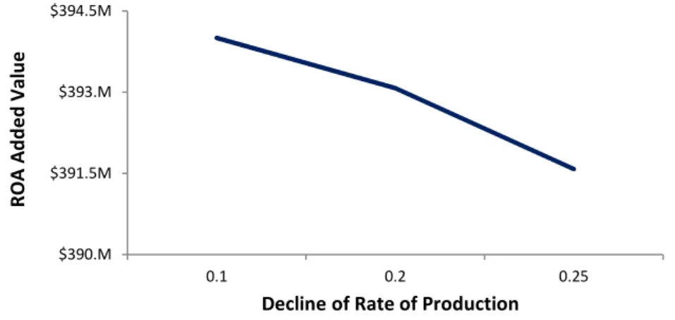
Figure 26 Sensitivity Analysis to the Decline of the Rate of Production ... 39
Figure 27 Trinomial Tree Branching Alternatives ... 53
Figure 28 Tree for X* in Hull-White Model (First Stage) ... 54
Figure 29 Crude Oil Price Evolution ... 58
Figure 30 Plot of Residuals versus X ... 59
Figure 31 Plot of Residuals versus Predicted Y ... 59
Figure 32 Residuals Normal Probability Plot ... 61
Figure 34 Price Evolution Trinomial Tree Nodes ... 65
Figure 35 Effect of New Information to Technological Uncertainty Decision Tree (Simplified Case) ... 70
Figure 36 Real Options Analysis Process... 85
Figure 37 Price Evolution Trinomial Tree Nodes ... 89
Figure 38 Effect of New Information to Technological Uncertainty Decision Tree (Complete Case) ... 95
Figure 39 Price Evolution when Deciding to Set a Large or a Small Platform at Year Three 97 Figure 40 Price Evolution when Deciding to Set a Large or a Small Platform at Year Four .. 97
Figure 41 Production Levels for Set Large at Year Three ... 98
Figure 42 Production Levels for Large Quantity of Oil ... 99
Figure 43 Production Levels for Small Quantity of Oil ... 100
Figure 44 Evolution of Year Four Price Levels ... 124
Figure 45 Evolution of Year Five Price Levels ... 124
Figure 46 Complete Case Hexanomial Event Tree... 135
Figure 47 Acquiring Additional Imperfect Information NPV (Hexanomial) ... 136
Figure 48 NPV for Setting a Large Platform at Year Three (Hexanomial) ... 137
Figure 49 NPV for Setting a Small Platform at Year Three (Hexanomial) ... 137
Figure 50 Complete Case Quadranomial Event Tree ... 138
Figure 51 Acquiring Additional Imperfect Information NPV (Quadranomial) ... 139
Figure 52 NPV for Setting a Large Platform at Year Three (Quadranomial) ... 140
Figure 53 NPV for Setting a Small Platform at Year Three (Quadranomial) ... 140
Figure 54 Hexanomial Tree Real Options Analysis ... 141
Figure 55 Quadranomial Tree Real Options Analysis ... 142
Figure 56 Hexanomial Tree Real Options Analysis ... 144
Figure 57 Quadranomial Tree Real Options Analysis ... 145
Figure 58 Hexanomial Tree Real Options Analysis ... 147
Figure 59 Quadranomial Tree Real Options Analysis ... 148
Figure 60 Hexanomial Tree Real Options Analysis (initial large oil probability at 40%) .... 150
Figure 61 Quadranomial Tree Real Options Analysis (initial large oil probability at 40%) . 151 Figure 62 Hexanomial Tree Real Options Analysis (initial large oil probability at 70%) .... 152
Figure 63 Quadranomial Tree Real Options Analysis (initial large oil probability at 70%) . 153 Figure 64 Hexanomial Tree Real Options Analysis (initial large oil probability at 100%) .. 154
List of Tables
Table 1 Considered States of Nature ... 9
Table 2 Probabilities in Case New Data Indicates the Presence of a Large Amount of Oil ... 9
Table 3 Probabilities in Case New Data Indicates the Presence of a Small Amount of Oil ... 9
Table 4 Joint Probabilities Addition ... 10
Table 5 Effect of a value increase on the variables ... 14
Table 6 Best Option without Real Options Analysis ... 28
Table 7 Real Options Analysis Added Value ... 31
Table 8 Best Option without Real Options Analysis ... 33
Table 9 Best Option with Real Options Analysis ... 33
Table 10 Individual Option Value ... 39
Table 11 Total Value of Used Options ... 40
Table 12 Simplified Case Technological Uncertainty Project Data ... 56
Table 13 Crude Oil Price (Source: World Bank) ... 57
Table 14 Used Data Set Regression Results ... 58
Table 15 Results of Kurtosis and Skew Statistical Tests ... 60
Table 16 Results from the Durbin-Watson Test ... 62
Table 17 Estimation of Mean Reversion Parameters through Linear Regression... 63
Table 18 Crude Oil Price Logarithmic Returns ... 63
Table 19 Volatility Estimation through Logarithmic Price Returns ... 64
Table 20 Input Parameters for the Construction of the Trinomial Tree ... 64
Table 21 Tree Modulation Parameters ... 64
Table 22 j Tree ... 65
Table 23 Table for X* and Nodes Probabilities ... 66
Table 24 Spot Average Crude Oil Futures Prices (Source: World Bank) ... 66
Table 25 Tree for Q ... 67
Table 26 Q Values ... 67
Table 27 αααα Values ... 67
Table 28 Trinomial Tree for Oil Prices ... 68
Table 29 Considered States of Nature ... 69
Table 30 Probabilities in Case New Data Indicates the Presence of a Large Amount of Oil . 69 Table 31 Probabilities in Case New Data Indicates the Presence of a Small Amount of Oil . 69 Table 32 Joint Probabilities Addition ... 69
Table 33 Oil Estimated Quantities and States of Nature Probabilities ... 71
Table 35 Set Small Platform – Free Cash Flow Estimates for Large Amount of Oil ... 72
Table 36 Set Small Platform – Free Cash Flow Estimates for Small Amount of Oil ... 72
Table 37 Buy Additional Information, Data Indicates Large Quantity, Large Platform is Established – Free Cash Flow Estimates for Large Amount of Oil ... 73
Table 38 Buy Additional Information, Data Indicates Large Quantity, Large Platform is Established – Free Cash Flow Estimates for Small Amount of Oil ... 74
Table 39 Buy Additional Information, Data Indicates Large Quantity, Small Platform is Established – Free Cash Flow Estimates for Large Amount of Oil ... 75
Table 40 Buy Additional Information, Data Indicates Large Quantity, Small Platform is Established – Free Cash Flow Estimates for Small Amount of Oil ... 76
Table 41 Buy Additional Information, Data Indicates Small Quantity, Large Platform is Established – Free Cash Flow Estimates for Large Amount of Oil ... 77
Table 42 Buy Additional Information, Data Indicates Small Quantity, Large Platform is Established – Free Cash Flow Estimates for Small Amount of Oil ... 78
Table 43 Buy Additional Information, Data Indicates Small Quantity, Small Platform is Established – Free Cash Flow Estimates for Large Amount of Oil ... 79
Table 44 Buy Additional Information, Data Indicates Small Quantity, Small Platform is Established – Free Cash Flow Estimates for Small Amount of Oil ... 80
Table 45 Simplified Case Hexanomial Tree Nodes Probabilities ... 81
Table 46 Complete Case Technological Uncertainty Project Data ... 86
Table 47 Input Parameters for the Construction of the Trinomial Tree ... 88
Table 48 Tree Modulation Parameters ... 88
Table 49 j Tree ... 89
Table 50 Table for X* and Nodes Probabilities ... 90
Table 51 Spot Average Crude Oil Futures Prices (Source: World Bank) ... 91
Table 52 Tree for Q ... 91
Table 53 Q Values ... 92
Table 54 αααα Values ... 92
Table 55 Trinomial Tree for Oil Prices ... 93
Table 56 Input Parameters for the Construction of the Binomial Tree ... 93
Table 57 Calculated Parameters for the Construction of the Binomial Tree ... 93
Table 58 Binomial Tree for Oil Prices ... 93
Table 59 Considered States of Nature ... 94
Table 60 Probabilities in Case New Data Indicates the Presence of a Large Amount of Oil . 94 Table 61 Probabilities in Case New Data Indicates the Presence of a Small Amount of Oil . 94 Table 62 Joint Probabilities Addition ... 94
Table 65 Production Levels for Set Large at Year Three ... 98
Table 66 Production Levels for Large Quantity of Oil ... 99
Table 67 Production Levels for Small Quantity of Oil ... 100
Table 68 Oil Estimated Quantities and States of Nature Probabilities ... 101
Table 69 Set Large Platform at Year Three – Position s3L Q NPV Estimate ... 102
Table 70 Set Large Platform at Year Three End Nodes NPV Estimates ... 103
Table 71 Set Small Platform at Year Three – Position s3SO Q NPV Estimate ... 104
Table 72 Set Small Platform at Year Three – Quantity is Large End Nodes NPV Estimates 105 Table 73 Set Small Platform at Year Three – Position s3S§ Q NPV Estimate ... 106
Table 74 Set Small Platform at Year Three – Quantity is Small End Nodes NPV Estimates 107 Table 75 Buy information at Year Three, Large Quantity is Indicated, Large Platform is Set, it is Large – Position s3b(D+)LO X NPV Estimate ... 108
Table 76 Buy information at Year Three, Large Quantity is Indicated, Large Platform is Set, Quantity is Large – End Nodes NPV Estimates ... 109
Table 77 Buy information at Year Three, Large Quantity is Indicated, Large Platform is Set, it is Small – Position s3b(D+)L§ X NPV Estimate ... 110
Table 78 Buy information at Year Three, Large Quantity is Indicated, Large Platform is Set, Quantity is Small – End Nodes NPV Estimates ... 111
Table 79 Buy information at Year Three, Large Quantity is Indicated, Small Platform is Set, it is Large – Position s3b(D+)SO X NPV Estimate ... 112
Table 80 Buy information at Year Three, Large Quantity is Indicated, Small Platform is Set, Quantity is Large – End Nodes NPV Estimates ... 113
Table 81 Buy information at Year Three, Large Quantity is Indicated, Small Platform is Set, it is Small – Position s3b(D+)S§ X NPV Estimate ... 114
Table 82 Buy information at Year Three, Large Quantity is Indicated, Small Platform is Set, Quantity is Small – End Nodes NPV Estimates ... 115
Table 83 Buy information at Year Three, Small Quantity is Indicated, Large Platform is Set, it is Large – Position s3b(D-)LO X NPV Estimate ... 116
Table 84 Buy information at Year Three, Small Quantity is Indicated, Large Platform is Set, Quantity is Large – End Nodes NPV Estimates ... 117
Table 85 Buy information at Year Three, Small Quantity is Indicated, Large Platform is Set, it is Small – Position s3b(D-)L§ X NPV Estimate ... 118
Table 86 Buy information at Year Three, Small Quantity is Indicated, Large Platform is Set, Quantity is Small – End Nodes NPV Estimates ... 119
Table 87 Buy information at Year Three, Small Quantity is Indicated, Small Platform is Set, it is Large – Position s3b(D-)SO X NPV Estimate ... 120
Table 89 Buy information at Year Three, Small Quantity is Indicated, Small Platform is Set,
it is Small – Position s3b(D-)SO X NPV Estimate ... 122
Table 90 Buy information at Year Three, Small Quantity is Indicated, Small Platform is Set, Quantity is Small – End Nodes NPV Estimates ... 123
Table 91 Project Year Four NPVs ... 125
Table 92 Project Year Five NPVs ... 125
Table 93 Complete Case Hexanomial Tree Nodes Probabilities ... 126
Table 94 Complete Case Quadranomial Tree Nodes Probabilities ... 133
Table 95 Project Results with Oil Price Standard Deviation at Ten Percent ... 143
Table 96 Project Results with Oil Price Standard Deviation at Twenty Percent ... 143
Table 97 Project Results with Oil Price Standard Deviation at Fifty Percent ... 143
Table 98 Best Option with Real Options Analysis ... 146
Table 99 Best Option with Real Options Analysis ... 149
Table 100 Best Option with Real Options Analysis (initial large oil probability at 40%) .... 156
Table 101 Best Option with Real Options Analysis (initial large oil probability at 70%) .... 156
Table 102 Best Option with Real Options Analysis (initial large oil probability at 100%) .. 156
Table 103 Considered States of Nature ... 157
Table 104 Probabilities in Case New Data Indicates the Presence of a Large Amount of Oil ... 157
Table 105 Probabilities in Case New Data Indicates the Presence of a Small Amount of Oil ... 157
Table 106 Joint Probabilities Addition ... 157
Table 107 Year Five to Year Four Probabilities if New Data Indicates Large Quantity ... 158
Table 108 Year Five to Year Four Probabilities if New Data Indicates Small Quantity ... 158
Table 109 Year Four to Year Three Set Large Platform Probabilities ... 158
Table 110 Year Four to Year Three Acquire Additional Imperfect Information Probabilities 158 Table 111 Tree with the Option to Set a Large Platform ... 159
Table 112 Tree with the Option to Abandon ... 159
List of Equations
Equation 1 Mean Reversion Model (Schwartz, 1997) ... 16
Equation 2 Half-Life ... 17
Equation 3 Simple Mean Reverting Process Rewritten ... 17
Equation 4 Mean Reversion Speed ... 17
Equation 5 Mean Reversion Long Run Mean ... 17
Equation 6 Linear Regression Volatility ... 18
Equation 7 Technological Uncertainty Discount Rate Computation ... 20
Equation 8 Quadranomial Tree Risk-Neutral Probabilities ... 20
Equation 9 Mean Reversion Model without Random Component (Schwartz, 1997) ... 32
Equation 10 Bayes’ Rule ... 48
Equation 11 Geometric Brownian Motion Process ... 51
Equation 12 Geometric Brownian Motion Discrete Time Model ... 51
Equation 13 Instantaneous Short Rate ... 52
Equation 14 X* Process ... 52
Equation 15 Spacing Between the Underlying ... 52
Equation 16 X* Calculation ... 52
Equation 17 Trinomial Tree jmax ... 53
Equation 18 Trinomial Tree jmin ... 53
Equation 19 Branch Composed by Up One/Straight Along/Down One ... 53
Equation 20 Branch Composed by Straight Along/Down One/Down Two ... 53
Equation 21 Branch Composed by Up Two/Up One/Straight Along ... 54
Equation 22 Displacement of the Positions of the Nodes ... 54
Equation 23 αααα1 Calculation ... 55
Equation 24 S Calculation ... 55
Equation 25 Price of a Zero-Coupon Bond ... 55
Equation 26 ααααm Calculation ... 55
Equation 27 Qi,j Calculation ... 55
Equation 28 Standard Error for Skewness ... 60
Equation 29 Standard Error for Kurtosis ... 60
Equation 30 Durbin-Watson Test ... 62
Introduction
Traditional financial Discounted Cash Flow (DCF) methodology realises an estimation of the cash flows that will occur during a project’s existence, and once these are established, it assumes management has a passive attitude throughout the investment’s lifetime, being irrevocably committed to the set strategy. This premise of future certainty, does not consider possible strategic and operational options, and in this manner, it is not capable of capturing management flexibility to adapt and revise later decisions.
These shortcomings of the DCF method, has brought attention to the application of option pricing theory to the valuation of investments in non-financial assets, or “real assets”, as indicated by Myers (1977). Real Options Analysis (ROA) valuation methodology is capable of overcoming DCF limitations, and of capturing the investments flexibility, constituting a financial and strategic tool to the project’s management team. As with their financial counterpart, real options relevance increases with greater levels of uncertainty, being particularly interesting to projects where uncertainty is significant.
Offshore oil and gas exploration is a dynamic activity, which is developed under challenging harsh remote environments. Additionally to these constraints and difficulties, the required heavy investments, accompanied with the inherent volatility of oil prices, results in larger potential losses and higher degrees of uncertainty to be associated with these projects. Predicted cash flows of such investments will probably differ from management’s expectations, and new data will also be identified, which will possibility change the project’s assumptions. Throughout this process the management team might face the option to change the defined strategy, and real options analysis can provide the required framework to financially and strategically value these projects.
This thesis discusses the application of real options to the valuation of an offshore oil project, which faces the above referred options. Guaranteeing data confidentiality, Galp Energia provides typical figures for these projects, which the study uses to develop the considered case scenarios. An introduction to the decision making process faced by the management team of these projects is first realized, where the paths available for the development of the site are considered, and an assessment of the interaction among the several components that influence the course of action is also carried out.
Having established the technical decision framework, ROA is revised, and the particular characteristics that distinct real options from their financial counterpart are also presented. Oil price stochastic process is analysed next, in order to determine the model that best describes the price movement of this commodity, being considered that the mean reversion process better captures the behaviour of oil price movements. However, this process requires the estimation of additional parameters, and the used methodology to achieve this purpose is also presented.
Thus, the model developed for the ROA valuation assumes two sources of uncertainty, the technological uncertainty and the oil price uncertainty. These uncertainties evolution through time is distinctive, being therefore required that two separate trees are constructed to realize the project’s valuation. Adopting Hull (2009) trinomial tree building procedure to describe oil price mean reversion process, results on the combined tree to have a Hexanomial form.
Two case scenarios are studied, a simplified case that introduces the used methodologies, and a complete case that is resolved using the binomial and trinomial processes to describe oil price movement. Sensitivity analysis for various components that integrate the complete case is also realized, being possible to assess how the project’s valuation is affect by these variations.
Although computationally more elaborate, it is possible to conclude that ROA provides a more complete valuation of this type of investments, also allowing for the intended strategic analysis to be successfully achieved. Furthermore, the tighter mesh provided by the trinomial model delivers a more detailed assessment, being capable of identifying paths not recognized by the binomial approach. However, the trinomial methodology is far more complex, and the benefits brought by its use have to be weighted against the required resources.
1. Literature Review
Quantitative origin of real options methodology derives from the model developed by Fischer Black and Myron Scholes, as modified by Robert Merton. Myers (1977) view that corporate growth opportunities could be viewed as call options, introduced real options by referring that option pricing theory could be used to value investment opportunities in non-financial assets, or “real assets”. Cox, Ross, and Rubinstein (1979) binomial approach enabled a simplified valuation of options in discrete time. Tourinho (1979) was the first to evaluate oil reserves using option pricing techniques.
Real options relevance started partially as a reaction to the limitations of traditional capital budgeting techniques. Hayes and Garvin (1982) acknowledged that discounted cash flow criteria did not properly considered the investments flexibility, leading to eventual loss of competitiveness. Myers (1987) recognizes that traditional capital budgeting techniques have a limited response to investments with strategic and operating options, proposing that these characteristics are better captured by option pricing methodology.
Conceptual real options framework are discussed by Mason and Merton (1985), or Trigeorgis and Manson (1987). These last authors refer that traditional net present value is developed in the premise of future certainty, and if investments uncertainty exists, then this capital budgeting technique can not capture the investments flexibility.
Paddock et al. (1988) is a classical real options model for the oil and gas upstream industry, where the authors develop a real options framework for the valuation of an offshore petroleum lease. The model has been used for learning purposes, and as a first approximation to the analysis of this type of projects. Ekern (1988) values a marginal satellite oilfield. Bjerksund and Ekern (1990) demonstrated that for initial oilfield purposes with an option to defer the investment, it is possible to ignore the options to abandon and temporarily stop the investment.
Brealey and Myers (1992) consider that R&D opportunities give management the options to continue or to abandon the project. If a R&D stage is unsuccessful, the project is discontinued and the only loss is the realized initial investment. If the stage is successful, then management has the option to continue, whose behaviour is identical to a call option.
Shortcomings of discounted cash flow methodology in valuing projects with managerial flexibility, as indicated by Dixit and Pindyck (1994), and Trigeorgis (1996) turned greater focus to real options analysis. Dixit and Pindyck (1994) consider that conventional capital budgeting approach assumes that management has a now or never opportunity to realize the investment, and that this decision can not be deferred. Therefore, this approach fails to recognize the value created by delaying the investment decisions, and possibly leading to incorrect valuation of the project.
Ross (1995) also indicates that traditional net present value accept or reject criteria can lead to erroneous investment decisions. A project that is rejected today may not be so at some future time, as the investment’s uncertainty might alter the project’s future value, and traditional capital budget methodology fails to recognise this property.
Dias (1997) assesses optimal timing for the exploratory drilling by combining real options with game theory. Schwartz (1997) compares oil prices models and develops a mean reversion model. Laughton (1998) indicates that in oil prospects, an increase in reserves uncertainty anticipates exploration and delineation wells, and an increase in oil uncertainty delays the exercise of all options, from exploration to decommissioning.
Cortazar and Schwartz (1998) apply Monte Carlo simulation to real options development of an oilfield. Pindyck (1999) discusses the implications of oil prices long-term behaviour on real options. Galli et al. (1999) analyse the application of real options, decision trees and Monte Carlo simulation in petroleum applications.
Smith and Mccardle (1999) provide a tutorial introduction to option pricing methods, focusing on how they relate to and can be integrated with decision analysis methods, and describe some lessons learned in using these methods to evaluate some real oil and gas investments. Amran and Kulatilaka (1999) directly applied option pricing theory to real investments, providing several examples in various industries, inclusively one for the exploration of oil. Chorn and Croft (2000) assess the value of reservoir information. Saito et al. (2001) consider several oilfield development alternatives by combining real options with reservoir simulation. Kenyon and Tompaidis (2001) study leasing contracts of offshore rigs. McCormack and Sick (2001) analyse the valuation of undeveloped reserves.
Cortazar et al. (2001) develop a real options model for valuing natural resource exploration investments when there is joint price and geological-technical uncertainty. Zettl (2002) applies option pricing theory to value exploration and production projects in the oil and gas industry, where the binomial model is considered to be the preferred methodology to carry out this type of analysis.
Real options raise the interest of other industries such as engineering, construction and infrastructure investments, whose examples include Ho and Liang (2002), Ford et al. (2002), and Cheah and Liu (2005).
Dias (2004) presents a set of selected real options models to evaluate investments in petroleum exploration and production under market and technical uncertainties. Armstrong et al. (2004) evaluate the option to acquire more information in using real options to value oil projects. Copeland and Tufano (2004) develop the argument that the complexity of real options can be eased through the use of a binomial valuation model.
Costa Lima et al. (2005) defend that oil and gas projects do not depend only on oil price uncertainty, but also on other uncertainties such as fixed costs, production levels, and investments magnitude. Triantis (2005) states that real options have clearly succeeded as a way of thinking, but their application has been limited to companies in relatively few industries, having thus, failed to meet the expectations created in the mid to late-nineties. Borison (2005) indicates that real options can be modelled in many different ways, and this characteristic introduces confusion to the application of the methodology. Costa Lima and Suslick (2006) present an alternative numerical method based on present value of future cash flows and Monte Carlo simulation to estimate the volatility of projects.
2. Data Sources and Methods Used to Collect Data
The research methods consisted on:
• published literature about the topics in discussion;
• collection of data from Galp Energia;
• interviews with Galp Energia Exploration and Production management team;
3. Oil and Gas Exploration Decision Taking Process
Decisions in the oil and gas industry are made on the basis of uncertain information, and the option to purchase additional imperfect information to better define the project value and the involved uncertainties is often possible. In such cases, it is important to consider that by purchasing new information, the decision maker is deferring his decision to a later time when the new information becomes available. This makes the decision taken “today” dependent on future sequential decisions, which will be made once the new information becomes known.
The fact that the purchased information is imperfect is a relevant characteristic of this decision making process, as if it were perfect (i.e. the obtained information contained no error), analysis and decisions would become much more straightforward. In this manner, dealing with imperfect information makes the decision process considerably more complex, but nevertheless, still following a consistent procedure.
To illustrate this procedure an offshore oil site that has been tested productive 1 is considered, as are the options available to the project’s management team. At the assumed point in time, management does not have robust information about the site, and faces the decision to determine the size of the infrastructure to be set in place, which is dependent on the extractable amount of oil. However, it is possible to improve the estimate about the quantity of oil present in the geological structure by purchasing additional imperfect information. As such, at the considered point in time, management has the options to set a Large Platform (LP), to set a Small Platform (SP), to acquire additional imperfect information, or to exit the project (option followed if the site were considered unproductive).
By establishing a LP, management will be following a more expensive solution, but a safer one, as the set infrastructure will be capable of dealing with all estimated quantities of oil. Nevertheless, if a small amount of oil is in fact found, considerable excessive resources will have been allocated. If the pursued path is to build a SP, a much less costly structure will be employed. This structure will deliver excellent results in the presence of a small quantity of oil, but if it is later found that there is a large quantity of oil in the site, an additional platform and further resources will have to be allocated, making the option significantly more expensive than setting a LP in the first place. Management can thus, with respect to these two options, follow a “safe” strategy by establishing a LP, or assume what can be considered as a “gamble” strategy and setup a SP.
It is also possible to develop another delineation well and acquire additional imperfect information, deferring the decision to a later stage when this new data becomes available. It is important to note, that by acquiring additional information, and based on the exploration results, the sequential decision to develop a LP or a SP is not a clear cut, as the new data is not one hundred percent accurate. If the new data were one hundred percent reliable, such
1
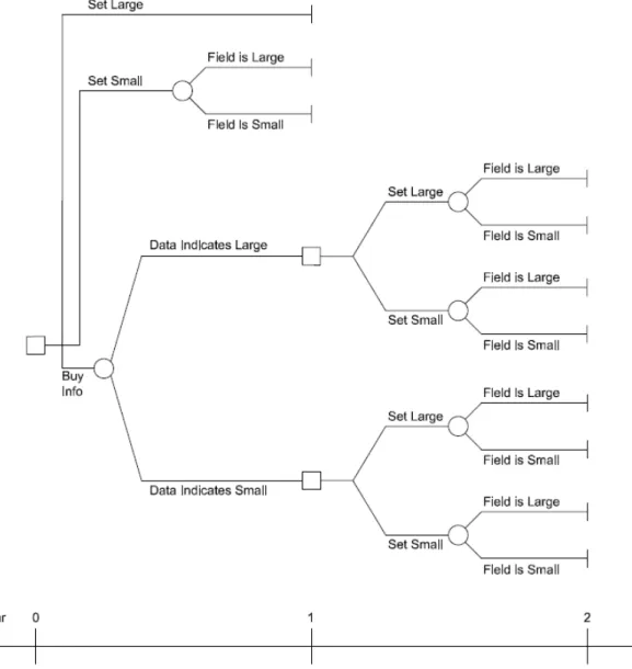
reasoning could be possible, but as it is not, the best decision might still be to develop a large platform, even if the new data indicates the presence of a small amount of oil in the geological structure (e.g. the downside of the potential losses in the case of a large amount of oil could be so disastrous, which would justify the option to implement a LP). The decision tree depicting all these options can be seen in the figure below, where the represented time steps are annual, and the squares reflect decision nodes whereas circles indicate resolution of exogenous uncertainty.
Figure 1 Oilfield Development Decision Tree
Considering all stated values are present values, a particular set of assumptions are developed to help clarify the above decision process. The objective is to determine the option that best minimizes expected costs, having access to the following data:
• construction of a LP has an estimated cost of $90 million2;
• construction of a SP has an estimated cost of $30 million. However, if it is later found that a large amount of oil is in fact the case, the installation of a second platform and all associated costs represent an additional cost of $90 million. Thus, in this later case, the total cost amounts to $120 million;
• drilling a second delineation well and deferring the decision has an estimated cost of $5 million. The team considers that there is a 90% probability that the data collected by this second well will be sufficient to determine the size of the discovery – there is thus, a 10% probability that the collected data will not be sufficient (i.e. not perfect information) to properly determine the size of the discovery.
Before introducing the above values to the developed decision tree, it is necessary to compute the effect of new information on our current estimates. This procedure will be achieved by using Bayes’ Rule (overviewed in Appendix A), which can be seen in the tables below. The first table defines the possible states of nature, and the following three tables determine the effect of the new data in the current estimates.
State of Nature Description
E1 Large quantity of oil
E2 Small quantity of oil
Table 1 Considered States of Nature
State of Nature
Original Probabilities
Conditional Probabilities
Joint Probabilities
Revised Probabilities
E1 0.35 0.90 0.315 0.8289
E2 0.65 0.10 0.065 0.1711
Total 1.00 1.00 0.38 1.00
Table 2 Probabilities in Case New Data Indicates the Presence of a Large Amount of Oil
State of Nature
Original Probabilities
Conditional Probabilities
Joint Probabilities
Revised Probabilities
E1 0.35 0.10 0.035 0.0565
E2 0.65 0.90 0.585 0.9435
Total 1.00 1.00 0.62 1.00
Table 3 Probabilities in Case New Data Indicates the Presence of a Small Amount of Oil
Joint Probabilities
Table 2 result 0.38
Table 3 result 0.62
Total 1.00
Table 4 Joint Probabilities Addition
The calculations developed in the above tables permit the decision tree to be completed, which is shown in the figure below.
Figure 2 Oilfield Development Decision Tree with Computational Results
In order to consider the effect of changing key parameters a sensitivity analysis is developed. The effects of changing the involved cost in the case of setting a SP and later discovering that there is a large quantity of oil in the site, of changing the probability that the acquired additional data will be sufficient to determine the quantity of oil present in the site, of changing the initial probability that the case is a large quantity of oil, and of changing the cost of acquiring additional information are analysed in the Figures 3, 4, 5, and 6.
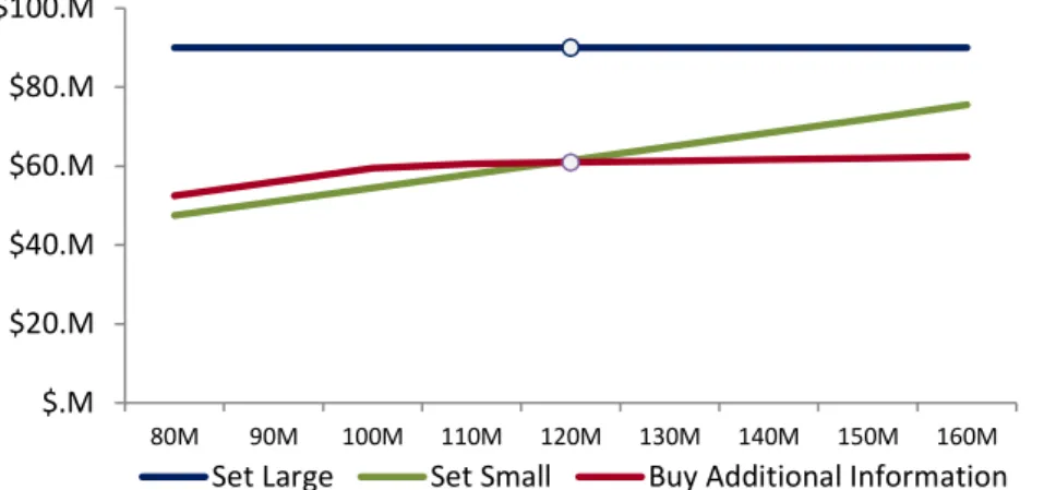
Figure 3 Sensitivity Analysis to Readapting Costs from a Small Platform to a Large Platform
Figure 3 represents the expected required costs to readapt from a SP to a LP. The circled points indicate the current estimated costs, namely $120 million – the ‘Set Small’ and ‘Buy Additional Information’ points are superimposed on one another. It can be seen that setting a small platform is the preferred decision until the level of expense overcomes roughly $118 million, point from which the option to acquire additional information is the one that best minimizes expected costs. From around $1 billion onwards, the “Set Large” option is the path that represents the choice with lowest expenditures.
The graph shown in Figure 4 illustrates the effect of changing the probability that the newly acquired data will be sufficient to determine the amount of oil present in the geological structure. The option to set a SP is the best option to follow until the confidence in the sufficiency of the new data reaches 90%, and from this level onwards the best option is to pursue the purchase of supplementary information.
Figure 4 Sensitivity Analysis to New Data Being Sufficient to Determine Quantity of Oil
$.M $20.M $40.M $60.M $80.M $100.M
80M 90M 100M 110M 120M 130M 140M 150M 160M
Set Large Set Small Buy Additional Information
$.M $30.M $60.M $90.M $120.M
30% 40% 50% 60% 70% 80% 90% 100%
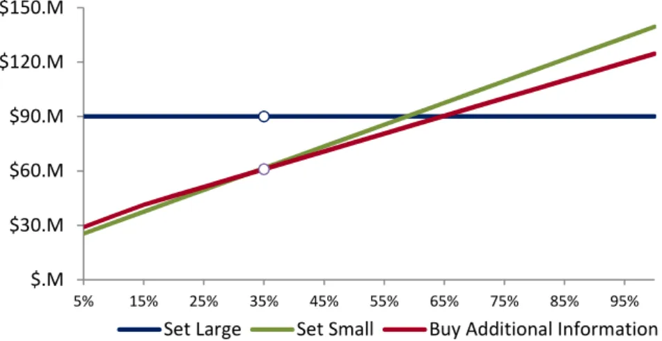
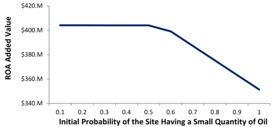
The next analysis is made by altering the value of the initial estimate that the case at hand is a large quantity of oil, which can be seen in Figure 5. ‘Set Small’ is the preferred alternative until about 35%, point from which acquiring additional information becomes the best option. This is so until roughly 65%, where from this point onwards the ‘Set Large’ alternative starts to be the best path to follow.
Figure 5 Sensitivity Analysis to the Initial Probability of Having a Large Quantity of Oil
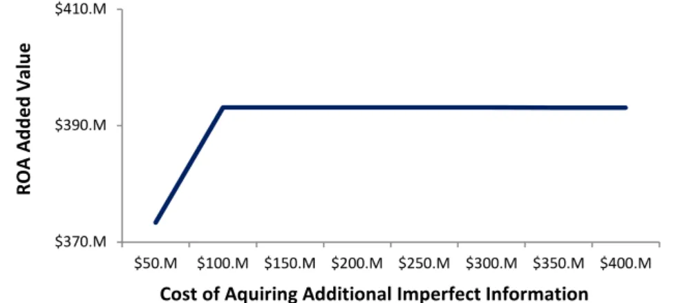
Lastly, in Figure 6, an investigation is developed to changing the price of additional information. ‘Set Large’ and ‘Set Small’ options are unaffected by changing the cost of acquiring new data, as this cost is only applied in the alternative to obtain supplementary information. This study shows that purchasing new data is the best option to follow until the cost of this data reaches around $5.5 million, and from this point onward the option that minimizes expected costs is to set a SP.
Figure 6 Sensitivity Analysis to the Cost of Purchasing Additional Information
$.M $30.M $60.M $90.M $120.M $150.M
5% 15% 25% 35% 45% 55% 65% 75% 85% 95%
Set Large Set Small Buy Additional Information
$.M $30.M $60.M $90.M $120.M
1M 2M 3M 4M 5M 6M 7M 8M 9M 10.00
4. Real Options Analysis
The traditional process in capital budgeting is the use of the Net Present Value (NPV) approach, which uses the DCF technique to value the present values of all future cash flows. These present values minus the initial investment give the NPV of the project, and the rule of the methodology is to accept projects with positive NPV and reject those with negative NPV.
This approach implicitly assumes that once cash flows are established, management will have a passive attitude throughout the project, being irrevocably committed to the set strategy. Thus, NPV fails to consider and properly capture management’s flexibility to adapt and revise later decisions, by not being capable of reviewing the set strategy.
In the real world, and particularly in offshore oil and gas exploration, uncertainty exists, and cash flows will probably vary from management’s expectations. New data will also be identified, which will most likely change the project’s assumptions, and throughout this process the management team will be facing the option to possibly change the defined strategy. Real options analysis valuation methodology brings the required financial flexibility into the valuation of these projects, as the options of deferring, expanding, staging, contracting, learning, or abandoning3 the project throughout its life cycle are taken into account, giving financial and strategic flexibility to the management team.
In this sense, a real option is thus, the right, but not the obligation, to take a certain action at a predetermined cost within or at a specific period of time. Real options methodology is built on their financial counterpart and on the model developed by Fischer Black and Myron Scholes, as modified by Robert Merton. The term “Real Option” was attributed by Stewart Myers in 1977, when it referred that option pricing theory could be used to value investment opportunities in non-financial assets, or “real assets”.
Real options analysis is mainly characterized by the following six basic variables:
• Present value of expected cash flows – this is the present value of the expected cash flows of the investment opportunity under analysis. It corresponds to the stock price on which a conventional option is purchased.
• The exercise price – the required outlay to develop the investment opportunity. Equivalently, it is the defined price for a financial option to be exercised.
• Uncertainty – uncertainty related to the project value. It is a measure of the standard deviation of the present value of expected cash flows. On options theory, it is the stock price volatility.
• Time to expiration of the option – period of time during which, or at which, the investment option can be exercised.
• The risk-free rate of interest – rate of a riskless security with the same maturity as the period of existence of the option.
• Dividends – cash flows incurred during the life cycle of the project. Parallels with dividends paid to stockholders in the option pricing model.
To analyse the behaviour of the above parameters, the effect of an increase in each of the variables can be seen below in Table 5.
Increase in Variable Real Option Effect
Present Value of the Asset Increase
Exercise Price Decreases
Uncertainty Increases
Time to Expiration Increases
Risk-free Increases
Dividends Decreases
Table 5 Effect of a value increase on the variables
When compared to financial options, real options are however a more complex instrument. This is the case for a number of characteristics, being the most fundamental one the fact that real options underlying assets are non-tradable assets, making it harder to estimate some of the above discussed parameters, as the “price” of these assets is not usually observable. Another difference is that financial options are derivative securities (i.e. securities whose price is derived from the prices of other securities), which are bought or written by agents that do not have influence over the investment’s course of action, and no control over the company’s share price. This is opposite to real options, where management has control over the company and its investments, and whose actions directly influence the direction given to the company and its investments.
5. Oil Price Stochastic Process
Black and Scholes option pricing methodology description of how assets price evolve through time is based on the Geometric Brownian Motion (GBM)4 assumption. GBM is referred to in financial theory as a random walk, where price movements are independent from one another, and thus, past information cannot be used to predict future movements5.
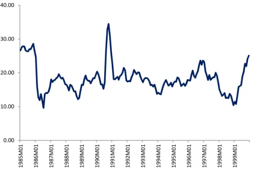
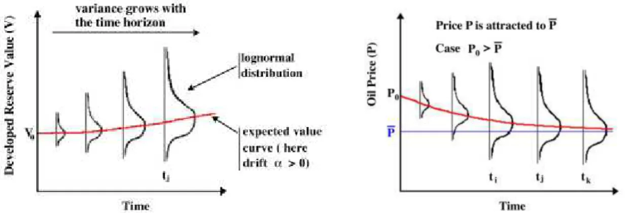
However, energy commodities price behaviour is slightly different from GBM, as for example, if oil prices had a significant increase, producers would increase the supply, which would cause a fall in oil prices. Equally, if oil prices become very low, producers would reduce production, resulting in oil prices to move up to a previous level. This movement is an intrinsic characteristic of energy market prices, and a graphical representation of this behaviour is shown in Figure 7, which shows crude oil price evolution from January 1985 to December 1999. The figure’s price record is an equally weighted crude oil spot price average of Brent, Dubai, and West Texas Intermediate crude oil monthly nominal prices, and presented in US dollars.
Figure 7 Average Crude Oil Price Evolution (Data source: World Bank)
If a pure GBM methodology is used to model oil spot price, unrealistic price levels could be observed, as if because of some abnormal market conditions, a peak price is reached, instead of regressing to a previous mean price level, GBM would continue to move to unrealistic levels.
4 Appendix C describes Geometric Brownian Motion process. 5 Assumption consistent with Efficient Market Hypothesis.
Mean Reversion Model (MRM) describes the type of movement realized by crude oil price, and was first used by Oldrich Vasicek (1977) to model interest-rate dynamics. The method can be thought as an adjustment to random walk, where price movements are not independent from one another, but instead related. The mean reversion process can be described by the following equation6:
Equation 1 Mean Reversion Model (Schwartz, 1997)
where S is the spot price, and α (taken to be strictly positive) is the speed at which the spot price returns to the long term level, ̅ = . σ is the volatility of S, and dz is the Wiener7 process. In this model, if the spot price rises above the long term level, then the drift part of the equation (i.e. α μ − ) will become negative, and the price will tend to move back to the long term level. The random component (i.e. σSdz) will then determine the size and direction of the movement. Similarly, if the spot price is below the long term level, the drift component will be positive, and the price will tend to move up to the long term level.
Although the distribution of futures prices is also lognormal as in GBM, MRM variance increases until a future time, remaining constant after that point is reached. Figure 8 illustrates both processes, where GBM volatility increases with time, and where MRM volatility grows until a certain point in time, after which it remains constant.
Figure 8 GBM and MRM Variance Evolution (Source: Dias, 2004)
An important property of mean reversion is the half-life concept, which is the time taken for the price to move half way back from its current level to its long term level, assuming no more random shocks occur. This is an average time (over a long period of time) that provides a good sensitivity to the “velocity” of the mean reversion process, in alternative to
α, which is a value between 0 and 1 and not so intuitive. Mathematically, half-life is given by the next equation.
6 This formulation is one of several possible equations that capture the same type of market price evolution. 7 Discussed in Appendix C.
Sdz Sdt
S
Equation 2 Half-Life
Oil price movement is thus, more accurately captured by the mean reverting model, ‘more consistent with futures market, with long-term econometric tests and with microeconomic theory’ (Dias, 2004), and as such, MRM will be the employed model to estimate oil price evolution.
5.1. Estimating Mean Reversion Parameters
Unlike GBM models that have the advantage of input parameters being relatively easy to estimate, and where volatility can be considered as the most complicated parameter to evaluate, mean reversion models require the estimation of additional parameters. As referred above, these are the long term level ( ̅ , and the rate (α) at which the spot price reverts to ̅.
Mean reversion parameters can however be robustly estimated through linear regression. As indicated in Shimko (2002), and Clewlow and Strickland (2000), the simple mean reverting process, where µ represents the long run mean, can be rewritten as:
Equation 3 Simple Mean Reverting Process Rewritten
This is just like a regression with dependent variable (Xt+1-Xt) and independent variable Xt
with intercept αµ, and slope -α. If the estimated α is negative (the slope is positive), there is no mean-reversion, and if α is positive (the slope is negative), there is indication that mean reversion is present in the process. Statistical significance of α should then be tested by looking at the parameter t-statistic (p-value can also be a good indicator), and being α statistically significant, error homoscedasticity, normality, and independence tests should also be carried out to test the validity of the hypothesis.
Concluding all statistical tests, the mean reversion speed is estimated by:
Equation 4 Mean Reversion Speed
and, the long run mean by:
Equation 5 Mean Reversion Long Run Mean
Volatility can be estimated using the regression standard error, in which case, as referred by Clewlow and Strickland (2000), it is necessary to note that this standard error is expressed in dollars, and not with no unit expression, like the volatility obtained from logarithmic price
α
) 2 ln( 2 /
1 =
t
1
1 +
+ − t = − t + t
t X X
X αµ α ε
α µ =intercept
slope − =
returns. Thus, the volatility percentage obtained from linear regression will be estimated by the following equation:
Equation 6 Linear Regression Volatility
In the development of the oil price analysis both methods of volatility estimation will be carried out, and after assessment, one of these will be selected for the project development.
µ
6. Approach to Project Resolution
In order to guarantee data confidentiality, the studied project represents a general case hypothesis, where the used figures are typical industry values. The analysis is first developed over a simplified case, which allows for the introduction of the used methodologies, being the full exploration scenario developed at a later stage. In the later complete case, both binomial and trinomial methodologies are considered, which correspond to the GBM and MRM approaches, and a comparison between the obtained results is also realized.
The valuation of the project is addressed by defining two sources of uncertainty, namely, price uncertainty and technological uncertainty. Price uncertainty represents market oil price and its evolution through time, and technological uncertainty in the first stages of the investigation process will constitute the uncertainty of the existence of oil in the surveyed site, and at later stages, if the presence of oil is confirmed, technological uncertainty will characterize the amount of oil that is present in the site.
These uncertainties have different “behaviours” through time, as price uncertainty is known today and becomes more unclear as time evolves, and technological uncertainty reduces through time as more information about the site’s geological structure becomes known. Furthermore, technological uncertainty will not get resolved smoothly over time, as for example in a Brownian motion process, being instead resolved at the moment new information becomes available. Therefore, it is not adequate to produce an estimate for the technological volatility and use it to generate the common binomial or trinomial lattice, which assumes that uncertainty is resolved continuously through time.
It is thus, necessary to construct two separate trees that reflect the resolution of both price and technological uncertainties, in order to correctly develop the ROA valuation. Following the methodology presented in Copland and Antikarov (2003), and their introduction to the Quadranomial Approach, in the case of a binomial lattice four outcomes will be possible at the end of the first period. At this point in time, each uncertainty tree will have either moved up or down, and the value of the project, V0, will be obtained by the combination of these
Figure 9 Quadranomial Possible Outcomes Figure 10 Call Option Value
The quadranomial event lattice has four branches at every node, representing a generalization of the binomial event lattice with two branches at every node, and Figure 10 expresses the valuation of a call option after one period.
As the existence, and possible quantity of oil present in the geological structure is not in any manner influenced by developments of oil price in international markets, technological uncertainty is considered to have a beta of zero. Equation 7 shows that with a = 0, the appropriate discount rate is the risk free rate.
Equation 7 Technological Uncertainty Discount Rate Computation
The independence between the project’s two uncertainties, also has the result that the neutral probabilities of each branch of the quadranomial lattice, to be the product of the risk-neutral probabilities of the same identical branch on the price and technological uncertainties trees. Therefore, for each node, the probabilities will be:
Equation 8 Quadranomial Tree Risk-Neutral Probabilities
where π represents the quadranomial lattice risk-neutral probability, and p the individual uncertainty risk-neutral probability. In addition, it is relevant to note that the assumption of technological uncertainty being independent from market movements, also implies that this uncertainty’s real and risk-neutral probabilities are equal.
The characterization of oil price movement, as refereed above, will be better captured by the mean reverting model. For this purpose, Hull (2009) trinomial tree building procedure8 will be the used methodology to describe oil price evolution through time. By combining this oil price
8
This procedure is discussed in Appendix D.
rf ] rf r [ rf
rtec = +βtec M − =
trinomial tree with the technological uncertainty tree, a Hexanomial tree will be created, and six outcomes will be possible at the end of one period. The hexanomial tree will be resolved in a manner completely identical to the quadranomial tree, but having six branches at every node. Figure 11 demonstrates this process, and as realized for the quadranomial process, the right hand side of the figure also develops the valuation of a call option after one period.
7. Simplified Case
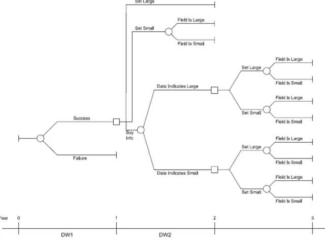
The simplified case is based on the simple stylized example used earlier, motivating the application of ROA. The case develops the scenario of an offshore site where a delineation well (DW1) will be drilled, and in case the test is productive, management faces the decisions discussed in point 3 of this thesis, which are the establishment of a LP, of a SP, or the acquisition of additional imperfect information (DW2). As before, setting a LP can be considered as a “safe” strategy, installing a SP as a “gamble” strategy, and the acquisition of additional imperfect information as an alternative that will defer the decision for one year. This process can be seen below in Figure 12, where the indicated time steps are also annual.
Figure 12 Simple Case Oilfield Development Decision Tree
Appendix E and Appendix F respectively show project technological and price uncertainties data, constituting the data available to the management team at time zero. Price uncertainty appendix also includes all necessary calculations to the construction of a trinomial tree, and the effect of new information to technological uncertainty is exposed in Appendix G.
In year one, if DW1 is unsuccessful, the project is discontinued with no nodes emanating from failure nodes. If DW1 is successful, management will face the discussed alternatives, and will have to analyse the NPV of each mutually exclusive alternative. This is the base case scenario, where without the consideration of ROA management would select the alternative with best NPV.
0 1 2 3 0 1 2 3
PV s B sb(D+) E sb(D+)LO J PV s B sb(D+) E $132,210,536.07 s C sb(D+) F sb(D+)LO K s C sb(D+) F $91,186,975.28 s D sb(D+) G sb(D+)LO L s D sb(D+) G $62,518,791.60
f B sb(D+) H sb(D+)LO M f B sb(D+) H $42,484,822.35
f C sb(D+) I sb(D+)LO N f C sb(D+) I $28,484,635.65
f D sb(D+)LO O f D $18,700,991.42
sb(D+)LO P $11,863,961.57
sb(D+)SO J $126,210,536.07
sb(D+)SO K $85,186,975.28
sb(D+)SO L $56,518,791.60
sb(D+)SO M $36,484,822.35
sb(D+)SO N $22,484,635.65
sb(D+)SO O $12,700,991.42
sb(D+)SO P $5,863,961.57
sb(D-) E sb(D-)LO J sb(D-) E $132,210,536.07 sb(D-) F sb(D-)LO K sb(D-) F $91,186,975.28 sb(D-) G sb(D-)LO L sb(D-) G $62,518,791.60 sb(D-) H sb(D-)LO M sb(D-) H $42,484,822.35 sb(D-) I sb(D-)LO N sb(D-) I $28,484,635.65
sb(D-)LO O $18,700,991.42
sSO E sb(D-)LO P $87,044,264.46 $11,863,961.57 sSO F sb(D-)SO J $57,816,706.90 $126,210,536.07 sSO G sb(D-)SO K $37,391,834.65 $85,186,975.28 sSO H sb(D-)SO L $23,118,476.17 $56,518,791.60 sSO I sb(D-)SO M $13,143,933.38 $36,484,822.35
sS§ E sb(D-)SO N $46,022,132.23 $22,484,635.65
sS§ F sb(D-)SO O $31,408,353.45 $12,700,991.42
sS§ G sb(D-)SO P $21,195,917.33 $5,863,961.57
sS§ H $14,059,238.09
sS§ I sb(D+)L§ J $9,071,966.69 $66,105,268.04
sb(D+)L§ K $45,593,487.64
sL E sb(D+)L§ L $62,804,878.51 $31,259,395.80 sL F sb(D+)L§ M $43,076,277.16 $21,242,411.18 sL G sb(D+)L§ N $29,289,488.39 $14,242,317.83 sL H sb(D+)L§ O $19,654,971.42 $9,350,495.71 sL I sb(D+)L§ P $12,922,155.03 $5,931,980.78
sb(D+)S§ J $65,605,268.04
sb(D+)S§ K $45,093,487.64
sb(D+)S§ L $30,759,395.80
sb(D+)S§ M $20,742,411.18
sb(D+)S§ N $13,742,317.83
sb(D+)S§ O $8,850,495.71
sb(D+)S§ P $5,431,980.78
sb(D-)L§ J $66,105,268.04
sb(D-)L§ K $45,593,487.64
sb(D-)L§ L $31,259,395.80
sb(D-)L§ M $21,242,411.18
sb(D-)L§ N $14,242,317.83
sb(D-)L§ O $9,350,495.71
sb(D-)L§ P $5,931,980.78
sb(D-)S§ J $65,605,268.04 sb(D-)S§ K $45,093,487.64 sb(D-)S§ L $30,759,395.80 sb(D-)S§ M $20,742,411.18 sb(D-)S§ N $13,742,317.83
sb(D-)S§ O $8,850,495.71
sb(D-)S§ P $5,431,980.78
Figure 13 Simple Case Hexanomial Event Tree
In the figure above, the code on the left hand side of each node describes technological uncertainty path, and the letters at the node’s right hand side indicate the possible price
s – success f – failure b – buy info S – set small L – set Large O – result is large § – result is Small (D+) – data says it is large (D–) – data says it is small
Technological uncertainty legend:
Colours Legend (Y2 and Y3): Buy info; Result is (D+)
Data indicates (D+); Set LP Data indicates (D+); Set SP Buy info; Result is (D-) Data indicates (D-); Set LP Data indicates (D-); Set SP Set LP at Y3
Set SP at Y3; It is large Set SP at Y3; It is small Abandon
levels at that year. Blue and brown shaded cells represent the alternative of acquiring additional information, where the blue cells characterize the case that the new data indicates a large quantity of oil, and brown cells portray the case where a small quantity of oil is determined by the obtained information. Year three blue sb(D+)L cells embody the path where management decides to set a LP, with O representing the case that the site has in fact a large quantity of oil, and § expressing the situation that the site has a small quantity of oil. Similarly, blue sb(D+)S symbolize the case where management establishes a SP.
Identically, third year sb(D-)L brown cells indicate the path where management sets a LP, with O being the case of a large quantity of oil, § the case of a small quantity, and sb(D-)S depict the alternative route where management sets a SP. With a similar reasoning, year two green cells depict the option where management sets a SP, and violet shaded cells represent the alternative of setting a LP, being the reading of all these possibilities easily followed by the figure’s legend.
Dependent on the followed option, at the end of the second or third year oil quantity uncertainty will have been resolved, and a DCF model can be developed for each possible result at each level of oil price. The values on the cells are the obtained results, and the cash flow models for each of the end nodes can be found in the referred appendix.
The first alternative NPV to be computed is the option to acquire additional information, where the tree’s end nodes NPVs are worked backward until year zero, being the project Present Value (PV) obtained. In order to develop this process it is necessary to have each node’s combined probabilities (i.e. π), which are showed in Appendix I. The risk-neutral probabilities are then used to calculate the value at each node, and for example node sb(D+) E, is the maximum value between the choice of either setting a large or a small platform. Computationally, this is the maximum between (monetary values are expressed in millions):
and:
In the above, the value for the case of setting a LP (i.e. top equation) is obtained by multiplying end nodes sb(D+)LO J, sb(D+)LO K, and sb(D+)LO L respectively by the LO*(E)pu, LO*(E)pm, and LO*(E)pd risk–neutral probabilities, which are indicated in the Buy info, data indicated large quantity, do large platform – To Point E section of the simplified case trinomial tree nodes probabilities table. The one year risk-free discounted value obtained by this multiplication, has to be reduced by the year two cost of installing a large platform multiplied by the probability that a large quantity of oil is the case. The value obtained by these computations is added to the value that although the new information indicated a large quantity of oil to be present in the site, and a LP was set, the actual case is that a small quantity is present in the geological structure.
Therefore, in an identical procedure, this last value is obtained by multiplying end nodes sb(D+)L§ J, sb(D+)L§ K, and sb(D+)L§ L respectively by the L§*(E)pu, L§*(E)pm, and L§*(E)pd risk–neutral probabilities, whose result is discounted to year two at the risk-free rate. At year two, the investment of installing a large platform multiplied by the probability that a small quantity of oil is the case is also reduced from the discounted value. The addition of these two results will constitute the value of setting a LP when the new information indicates a large quantity of oil.
It is necessary to refer that at the end of the computation of both possible outcomes, the reduction of year two cost of setting up a LP was multiplied by each outcome probability. The result would be the same, if the platform installation full cost was reduced at the end of the equation, without multiplying it by any probability. Although this is the case in this possible path, as it is showed next, this will not be the case in other possibilities, and thus, the computation was constructed in this manner in order to maintain calculations uniformity.
The above result is for the option of setting a LP when the new data indicates a large quantity of oil, but as referred, at this point in time (i.e. year two) management can also decide to install a SP (the second equation), whose computation is constructed in a similar manner to the calculations described above. Thus, this path result is achieved by multiplying end nodes sb(D+)SO J, sb(D+)SO K, and sb(D+)SO L respectively by the SO*(E)pu, SO*(E)pm, and SO*(E)pd risk–neutral probabilities, which are indicated in the Buy info, data indicated large quantity, do small platform – To Point E section of the same simplified case probabilities table. The one year risk-free discounted value obtained by this multiplication, is reduced by the year two total infrastructures cost multiplied by the probability that a large quantity of oil is the case. This infrastructures total cost includes the penalty costs of installing a SP, and later finding that the site has a large quantity of oil. Hence, the infrastructures total cost is composed by the cost of installing a small platform, plus the cost of setting a second platform and readapting the extraction system.