A study on the accuracy and precision of external mass
transfer and diffusion coefficients jointly estimated
from pseudo-experimental simulated data
I.C.A. Azevedo1,a, F.A.R. Oliveirab,*, M.C. Drumonda
a
Escola Superior de Biotecnologia, Universidade CatoÂlica Portuguesa, Rua Dr. AntoÂnio Bernardino de Almeida, 4200 Porto, Portugal
b
Instituto Inter-UniversitaÂrio de Macau, PalaÂcio da Penha, Macau
Abstract
Optimal experimental designs for maximum precision in the estimation of diffusivities (D) and mass transfer coefficients (Kc) for solute transport from/to a solid immersed in a fluid were determined. Diffusion in the solid was considered to take
place according to Fick's second law. It was found that the optimal design was dependent on the Biot number. In the range of Biot numbers tested (0.1±200), the first sampling time corresponded to values of fractional loss/uptake between 0.10 and 0.32, and the second sampling time corresponded to values of fractional loss/uptake between 0.67 and 0.82. Pseudo-experimental data were simulated by applying randomly generated sets of errors, taken from a normal distribution with 5% standard deviation, to data calculated using given values of the model parameters. Both optimal and heuristic designs (for which the sampling times corresponded to values of fractional loss/uptake from 0.30 to 0.95) were analyzed. The accuracy and precision of the estimates obtained by non-linear regression were compared. It was confirmed that optimal designs yield best results in terms of precision, although it was concluded that the joint estimation of D and Kcshould, in general, be avoided. For
intermediate values of the Biot number, reasonably precise and accurate estimates can however be obtained if the experimental error is small.#1998 IMACS/Elsevier Science B.V.
Keywords: Heuristic experimental design; Mass transfer parameters; Optimal experimental design; Parameter estimation
1. Introduction
When modeling mass transfer of solutes from/to solids immersed in fluids, most authors assume that the resistance of the fluid to mass transfer is negligible [1±4]. For this assumption to be valid, the experiments are often carried out with stirring of the fluid. However, in some cases, the stirring may not be enough to completely destroy the external resistance. Nicolas and Duprat [5] reported that the
ÐÐÐÐ
* Corresponding author. Tel.: +853-968793/4; fax: +853-968813.
1
Tel.: +351-2-5580044; fax: +351-2-590351
diffusion coefficient (D) of potassium nitrate in agarose depended on the degree of stirring and concluded that with low stirring there was a boundary layer that affected the mass transfer rate. However, they did not measure external mass transfer coefficients. Potts et al. [6] studied the mass transfer of several solutes between cucumbers and brine solutions. They assumed that the major resistance to mass transfer was in a stagnant layer surrounding the cucumber and determined only the external mass transfer coefficient (Kc).
Only a few studies were reported in which both internal and external resistances are taken into
account. Azevedo and Oliveira [7] estimated DandKcin a conventional way: first, Dwas estimated
from experimental data obtained under high stirring, so that the external resistance was confirmed to be negligible; then, experiments were carried out without stirring andKcwas estimated using the value of
D obtained from the first set of experiments. One important conclusion from this work was that the
model which neglects the external resistance also fits well the data from the static experiments, although leading to inaccurate values ofD. Azevedo and Oliveira [8] have also theoretically analyzed the influence of assuming negligible external resistance to mass transfer on the accuracy and precision of the estimated value ofD. It was concluded that for very large values of the Biot number (Bi) this assumption is valid, whereas for intermediate values of the Biot number significant errors arise, despite an apparent good fit between the data and the model.
Other studies apply multi-parametric regression to determine simultaneouslyDandKcfrom a single
experiment (e.g. [9]). Multiparametric analyses may however be unreliable and the use of an adequate experimental design is very important in order to accurately and precisely estimate the kinetic parameters. In fact, even a very careful analysis of experimental data is unable to recover information that is not present in that data [10]. In general, if the mathematical model is known, optimal experimental designs are very useful to estimate parameters with increased precision. Box and Lucas [11] proposed an optimum design based on determining the sampling conditions that lead to a minimum confidence region for the case where the number of experimental points is equal to the
number of parameters. This design, also known as D-optimal design, was applied to different models,
such as a first order kinetics [11], diffusional processes [12] and to the Bigelow model [13]. It was further shown that for a number of points larger than the number of parameters, this design often corresponds tor replicates of the optimal psampling times (rN/p) [14].
However, alternative experimental plans based on common sense are often used instead of optimal designs, because they are much more straightforward and they do not require a full knowledge of the model parameters. The most common heuristic plans used are those corresponding to taking samples at equally spaced values of the fractional loss/uptake of solute, equally spaced values of time, or equally spaced values of the logarithm of time.
The objectives of this work were (i) to define optimal experimental designs for maximum precision in the joint estimation of diffusivities and mass transfer coefficients, (ii) to assess if the parameters estimated with these designs are both accurate and precise, and (iii) to compare the accuracy and precision of these estimates with those obtained by heuristic designs.
2. Methods
volume of solution, is [15,16]
Mt
M1
1ÿ X
1
n1
2Bi2
2
n 2nBi
2Biexp ÿ 2
nDt=L
2
" #3
(1)
whereMtis the total amount of solute uptake/loss at timet,M1the total amount of solute uptake/loss at
equilibrium,Lthe half-thickness of the cube,Dthe diffusion coefficient, Bi the Biot number (BiLKc/
(KpD)),Kcthe mass transfer coefficient,Kp the partition coefficient, and nthe roots of the equation
tanBi.
For a specific set of the model parameters, this equation allows the calculation of values of Mt/M1
for a given time. The values of time for this calculation were chosen both according to optimal and heuristic designs. A wide range of Biot numbers were considered, from 0.1 to 200. Early studies have shown that the values ofD,Kc,KpandL, on their own, do not influence the accuracy and precision of
the diffusivities and mass transfer coefficients estimated. For calculation purposes, the following values
were then used, without loss of generality: D110ÿ9m2sÿ1, Kp1, L0.01 m. The Biot
numbers were then calculated assuming different values of Kc.
2.1. Optimal design
The D-optimal design concept was applied, considering a number of sampling times equal to the
number of parameters and five replicates of each sampling time. Minimization of the error region of the parameters corresponds to maximization of the determinant of the derivatives of the model function (f) in order to the parameters [11,14]. For the case of two parameters, the determinant is given by
jNj
PN i1
@f
@p1
2
i
PN i1
@f
@p1
@f
@p2
i
PN i1
@f
@p1
@f
@p2
i
PN i1
@f
@p2
2 i (2)
where Nis the number of points, andp1andp2are the parameters.
For each Biot number, the two sampling times (and the corresponding values of Mt/M1) that
maximized the absolute value of the determinant in Eq. (2) were determined; the functionfcorresponds to Eq. (1) andDandKcare the parameters of interest. The Simplex method for minimization was used;
the objective function was the reciprocal of the determinant. For these calculations, a subroutine was written in FORTRAN 77.
2.2. Heuristic design
In this work, a heuristic design based on equally spaced values of Mt/M1 was used. Ten sampling
times were considered, for values of Mt/M1 ranging from 0.3 to 0.95: for values of Mt/M1 smaller
than 0.7, the time interval was chosen so that the increase of Mt/M1 from one sampling point to the
next was 0.1, whereas for larger values of Mt/M1 this interval was 0.05.
The efficiency of the heuristic design (") was calculated by
" jNj
HD
jNjOD
" #1p
where p is the number of parameters (in this case, p2) and the superscripts HD and OD refer to heuristic design and optimal design, respectively.
2.3. Pseudo-experimental data generation
Pseudo-experimental data were calculated by applying to the values ofMt/M1a set of random errors
taken from a population with normal distribution with zero mean and 5% standard deviation. Twelve different sets of random errors were tested. The average and standard deviation of each set of errors are shown in Fig. 1.
For the optimal design, five replicates of eachMt/M1 were considered, giving a total of 10 points,
the same number of points used for the heuristic design. The pseudo-experimental data were generated in the same manner for both designs, using the same sets of errors.
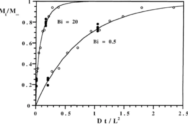
Fig. 2 shows typical simulated curves and pseudo-experimental data, for both optimal and heuristic designs. The pseudo-experimental data shown in this figure were generated using a set of errors with
ÿ0.00114 average and 2.8839% standard deviation (set min Fig. 1).
Fig. 1. Standard deviation and average of the 12 sets of errors attributed to the values ofMt/M1obtained by simulation.
2.4. Estimation of parameters
The parameters D and Kc were estimated by non-linear regression using the Simplex method to
minimize the residual (Res) between pseudo-experimental and theoretical data. The residual was calculated by
ResX
N
i1
Mt
M1
p:exp:
ÿ Mt M1
theo:
" #2
(4)
A subroutine was also written in FORTRAN 77for these calculations. A total of 720 runs were done.
The precision of each estimated parameter was calculated by a standardized half-width (SHW), defined as half of the confidence interval, at a 95% level, divided by the estimated value of the parameter. The accuracy was expressed by the absolute value of the fractional error of the estimated parameter relative to its `true' value.
Joint confidence regions forDandKcwere calculated at a 90% confidence level, as described by Box
et al. [17]
Res90% Resmin 1
p
NÿpF0:10 p;Nÿp
(5)
where Resminis the minimum value of the residual defined by Eq. (4); Res90%is the residual for the
90% joint confidence region; andF0.10is theFvalue at a 90% confidence level.
3. Results and discussion
3.1. Optimal and heuristic designs
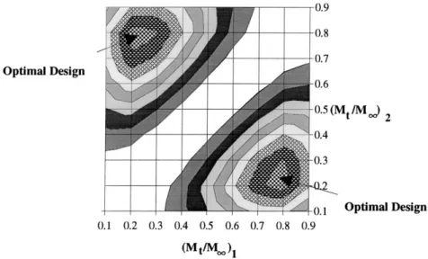
Fig. 3 shows the effect ofMt/M1(and, thus, the effect of the corresponding sampling times) on the
value of the determinant, for Bi20. Similar results were obtained in the whole range of Biot numbers
tested, although the values of Mt/M1 that maximize the determinant were dependent on the Biot
number, as shown in Fig. 4. These values ranged from 0.10 to 0.32 for the first sampling time, and from 0.67 to 0.82 for the second sampling time. Additional calculations have shown that as the Biot number tends to zero, one of the values of Mt/M1 tends to zero and the other to 0.632; this is the result
expected for the case of negligible internal resistance to mass transfer (Mt/M11ÿ1/e [11]). On the
other hand, for very large Biot numbers, one of the values of Mt/M1 tends to zero and the other to
0.704; additional calculations have shown that this is the result obtained when the model for negligible external resistance to mass transfer is used.
3.2. Estimation of parameters
The results shown in Table 1 and Fig. 6 were obtained using pseudo-experimental data generated by
applying a set of errors with ÿ0.00114 average and 2.8839% standard deviation (set m in Fig. 1).
Table 1 shows the results obtained in terms of precision and accuracy of the estimated parameters. For
small values of the Biot number, the joint estimation of D and Kc should be avoided, as even the
application of optimal designs is unable to generate accurate and precise estimates (it should be noted that the higher the values shown in Table 1, the worse the accuracy or precision of the estimated parameters). When estimating the parametersDandKcfor very small Biot numbers, it was noticed that
the correlation coefficients () obtained for both optimal and heuristic designs were very large
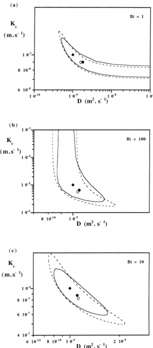
(|| > 0.96 for Bi < 2). Thus, the estimated values of the parameters are not very reliable [18]. This is confirmed by the size and shape of the joint confidence regions shown in Fig. 6(a), which were
Fig. 3. Effect of the values of (Mt/M1)1 and (Mt/M1)2 on the value of the determinant, for Bi20. (Optimal design
corresponds to (Mt/M1)10.23 and (Mt/M1)20.79 or (Mt/M1)10.79 and (Mt/M1)20.23).
obtained for Bi1. It can also be seen that the joint confidence regions for the optimal and heuristic
designs are very similar. The shape of these curves for very large values of D can be explained as
follows: when the diffusivity is very large, the internal resistance to mass transfer is negligible, meaning that the process is controlled by the external resistance; therefore, an increase inDdoes not change the estimated value of Kc.
For Bi3.5, the higher the Biot number the better the precision and the accuracy of the estimated
value of D; the opposite happens in terms of Kc, with accuracy and precision decreasing with the
increase of the Biot number (Table 1). These results were observed both for heuristic and optimal experimental designs; as expected, regarding precision, the optimal design leads to more precise estimates ofDandKc. Curiously it was found that, although the accuracy ofKcis better for the optimal
design, the opposite happens in terms of D. The latter differences, while marginal, show that optimal designs aiming at maximum precision do not necessarily give the best results in terms of accuracy.
For very large values of the Biot number, the estimation ofDis feasible whereas the estimation ofKc
leads to inaccurate values with large confidence intervals (Table 1). This conclusion is also confirmed by an analysis of Fig. 6(b), which shows the joint confidence regions for Bi100. As was verified in Fig. 6(a), the shape of the confidence regions for the optimal and heuristic designs are also very similar. For very large values ofKc, the external resistance to mass transfer is negligible, so that an increase in
Kcdoes not change the estimated value of D.
Fig. 6(c) shows the joint confidence regions for an intermediate value of the Biot number (Bi10). As was verified in Fig. 6(a) and (b), the shape of the joint confidence regions for the optimal and heuristic designs are similar. Because optimal designs lead to maximum precision, the joint confidence region for the optimal design is smaller than that for the heuristic design. This is clearly seen in
Fig. 6(c). One important conclusion from Fig. 6(c) is that, opposite to the cases for Bi1 and
Bi100, the joint estimation of D and Kc for Bi10 might be considered feasible, although the
confidence regions are still large.
As mentioned before, the results shown in Table 1 and Fig. 6 were obtained using a particular set of errors, but all sets of errors shown in Fig. 1 were tested. It was verified that the accuracy and precision of the estimated values ofDandKcdepend on the particular set of errors used to generate the
pseudo-experimental data but the trends observed with the results shown in Table 1 were also observed with the results obtained for all the other sets of errors.
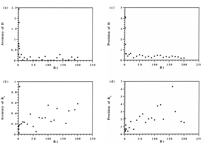
Under real experimental conditions, one expects that the average and the standard deviation of the errors may change from one experiment to another. To analyze the effect of these changes, a different set of errors (randomly chosen) was considered for each Biot number. This study focused only on the optimal design. The results are shown in Fig. 7 (It should be noted that the higher the value in the vertical axis, the worse the accuracy or precision of the estimated parameter). Fig. 7(a) and (c) clearly show that the higher the Biot number, the better the accuracy and the precision of the estimated value of
D. This is in total agreement with the conclusions withdrawn from Table 1. The results shown in
Table 1
Accuracy and precision ofDandKcfor optimal and heuristic designs (considering the set of errorsmwithÿ0.00114 average
and 2.8839% standard deviation)
Biot number Optimal design Heuristic design
Accuracya Precisionb Accuracya Precisionb
D Kc D Kc D Kc D Kc
0.1 0.0730 0.00700 37.7 1.14 0.0630 0.0131 102 3.07
0.25 0.0670 0.00 8.65 0.612 0.0520 0.0152 17.2 1.25
0.5 2.13 0.0888 21.8 0.991 0.751 0.0710 13.5 1.10
0.75 1.35 0.105 6.99 0.589 0.710 0.0924 6.64 0.781
1 0.800 0.101 3.08 0.424 0.598 0.103 3.89 0.619
1.5 0.472 0.101 1.49 0.343 0.495 0.123 2.14 0.497
2 0.330 0.0970 1.02 0.322 0.400 0.130 1.46 0.449
3.5 0.204 0.103 0.612 0.321 0.260 0.143 0.834 0.426
5 0.156 0.107 0.479 0.338 0.205 0.156 0.646 0.445
10 0.107 0.126 0.336 0.406 0.124 0.179 0.446 0.552
15 0.0910 0.147 0.289 0.471 0.0960 0.202 0.385 0.663
20 0.0830 0.165 0.264 0.532 0.0810 0.220 0.354 0.774
30 0.0730 0.193 0.237 0.644 0.0670 0.262 0.324 0.974
40 0.0690 0.222 0.223 0.743 0.0600 0.297 0.309 1.16
50 0.0660 0.247 0.214 0.835 0.0560 0.330 0.300 1.32
60 0.0650 0.278 0.208 0.912 0.0510 0.354 0.294 1.49
70 0.0620 0.296 0.203 0.994 0.0490 0.383 0.290 1.62
80 0.0620 0.318 0.199 1.06 0.0460 0.397 0.286 1.78
90 0.0580 0.328 0.196 1.14 0.0470 0.433 0.284 1.86
100 0.0590 0.350 0.194 1.20 0.0440 0.440 0.282 2.02
110 0.0560 0.361 0.192 1.27 0.0450 0.470 0.281 2.09
120 0.0600 0.386 0.190 1.32 0.0410 0.480 0.279 2.22
130 0.0580 0.396 0.189 1.38 0.0420 0.503 0.278 2.29
140 0.0570 0.408 0.187 1.44 0.0410 0.518 0.277 2.38
150 0.0560 0.424 0.186 1.49 0.0420 0.534 0.277 2.45
160 0.0550 0.436 0.185 1.54 0.0410 0.542 0.276 2.56
170 0.0550 0.449 0.185 1.58 0.0410 0.559 0.275 2.61
180 0.0550 0.457 0.184 1.63 0.0400 0.571 0.274 2.68
190 0.0560 0.468 0.183 1.68 0.0390 0.578 0.274 2.78
200 0.0540 0.477 0.182 1.72 0.0380 0.591 0.274 2.83
a
Accuracy was defined by the absolute value of the fractional error of the estimated parameter relative to its `true' value.
b
Fig. 7(b) and (d), regarding the accuracy and precision of Kc, are more scattered than the results
regarding the accuracy and precision of D, indicating a higher effect of the experimental error in Kc
than inD. It should be mentioned that the results obtained for three values of the Biot number (140, 150
Fig. 6. 90% joint confidence regions for the estimates ofDandKc(considering the set of errorsm), calculated by the heuristic
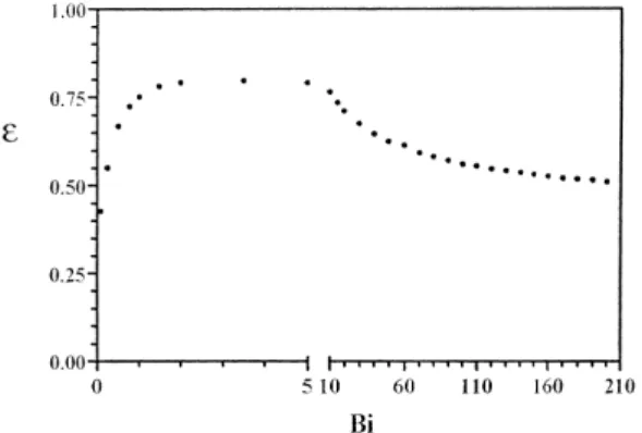
and 180) are not shown in these figures because they would be out of scale. The results shown in Table 1 indicate that the precision ofKcis maximum for Bi around 3.5. (slightly different values were
observed for the other sets of errors tested, but within the same range). However, due to the scatter of the results, the existence of a maximum precision ofKcin the range of small Biot numbers cannot be
clearly inferred from Fig. 7(d). Anyway, it should be reminded that the results obtained in this range of Biot numbers are not very reliable because of the high correlation coefficients. For higher Biot
numbers, Fig. 7(d) shows that the precision ofKcbecomes worse as the Biot number increases, which
is in agreement with the conclusions taken from Table 1. Regarding the accuracy of Kc, the results
shown in Fig. 7(b) are in agreement with those shown in Table 1, that is, the higher the Biot number the worse the accuracy of Kc.
At this point it should be stressed that any set of experiments aimed at determiningDandKcmust be
carefully carried out. In fact, it is not possible to obtain accurate and precise estimates of these parameters if the experimental values are not reasonably accurate and precise themselves. Considering only the results obtained using the sets of errors with standard deviations5%, the following was verified: if a standardized half-width (SHW) of 1 is considered acceptable, then the parameters can in general be estimated for Biot numbers ranging from3.5 to20; if a SHW of 0.5 is considered acceptable, then the
Fig. 7. Accuracy and precision ofDandKc, for optimal design, using a different set of errors (randomly chosen) for each Biot
range of Biot numbers is smaller (5 to15); if only a SHWof 0.1 is considered acceptable, then there is no range of Biot numbers for which the joint estimation ofDandKcis possible.
As suggested from the results shown in Table 1 and Fig. 6, as well as from the observations stated in the previous paragraph, the joint estimation ofDandKcmight only be feasible for intermediate values
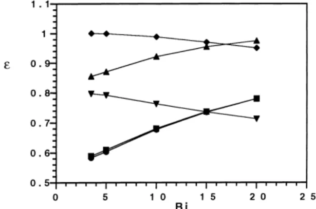
of the Biot number. The results also clearly suggest that it is better to plan the experiments using the optimal design. However, this would only be possible if the Biot number was known `a priori', which is generally not the case. With this in mind, additional calculations were done aimed at comparing the efficiency of the heuristic design with the efficiency of four different designs, each considering five
replicates of two different values of Mt/M1. In three of these designs, the values of Mt/M1
corresponded to values earlier determined for the optimal design for Bi0.1 (Design 1), Bi200
(Design 2) and Bi3.5 (Design 3). The values ofMt/M1used in Design 4 corresponded to the average
values for all the Biot numbers tested in this work. Fig. 8 compares the efficiency of these four designs with that of the heuristic design, in the range of Biot numbers where estimation ofDandKcmight be
feasible. It can be seen that Designs 3 and 4 have higher efficiencies than the heuristic design. In particular, the use of Design 3 is recommended because its efficiency is always very close to unity. As shown in the legend of Fig. 8, the values ofMt/M1for this design are 0.317 and 0.815. These values of
Mt/M1are particularly attractive because they are neither close to the begining of the experiment nor
close to equilibrium.
4. Conclusions
Overall, it can be concluded that the joint estimation ofDandKcshould, in general, be avoided. For
intermediate values of the Biot number, reasonably precise and accurate estimates can only be obtained if the experimental error is small.
Acknowledgements
The authors acknowledge the support received from the European Commission within the framework of the STD3 project TS3*-CT94-0333.
References
[1] A.P. Andersson, R.E. OÈ ste, Diffusivity data of an artificial food system, J. Food Eng. 23 (1994) 631±639.
[2] A.S. Bassi, S. Rohani, D.G. Macdonald, Measurement of effective diffusivities of lactose and lactic acid in 3% agarose gel membrane, Biotechnol. Bioeng. 30 (1987) 794±797.
[3] B.J.M. Hannoun, G. Stephanopoulos, Diffusion coefficients of glucose and ethanol in cell-free and cell occupied calcium alginate membranes, Biotechnol. Bioeng. 28 (1986) 829±835.
[4] L.A. Moreira, F.A.R. Oliveira, T.R. Silva, Prediction of pH change in processed acidified turnips, J. Food Sci. 57 (1992) 928±931.
[5] M. Nicolas, F. Duprat, Determination de la diffusivite du nitrate de potassium en milieu modele PreÂliminaries a l'eÂtude de leÂxtraction des composeÂs solubles lors du blanchiment, Sciences des Aliments 3 (1983) 615±628.
[6] E.A. Potts, H.P. Fleming, R.F. McFeeters, D.E. Guinnup, Equilibration of solutes in non-fermenting, brined pickling cucumbers, J. Food Sci. 51 (1986) 434±439.
[7] I.C.A. Azevedo, F.A.R. Oliveira, A model food system for mass transfer in the acidification of cut root vegetables, Int. J. Food Sci. Technol. 30 (1995) 473±483.
[8] I.C.A. Azevedo, F.A.R. Oliveira, On the estimation of diffusion coefficients under conditions of uncertainty in relation to the existence of significant external resistance to mass transfer, in: Institute of Food Technologists Annual Meeting, 14± 18 June 1996, New Orleans, LA, USA.
[9] C. Engels, M. Hendrickx, S. De Samblanx, I. De Gryze, P. Tobback, Modelling water diffusion during long-grain rice soaking, J. Food Eng. 5 (1986) 55±73.
[10] D.M. Bates, D.G. Watts, Nonlinear regression analysis and its applications, Wiley, New York, 1988, pp. 121±127. [11] G.E.P. Box, H.L. Lucas, Design of experiments in non-linear situations, Biometrica 46 (1959) 77±90.
[12] F.A.R. Oliveira, T.R. Silva, J.C. Oliveira, Optimal experimental design for estimation of mass diffusion parameters using non-isothermal conditions, Proc. of the 1st Int. Symp. on Mathematical Modelling and Simulation in Agriculture and Bio-Industries of IMACS/IFAC, 9±12 May 1995, Brussels, Belgium .
[13] L.M. Cunha, F.A.R. Oliveira, T.R.S. BrandaÄo, J.C. Oliveira, Optimal experimental design for estimating the kinetic parameters of the Bigelow model, J. Food Eng. (1997), in press.
[14] A.C. Aktinson, W.G. Hunter, The design of experiments for parameters estimation, Technometrics 10 (1968) 271±289. [15] J. Crank, Mathematics of Diffusion, 2nd ed., Oxford University Press, London, 1979, pp. 60±61.
[16] A.H. Newman, Ind. Eng. Chem. 28 (1936) 545.
[17] G.E.P. Box, W.G. Hunter, J.S. Hunter, Statistics for experimenters: An introduction to design, data analysis and model building, Wiley, New York, 1987, pp. 484±487.