Mladen LATkOVIĆ, MSc.* Preliminary communication**
Raiffeisen Mandatory Pension Fund UDC 369.914
Management Company, Zagreb JEL H0
Ivana LIkER*
Raiffeisen Mandatory Pension Fund Management Company, Zagreb
Abstract
In this article we analyze the effect of parameters in the standard model for calcula-tion of accumulated savings in a defined contribucalcula-tion pension system. Three parameters affect accumulated savings in the standard model: saving duration, return of the pension fund and the growth in employee gross wage. By using a linear approximation we calcu-lated marginal contributions for small changes in the parameters of the standard model and analyzed their relations for a set of referent parameters which are most suitable for the 2nd pillar pension system in Croatia. It is shown that the return of a pension fund has
a major influence on accumulated savings, while the influence of the growth in employee gross wage is slightly smaller. Also, we calculated the influence of raising the contributi-on rate in the 2nd pillar on the accumulated savings in a simple scenario in which that rate
is raised by equal amounts over the whole of a saving period. These results allow easier planning of pension insurance in the defined contribution system at a general level as well as at an individual level.
Key words: defined contribution system, pension funds, parametric model, sensitivi-ty analysis.
* Authors thanks two anonymus referees for valuable comments and suggestions. ** Received: June 1, 2009
1 Introduction
Collective schemes of investments in a form of pension funds are usually employed in pension insurance systems based on individual capitalized savings. At the moment of retirement, the accumulated savings are transferred to the pension insurance company re-sponsible for annuities payment. The standard model for calculation of accumulated sav-ings (Šorić, 2000) is based on the premises that the contributions are paid to a pension fund at equal time periods, that the contributions have a constant growth rate, and the long-term average annualized rate of return of a pension fund can be used as a proxy for ex-pected profit on invested funds. Such a simplified model enables easier design of man-datory and defined contribution individual pension schemes, which are today widely known as the 2nd pillar pension system.
Due to the numerous simplifications of the standard model and its use of just a few parameters, it is useful to analyze in detail the characteristics of a defined contribution system. The chosen parameters of the standard model have a major influence on person-al accumulated savings. Although the detailed characteristics of the model parameters are very important, we will mention only their basis characteristics in order to determine the model validity range and the referent values of the parameters. The main goal of this ar-ticle is the construction of sensitivity factors that provide a way to analyze the influence of standard model parameters on accumulated savings. These sensitivity factors are used to determine changes in accumulated savings with small changes in parameter values and to analyze relations between standard model parameters for some reference values. We should stress that above mentioned approach to the calculation of accumulated savings can be employed only with respect to an average member of a pension fund, and is hard to reconcile with any individual member of a pension fund. However, since all pension schemes are long-term, most parameter deviations from those of an average member are usually reduced to an acceptable level.
The expected rate of income growth is the parameter that is most individual as it de-pends on the growth of personal income during the employment period. This parameter has two major contributions: one is income growth due to GDP growth and the other is income growth due to personal promotions during the employment period. In order to de-termine the income growth we shall use statistical data for gross wages across all persons in paid employment as a collective indicator of average earnings. The expected pension fund return depends mostly on strategic asset allocation, i.e. on the ratio between fixed income and equity-like investments in a pension fund portfolio. By using the expected equity and credit premiums on those assets, it is possible to determine the expected return of a pension fund through the long-term investment horizon. Commonly, historical data about asset premiums are used to proxy their expected returns and it is also necessary to assume some long-term asset allocation structure.
pen-The net contribution paid to a pension fund should first be capitalized with at least a re-turn equal to the contribution rate in order to cancel its effect. In the following analysis we shall neglect the influence of the contribution fee since its effect on accumulated sav-ings can be obtained with a simple correction of the contribution rate for 2nd pillar.
We should also stress that management fee and custody fee, which are directly paid from pension fund assets and usually expressed in a certain percent of those assets, do not have a direct influence on accumulated savings in collective investment schemes. There is only an indirect cost in the form of asymmetrical performance with respect to some pa-ssively managed portfolio (benchmark), which members of a pension fund could track if they performed individual investments of their own funds. That is, if a pension fund does not achieve greater returns than the return of a benchmark plus the sum of management and custody fee rates, then a collective investment scheme which is actively managed is of no value to members of a pension fund. Also, here it should be assumed that a broke-rage fee is comparable to a contribution fee.
Here, we can also mention the 2nd pillar contribution rate as a separate factor which
influences accumulated savings. However, it is not possible to model changes in the con-tribution rate by a simple dynamic process since these changes are subject to specific events, i.e. usually determined by the state pension insurance policy. If we assume a very simple dynamics in the steadily increasing contribution rate, it is possible to draw speci-fic conclusions about its influence on accumulated savings.
The article is organized as follows. In the second chapter we calculate marginal con-tributions, i.e. the sensitivity factors of various parameters on accumulated savings. In the third chapter we analyze marginal contributions for specific parameter values and discu-ss several characteristics for the sensitivity of the standard model. At the end, we make some conclusions about the standard model and its sensitivities to the parameters and in addition present some guidelines for further research.
2 Calculation of marginal contributions
In this chapter we describe a parametric model for the approximate calculation of accumulated savings in a defined contribution pension system (Šorić, 2000). We shall de-fine and calculate sensitivity factors for parameters of the standard model. As mentioned in the introductory chapter, there are three major factors which have the greatest influen-ce on accumulated savings: duration of the saving period, pension fund rate of return and income growth rate. In all analyses we use real rates for both pension fund and income growth, in order to obtain present values of future annuities, i.e. annuities that correspond to present purchasing power.
Let us assume that the duration of a saving period in a pension fund is n years and we denote the annualized real return of a pension fund by p and the income growth real rate on annual level by i. Furthermore, let us introduce labels for the corresponding indices of pension fund return and income growth rate:
If contribution R is paid at the end of month, then the expected accumulated savings C after n years of investment is given by:
C R r
r
r q
r
n n
= −
− − −
⋅ 1 ⋅
1
1 12/ q
.
(2)For some special values of parameters we obtain the following expressions for accu-mulated savings C:
if
• p = i (r = q) and p ≠0 (r ≠1), then:
C R r
r
n rn
= −
−
−
⋅ 1 ⋅ ⋅
1
1 12
1
/
,
(3)if
• p ≠1 and p =0, then:
C q
q n
= −
− 12⋅ ⋅R 1
1
,
(4)if
• p =i =0, then:
C=12⋅ ⋅n R
.
(5)In order to simplify expressions, in the following analysis we assume that the bution R is equal to 1, i.e. we define one unit of a contribution as a product of the contri-bution rate for the 2nd pillar (currently equal to 5%) and gross wage, which is then redu-ced by the contribution fee. Notice that according to the Law on Mandatory and Volun-tary Pension Funds there is an upper limit for the contribution fee for mandatory pension funds, equal to 0.8% of a contribution.
In the following analysis we would like to determine how much the marginal contri-bution of a parameter influences accumulated savings C, i.e. how much the amount of accumulated savings C has changed if there is a very small change in a particular para-meter. Since we are interested only in small changes of parameters around some referen-ce point (r0, q0, n0), we expand function C in a Taylor series around that reference point,
and we keep only linear terms in the expansion:
C r q n C
r r r
C
q q q
C ( , , )=C r ,q ,n(0 0 0)+∂ ( − )+ ( − )+
∂ ⋅
∂
∂ ⋅
∂
0 0 ∂∂ ⋅
n (n−n0)
,
(6) Let us introduce the following labels for marginal contributions, i.e. sensitivity fac-tors to small changes in parameter values:α = 1 0 C
C r
⋅∂
β = 1 0 C
C q
⋅∂
∂
,
(8)γ = 1 0 C
C n
⋅∂
∂
,
(9)where all partial derivatives are calculated for parameter values in the reference point. The relative change in accumulated savings ΔC=(C-C0)/C0 is then given by:
D =C α⋅D +r β⋅D +q 100⋅ ⋅γ Dn
100
,
(10)where we introduced shortcuts Dr = (r −r0), Dq = (q −q0)i Dn = (n −n0). Since changes
in r and q are measured in percentage points, while changes in n are not, we scale margi-nal contribution γ by factor 100, i.e. we change notation 100γ → γ, in order to have chan-ges of Dn/100 also measured in percentage points.
Notice that we can use changes in pension fund return p and income growth rate i inste-ad of changes in the corresponding indices r and q due to equalities Dr=Dp andDq=Di. Moreover, coefficients α and β can be defined over changes in p and i due to equalities ∂C/∂r=∂C/∂p and ∂C/∂q=∂C/∂i. In the following analysis we are going to use an equiva-lent expression for relative changes in accumulated savings, ΔC, which depends on small changes in parameters p, i and n, i.e. pension fund real return, income growth real rate and duration of saving period:
D =C α⋅D +p β⋅D +i γ⋅ Dn
100
.
(11)This expression enables us easily to observe changes in accumulated savings with small changes in selected parameters, either only one or several at once. For example, if we change pension fund return p by amount Dp and leave all other parameters intact, then accumulated savings will change in a relative amount by α⋅Dp.
Notice that expression Dn is not well defined since it is not possible in practice to obser-ve infinitesimal changes in duration of saving period n. Howeobser-ver, for the purpose of our analysis we observe changes in n equal to one year and continue to use expression (2.11). In practice the duration of the saving period is determined up to one day, i.e. the minimal Δn is equal to 1/365≈0.0027 which justifies our approximation.
α = − + − − + − ( / / ( ) ( ) / / /
11 12 1 1 12
1
1 12 11 12
1 12
⋅r ⋅r ⋅ r q
r
n n (( ).(( ) )
( )
r n r n q r q
r q
n n n
− − − +
−
−
1 1⋅ ⋅ ⋅ 1 ⋅
⋅ ⋅
⋅
1 1
1
0 1 12
C (r/ − ) (r−q)
,
(12)
β = −
− − − − − − r r
r q n q r q
r q
n n n
1 1 1 12 1 2 / ( ) ( ) ( )
⋅ ⋅ ⋅ ⋅ 1
0
C
,
(13)γ = −
− − − 100 1 1 1 1 1 12 0
⋅ r ⋅ ⋅
(
⋅ ⋅)
⋅r r q r r q q C
n n
/ ln ln
.
(14)In the special case when p =i and p ≠0, we obtain:
α = − − − − − n r r r r 1 12
1 12 11 12
1 12 1 1 1 12 1 / / / /
⋅ ⋅ ⋅rn−1+ −(n 1)⋅rn−2⋅(r−1) ⋅ 1
0
C
,
(15)β α=
,
(16)γ = −
− + − 100 1 1 1 1 1 12 1 0
⋅ r ⋅ ⋅ ⋅ ⋅
r r n r C
n
/ ( ln )
.
(17)Note that we use equations (2.15) and (2.16) only if we want to study changes in pa-rameters p and i simultaneously, which is not of interest since we would like to see the re-sults of independent changes in them. More precisely, equations (2.15) and (2.16) repre-sent marginal contributions for both pension fund return and income growth rate changes, i.e. α +β. Therefore, if we would like to study changes in only one parameter for the case p =1 and p ≠0 , then we still have to use equations (2.12) and (2.13) for marginal contri-butions αi β. These factors can be obtained numerically by applying linear interpolation between two adjacent values of one of the parameters. For instance, we can calculate α in the reference point (p =3%, i =3%, n =38) by means of calculating values for α1and α2 in adjacent points with values ofi1 =2,9% and i2 =3,1% for income growth rates. If
we substitute these values in equation (2.12), we obtain α1=18.31and α2=18.50, and using linear interpolation we finally obtain value 18.41 for α. Also, note that sensitivity factor γ does not depend on changes in parameters p and i. If p = i then equation (2.17) can be obtained from equation (2.14) in a limit when p → i.
In a special case when p =0 and p ≠i we obtain the following expressions for mar-ginal contributions of accumulated savings:
α =0
,
(18)β = − − +
− −
12 1 1
1
1
1
2
0
⋅( )⋅ ⋅ ⋅
( )
n q n q
q C
n n
,
(19)γ =
− 100 12 1
1
0
⋅ ⋅ ⋅ ⋅
q q q C
n ln
.
(20)
3 Sensitivity analysis of a defined contribution system
In order to analyze the sensitivity of a defined contribution system with respect to standard model parameters, and to determine which parameter has the greatest influence, first we have to determine the reference values for the parameters. Therefore, we have to determine the expected values for pension fund real return p0, income growth real rate i0
and duration of savings period n0. We are interested only in small changes of parameter
values around this reference point (p0, i0, n0).
Since the reform of the pension system in Croatia began only in 2002, we do not have enough data to determine the expected pension fund return with any reasonable signifi-cance. Therefore, we shall use data about historical returns on asset classes for developed markets in the period from 1900 till 2008 (Dimson et al., 2009). According to these data the annualized real return for equities was equal to 5.2% with all dividends reinvested, while for bonds it was equal to 1.8%. The corresponding premiums, i.e. the returns mea-sured against the return on treasury bills, for equities was equal to 4.2% and for bonds was equal to 0.8%.
However, the dominant investments of Croatian pension fund portfolios are in dome-stic asset classes that are expected to carry higher equity and credit premiums than the premiums of assets on developed markets due to their higher expected risks. Moreover, due to the short history of Croatian capital markets these premiums cannot be estimated with any reasonable significance. In order to keep this study simple, we make an approxi-mate estimation of domestic premiums and therefore we increase domestic equity premi-um by 1 percentage point and the domestic credit premipremi-um by 0.5 percentage points. Hence, if we increase real return on bonds on developed markets RI
O=1.8% by 0.5
per-centage points, we obtain an expected real return for domestic bonds of RH
O=2.3%.
Ana-logously, if we increase real return on equities on developed markets RI
D=5.2% by 1
per-centage point, we obtain an expected real return on domestic equities of RH
D=6.2%. We
study a moderately conservative pension fund portfolio with the composition of wO=70%
of bonds and wD=30% of equities, which is appropriate for strategic asset allocation of
mandatory pension funds. Also, we assume that half of the total equity portfolio is inve-sted in domestic equities, i.e. wH
domestic bonds, i.e. wH
O=50%. The expected annualized real return of this portfolio is
equal to:
RP=wHO RHO+wIO RIO+wHD RHD+wID RID=
=50%⋅2,3%+20%⋅1,8%+15%⋅6,2%+15%⋅5,2%=3,22%.
In order to be concise in further presentations we are going to use the value of 3% for the expected real return of a pension fund.
According to the data about gross wages in Croatia published by Central Bureau of Statistics, the real average annual growth rate of gross wages in the last 9 years was equal to 2.3%. Although this is too short period for reasonable estimation of long-term income growth, we shall continue to use that figure for the estimation of individual expected long-term income growth rate. By contrast to the collective measure of income growth rate, the individual rate also contains a contribution attributable to promotions at work as well as a contribution due to the longer working period. Since it is hard to estimate this individu-al contribution to income growth due to the insufficient statisticindividu-al coverage, we simply increase the average annual income growth rate by 30% and continue to use for the expec-ted rate i0 = 3% in the following study.
Let us assume that according to the current regulations the expected working period in Croatia is 35 years for women and 40 years for men, if we assume they are all employed from the age of 25 years. Note that in the near future we expect women and men to have the same retirement age. With that assumption and the assumption that the average wor-king period is shorter than the required period to obtain full pension benefits, we are going to use n0=38 years for the expected savings period.
Using equations (2.12) – (2.14) we can calculate marginal contributions α,βandγin the reference point (p0=3%, i0=3%, n0=38).
Table 1 Values of α, β and γin the reference point (p0=3%, i0=3%, n0=38)
α 18.41
β 17.97
γ 5.59
From Table (1) we can observe that in this reference point the greatest contribution to the accumulated savings has the pension fund return p, while the influence of income growth rate i is just slightly smaller. We can also observe that the small change in the du-ration of saving period n has the smallest influence on accumulated savings, i.e. it is only one third in value with respect to pension fund return or income growth rate. In the fo-llowing chapter we analyze in detail the marginal contributions for different values of pa-rameters.
3.1 Marginal contribution to changes in pension fond return
accumulated savings by 1.84%. The change in expected pension fund return by 0.1 per-centage point means that either the expected risk premiums on various asset classes in a pension fund portfolio have changed or strategic asset allocation has changed or both at the same time. If we expect no changes in risk premiums, we can calculate the implicit change in asset allocation with respect to an assumed moderately conservative allocation of 70-30. In the event of an increase in the expected pension fund return RP by 0.1
per-centage point with respect to referent value of 3.22%, a strategic reallocation of the port-folio is equal to 3 percentage points, i.e. the portport-folio composition should be equal to 67-33. We calculated this figure by using the equation for total portfolio return with aggre-gated domestic and foreign bond portfolios as well as equity portfolios, RP=wORO+wDRD.
The expected return of the total bond portfolio is equal to RO=(wHORHO+wIORIO)/
(wH
O+wIO)=2.16%, and its weight is given by wO= wHO+wIO=70%. Similarly, for the total
equity portfolio we obtain RD=5.70% and wD=30%. If we keep the expected returns RO
and RD constant, we have to change weights wO and wD in order to increase the portfolio
return RP by an assumed 0.1 percentage point. The solutions of equation R’P=w’ORO+w’DRD,
along with the condition w’O+w’D=1, and for assumed values R’P, RO and RD are w’O=67.2%
and w’D=32.8%.
Note also that if we change the expected pension fund return by the whole percentage point, i.e. from 3.22% to 4.22%, we are faced with a significant reallocation of the portfo-lio by 28 percentage points, i.e. the portfoportfo-lio becomes moderately aggressive with the allo-cation 42-58. However, such an alloallo-cation is not suitable to mandatory pension funds in the 2nd pillar due to the significant increase of a risk of shrinking portfolio value at
retire-ment. On the other hand, the change in expected pension fund return from 3.22% to 2.22% results in a portfolio with the allocation 98-2, which we consider highly conservative.
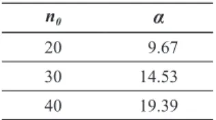
In the following analysis we would like to calculate the influence of the remaining two variables on the marginal contribution α. First, let us analyze how factor α is chan-ged for different values of n and with constant expected income growth i0=3%.
Table 2 Values of
α
for different values of n0, and with p0=3% and i0=3%n0 α
20 9.67
30 14.53
40 19.39
From Table (2) we can notice that for a short saving period n the marginal contribu-tion α is small, while for large values of n it is considerably larger and doubles for a sa-ving period twice as long. This means that for long-term sasa-vings the influence of pensi-on fund return pensi-on accumulated savings becomes even more important.
Table 3 Values of αfor different values of i0, and with p0=3% and n0=38
i0 α
2% 19.55
3% 18.41
4% 17.29
From Table (3) we can notice that the marginal contribution α decreases with an in-crease in income growth rate. However, this dein-crease is not significant since for twice as large an income growth rate the factor α is smaller by only 11.6%.
3.2 Marginal contribution to changes in income growth rate
Let us analyze the marginal contribution β of accumulated savings with respect to di-fferent values of n by keeping the expected pension fund return p0 constant and equal to
3%.
Table 4 Values of βfor different values of n0, and with p0=3% and i0=3%
n0 β
20 9.22
30 14.08
40 18.94
From Table (4) we can notice that the influence of income growth rate i on accumu-lated savings increases as the duration of saving period n increases. If someone is going to save for retirement twice as long as planned, then the marginal contribution β doubles. As in the case of marginal contribution α, this means that for long-term savings the influ-ence of income growth rate on accumulated savings becomes more and more important as time passes.
From Tables (2) and (4) we can notice that for the same duration of saving period n the marginal contribution α is larger than the marginal contribution β by approximately the same amount of 0.45. There is an often-repeated claim in the public that pension fund return is by far the most important factor influencing accumulated savings, while the in-fluence of the income growth rate is usually neglected. Here, we can see that the influen-ce of the income growth rate on accumulated savings is just slightly smaller than the in-fluence of pension fund return for durations of saving periods in a range from 20 to 40 years. Therefore, we can conclude the income growth rate is also important for retirement savings, which is dominantly long-term with durations up to 40 years or even more, and that it deserves greater attention in the analysis of pension plans.
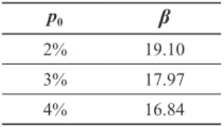
Table 5 Values of βfor different values of p0, and with i0=3% and n0=38
p0 β
2% 19.10
3% 17.97
4% 16.84
From Table (5) we can notice that marginal contribution β is decreases with an incre-ase in pension fund return. However, the decreincre-ase in the value of β is relatively small in a wide range of pension fund returns that are characterized either by a very conservative or a moderately aggressive portfolio.
3.3 Marginal contribution to changes in duration of saving period
Let us observe the marginal contribution γ for different values of pension fund return p with constant income growth rate i.
We can observe from Table (6) that there is no major influence of pension fund return on marginal contribution γ, which describes the sensitivity to the duration of the saving period.
Table 6 Values of γfor different values of p0, and with i0=3% and n0=38
p0 γ
2% 5.13
3% 5.59
4% 6.10
At the end, let us observe how marginal contribution γchanges with variations in the income growth rate i while pension fund return p is held constant.
Table 7 Values of γfor different values of i0, and with p0=3% and n0=38
i0 γ
2% 5.13
3% 5.59
4% 6.10
However, if we analyze the reference point where the duration of the saving period is very short, then the marginal contribution to changes in the duration of saving period γ is significantly larger than other marginal contributions. For example, if we take 10 years as the duration of the saving period and values p0=3% and i0=3%, we obtain
α
=4.82 and β=4.37 while γ is equal to 12.96. Generally, the marginal contribution to changes in the duration of the saving period rapidly decreases with an increase in the saving period. The-refore, we can conclude that it is unfavorable to plan for pension savings in a defined con-tribution system if its duration is too short, since then the sensitivity to the duration of the saving period is extremely large. According to this study it is now understandable why there are problems with the annuities of those insured persons who stayed in the 2nd pillarfor too short a period of time.
Table 8 Comparison of α,βandγfor n0=37
(p, i) α β γ
(2%, 2%) 18.10 17.65 4.68
(2%, 3%) 17.01 18.56 5.20
(2%, 4%) 15.95 19.42 5.77
(3%, 2%) 19.01 16.56 5.20
(3%, 3%) 17.93 17.48 5.66
(3%, 4%) 16.86 18.37 6.17
(4%, 2%) 19.87 15.50 5.77
(4%, 3%) 18.81 16.41 6.17
(4%, 4%) 17.76 17.31 6.62
Table 9 Comparison of α,βandγfor n0=38
(p, i) α β γ
(2%, 2%) 18.59 18.14 4.61
(2%, 3%) 17.45 19.10 5.13
(2%, 4%) 16.32 20.02 5.70
(3%, 2%) 19.55 16.99 5.13
(3%, 3%) 18.41 17.97 5.59
(3%, 4%) 17.29 18.91 6.10
(4%, 2%) 20.46 15.87 5.70
(4%, 3%) 19.35 16.84 6.10
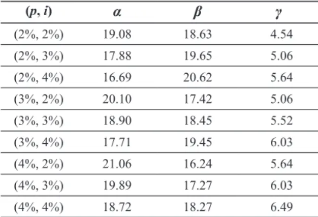
Table 10 Comparison of α,βandγfor n0=39
(p, i) α β γ
(2%, 2%) 19.08 18.63 4.54
(2%, 3%) 17.88 19.65 5.06
(2%, 4%) 16.69 20.62 5.64
(3%, 2%) 20.10 17.42 5.06
(3%, 3%) 18.90 18.45 5.52
(3%, 4%) 17.71 19.45 6.03
(4%, 2%) 21.06 16.24 5.64
(4%, 3%) 19.89 17.27 6.03
(4%, 4%) 18.72 18.27 6.49
3.4 Comparison of marginal contributions α,βandγ
In this section we compare marginal contributions α,βandγaround previously set up reference values in order to determine their influence on changes in accumulated sa-vings. Since we have a three dimensional parametric space, we show three different ta-bles in which the duration of saving period n is held constant, and pension fund return p and income growth rate i are variable. Note that for any other arbitrary values of parame-ters in a range shown in these tables, it is possible to interpolate between them in order to obtain proper values of marginal contributions α,βandγ.
From Tables (8), (9) and (10) we observe that the duration of the saving period makes the smallest marginal contribution to changes in accumulated savings in every point aro-und the reference point (p0, i0, n0). Also, we notice that αis larger then βin those points
where p is nearly equal to i, i.e., when pension fund return is equal to income growth rate, the marginal contribution of the pension fund return is larger then the marginal contribu-tion of the income growth rate. It is important to mencontribu-tion that this difference is rather small and that in general studies we should not overlook the importance of the income growth rate. Furthermore, if the income growth rate is larger then the pension fund return by one percentage point, then the influence of the income growth rate on accumulated savings is larger than the influence of the pension fund return. Also, if the duration of the saving pe-riod increases, then its influence on accumulated savings decreases, while the influences of pension fund return and income growth rate become larger.
At the end, let us notice changes in accumulated savings if pension fund return p is held constant while the other two parameters are variable around the reference point (p0,
Table 11 Changes in accumulated savings for p0=3%
n \ i 2% 3% 4%
36 -0.18 -0.06 0.11
37 -0.16 -0.03 0.17
38 -0.14 0.00 0.23
39 -0.12 0.04 0.29
40 -.010 0.08 0.37
In Table (11) we listed changes of accumulated savings as measured in percentage points with respect to the reference point for different values of i and n. Suppose we are interested in finding out by how much an insured person has to increase her income growth rate in order to retire one year earlier and to accumulate the same amount of savings (howe-ver, not the same annuity). If an insured person, e.g., has worked for 39 years instead of 38 years, and his or her income growth rate is equal to 3%, then the accumulated savings will increase by 0.04 or 4%. However, if the same insured person has worked 38 years, and their income growth rate increases from 3% to 4%, then the accumulated savings will increase even more – around 0.23 or 23%, as determined by the linear approximation of calculating marginal contributions. If we use exact values from equations (2.2) and (2.3), then the increase of accumulated savings will be something smaller and equal to 20%.
Although this analysis can help us to determine the required set of parameters to ma-intain the same amount of accumulated savings for earlier retirement, the annuities will not be the same. That is, if we decrease the duration of the saving period for an insured person, we also increase the person’s life expectancy since we decrease the age at the mo-ment of retiremo-ment. Therefore, the annuity is expected to be paid for longer periods, which decrease its amount. A decrease in the annuity is not linear since the following equation is not valid: e=ex+1 +c, where c is some constant value, and ex is the life expectancy of a
person with age x. With the increasing age of an insured person, the changes in life expec-tancy between adjacent years of age also increase. More precisely, as an insured person’s age increase, his or her life expectancy drops more rapidly. For example, a male aged 56 has a 3.87% lower life expectancy than a male aged 55, while a male aged 66 has a 4.83% shorter life expectancy than a male aged 65 (Actuarial Tables, 1998). The consequence is that with increasing age the difference between annuities of adjacent ages increases. Note that in order to calculate the necessary parameters for having the same annuity for earlier retirement, it is necessary to include in the analysis the phase of annuity payment throu-gh the pension insurance company, which determines the annuities on actuarial principles, i.e. based on the age of the insured person. Moreover, since the total pension from the new pension system is also determined by the 1st pillar pension scheme (Pay-As-You-Go), it
3.5 Influence of an increasing contribution rate for the 2nd pillar
In this chapter we described an approximate model for calculating accumulated sa-vings in a defined benefit pension system depending on three main factors: duration of the saving period, pension fund return and income growth rate. In this section we analy-ze how the change in the contribution rate for the 2nd pillar influences accumulated
savin-gs by using a simple approximation. We assume an annual increase in the contribution rate with a growth rate j, and that it lasts for the entire saving period. Although the assu-med path to increase contributions in the 2nd pillar is over-simplified, it helps us to take
advantage of our study in order to determine the influence of changes in the contribution rate on accumulated savings.
Let us denote by d the corresponding index of growth in the contribution rate:
d= +1 j. (21)
If the contribution R is paid at the end of a month, then the expected amount of accu-mulated savings C after n years of investments is equal to:
C R r
r
r q d
r q d
n n
= −
− −
−
⋅ ⋅ ⋅
⋅
1 1
1 12/
( )
. (22)
If we define a new variable q’=q·d, and calculate accumulated savings as in equation (2) at a point (r, q’, n), such expression can be seen to be identical to equation (22). The-refore, we can assume that an increase in the contribution rate is equivalent to an increa-se in the income growth rate. We would like to know is the magnitude of the influence of an increased contribution rate on the marginal contributions of various parameters. For that purpose we define marginal contributions α',β'andγ'and associate them with mar-ginal contributions α,βandγ:
α'=α( , ', )r q n , (23)
β' β
' '
= 1 = 1 =
0 0
C C
q C
C q
q
q d
⋅∂
∂ ⋅
∂
∂ ⋅
∂
∂ (r,q',n)⋅ , (24)
γ'=γ( , ', )r q n . (25)
Notice that marginal contribution β is scaled by factor d while other marginal contri-butions remained intact.
Let us set up a scenario where the contribution rate for the 2nd pillar is to be
Table 12 Values of α'andβ'with p0=3%, i0=3% and n0=20.
α' 9.59
β' 9.31
By comparing (α',β')and (α,β)in the reference point (3%, 3%, 20) we can conclu-de that an increase in the contribution rate for the 2nd pillar effectively decreases the
mar-ginal contribution of pension fund return and increases the marmar-ginal contribution of inco-me growth rate. From Tables (2) and (4) we already observed that for an equal duration of saving period n the marginal contribution α is larger than the marginal contribution β by approximately the same amount of 0.45, while the difference between marginal con-tributions α'andβ' shown in Table (12) is almost twice as small and equals 0.28. Accor-ding to the proposed scenario of increasing the contribution rate for the 2nd pillar during
the whole saving period, which surely does not represent a realistic scenario due to the very slow dynamics of increases in the contribution rate, we can conclude that the margi-nal contributions of pension fund return and income growth rate are equally important. In a more realistic scenario of increases in the contribution rate for the 2nd pillar, in which
the rate should increase by at least 10% over 10 years, i.e. by 0.5 percentage points per year, we can expect the marginal contribution of income growth rate to be equal to or even higher than the marginal contribution of the pension fund return.
4 Conclusion
In this article we analyzed the standard model for calculating accumulated savings in a defined contribution pension system where the main factors are the duration of the sa-ving period, pension fund return and income growth rate. We used a linear approximati-on to calculate the marginal capproximati-ontributiapproximati-ons of particular parameters, which shows how small changes in the parameters influence accumulated savings. The goal of this sensitivity anal-ysis was to determine the influence of any particular parameter for some reference valu-es of the parameters which are applicable to the 2nd pillar pension scheme in Croatia.
In this article we determined that the marginal contributions for pension fund return and income growth rate considerably increase with the duration of the saving period, and that the difference between these two contributions is approximately equal to 0.45 wha-tever the duration of the saving period. Moreover, these two marginal contributions do not change significantly if we keep the duration of the saving period constant, and the only change is in their mutual relationships. The marginal contribution of the duration of the saving period also slightly depends on changes in the other two parameters.
At the end, we analyzed a simple scenario in which the contribution rate for the 2nd
pillar is increased in equal amounts over the whole saving period. In that case it is possi-ble with a simple adjustment of the previously determined model to calculate new margi-nal contributions for the model parameters. In the example of reference values for para-meters in which we choose 20 years for the duration of saving period, and with the assump-tion of an increase in the contribuassump-tion rate by 5 percentage points in these 20 years of sa-vings, we calculated that the marginal contribution of the income growth rate becomes more important for changes in accumulated savings.
The obtained results for the sensitivity of various parameters in the standard model for calculation of accumulated savings in defined contribution system enable the simpler planning of such a pension scheme at the system and at the individual level. The natural next step in a future analysis is to determine the influence of the risks of various asset cla-sses on achieving expected pension fund return, due to its dominant influence on accu-mulated savings.
LITERATURE
Dimson, E., March, P. R. and Staunton, M., 2009. Credit Suisse Global Investment Returns Yearbook 2009. Zurich: Credit Suisse Research Institute.
Šorić, K., 2000. “Izračun mirovine na temelju individualne kapitalizirane štednje”, Računovodstvo i financije, (5), 75-87.