Factor Analysis, Target Factor Testing and Model Designing of Aromatic Solvent Effect of the Formyl Proton Nuclear Magnetic Resonance Chemical Shift in Para substituted Benzaldehydes

ISSN 1546-9239

© 2010 Science Publications

24

Factor Analysis, Target Factor Testing and Model Designing of

Aromatic Solvent Effect of the Formyl Proton Nuclear Magnetic Resonance

Chemical Shift in Para Substituted Benzaldehydes

Ghazwan F. Fadhil

Department of Chemistry, College of Science, University of Duhok, Duhok, Iraq

Abstract: Problem statement: The variations of formyl proton Chemical Shifts (CS) of p-substituted benzaldehydes in aromatic solvents were investigated. The validity of several physical solvent and empirical solvent scales was examined. Also, to predict dipolarity-polarizability (π*) solvent scale for some aromatic solvents. Model designing was also achieved to rationalize the aromatic solvent effect on the formyl proton CS. Approach: The previously recorded formyl proton CS for p-X- benzaldehydes, with X were NMe2, OMe, OC3H7, H, Br, CHO and NO2 in benzene, toluene, p-xylene,

m-xylene and mesitylene were subjected to Factor Analysis (FA). Target Factor Testing technique (TFT) was performed for several solvent scales namely: Unity, the intrinsic aromatic solvent induced shift of TMS (IASISTMS), f(n), f(d), (n2-1)/(n2+2), (d-1)/(d+2), ET(30) and π*. Iterative TFT was

applied to predict unmeasured (π*) solvent scale for ethyl benzene, n-butyl benzene, sec-butyl benzene, tert-butyl benzene and isopropyl benzene. Results: It has been found that two factors were responsible for the variation in the formyl proton CS. The unity, f(n), (n2-1)/(n2+2), IASISTMS, ET(30)and π*

were real factors. Model designing of the formyl proton CS in benzene, toluene, p-xylene, m-xylene and mesitylene were achieved. The models with lowest root mean square error (RMSE) have shown that Unity is a consistent term. The other term was either IASISTMS or π*. Iterative TFT predicted new π* values for ethylbenzene, n-butylbenzene, sec-butylbenzene, tert-butylbenzene and isopropylbenzene respectively. Conclusion: FA has revealed that two real factors are responsible for the variation of formyl CS in benzene, toluene, p-xylene, m-xylene and mesitylene solvents. TFT has shown to be a powerful technique in predicting new values of the π* solvent scale. Model designing for the formyl proton CS have revealed that the IASISTMS, π* and Unity are the best empirical solvent scales and were better than any physical solvent scales in reproducing the formyl CS. The IASISTMS reflects the dipolarity-polarizabilty of the aromatic solvent. The cofactor of the solvent scale was found to correlate with the σp+ substituent parameter.

Key words: Formyl proton NMR chemical shift, factor analysis, principal components analysis, target factor analysis, aromatic solvent effect,dipolarity-polarizability solvent scale

INTRODUCTION

It is well-known that a solvent exerts an effect on many solvent dependent properties. These solvent-solute interactions can be related to physicochemical scales by constructing a solvent model (Koppel and Palm, 1972). Two types of solvent scales are generally used for modeling: (a) a physical solvent scale such as the dielectric function, the refractive index function or a modified function of both; or (b) the empirical solvent scales, which are derived from a solvent dependent process. There are many empirical solvent scales. A recent comprehensive review (Katritzky et al., 2004) lists 183 solvent polarity scales. We cite the most popular of them, i.e., Reichardt (1979) solvent polarity

parameter ET (30) and Taft’s solvent

dipolarity-polarizability scale π* (Kamlet et al., 1977).

CODESSA programme for 350 solvents has enabled direct calculation of predicted values for any scale for any previously unmeasured solvent. Principal Component Analysis (PCA) for 40 solvent scales of 40 solvents has been carried out (Katritzky et al., 1992). The results allowed a comparison of both solvent scales and characterization of individual solvents. However, aromatic solvent empirical scales have received very limited investigation and there have been missing π* values for these aromatic solvents. The original article (Kamlet et al., 1977) for the π* solvents also carried few aromatic solvents. Bertra’n and Rodri’guez (1983a) measured the chemical shift of formyl proton of several p-substituted benzaldehydes in different aromatic solvents. Bertra’n and Rodri’guez (1983b) aims were to derive a scale called the intrinsic aromatic solvent induced shift of the TMS (IASISTMS) proton and gauge the effect of TMS on the linear correlations of the proton of Aromatic Solvent Induced Shift (ASIS). They did not model the aromatic solvent in terms of empirical or physical solvent scales. Factor Analysis (FA) also called PCA and Target Factor Testing (TFT) techniques have proven to be successful in tackling several chemical problems (Malinowski, 2002; Fadhil, 1992; Fadhil, 1993; Altun, 2005; Altun and Koseoglu, 2006). TFT allows the testing of the validity of each solvent scale individually before constructing the model. TFT could also be used to predict unknown values for solvent scales from the experimental data under investigation.

The aim of this study is to target factor test several physical and empirical solvent scales, model the aromatic solvent effect of the formyl proton in para substituted benzaldehydes and predict new π* scale values for unreported aromatic solvents.

MATERIALS and METHODS

The formyl proton CS for p-substituted-benzaldehyds in ppm data were taken from (Bertra`n and Rodri`guez, 1983a). The formyl proton CS in a given solvent was referenced with respect to cyclohexane.

Factor analysis (Malinowski, 2002)can be used to analyze large data sets without relying upon preconceived chemical model. The method is based on expressing a data matrix D into a product of two matrices R and C plus an error matrix E:

D = RC+E (1)

In Eq. 1:

D = An r×c matrix R = An r×n matrix C = An n×c matrix

E = An r×c matrix composed of experimental errors

In other words, each element of the data matrix is assumed to have the form:

n

ik ij jk ik ik ik j 1

d r c e d (n) e

=

=

∑

where, the sum is taken over n factors, eik is the residual

error unaccounted for by the factor model and dik ( n) is

the reproduced data point based on n factors.

The decomposition is readily accomplished by singular value decomposition, which yields:

D = USVT (3)

Where:

U and V = Matrices whose columns contain unit-length eigenvectors associated, respectively, with the R and C matrices

S = A diagonal matrix containing the normalization constants for each pair of row-column eigenvectors

The elements of S are the square roots of the eigenvalues. An eigenvalue, λj, represents the variation

in the data attributed to the associated eigenvectors. The largest set of eigenvectors (λl, λn), also called primary

factors, accounts for the principal components, where the smallest set ((λn+1 to λs), also called secondary

eigenvalues, account for experimental errors: λ1>λ2>……λn >λn+1……>λs

primary | secondary (4)

(components) | (errors)

In eq. 4, s represents r or c, whichever is smaller. The sum of the smallest set of eigenvalues equals the sum of squares of the error (e2ik):

s r c r c

2 2

j ik ik ik

j n 1 i 1 k 1 i 1 k 1

(d (n) d ) e

= + = = = =

λ = − =

∑

∑∑

∑∑

In Eq. 5, dik (n) represents a data point reproduced

using only n primary eigenvectors.

26 s

r c 2

j ik

j n 1 i 1 k 1

e RSD

(r n)(c n) (r n)(c n)

= +

= =

⎛ ⎞

⎛ ⎞ _λ

⎜ ⎟

⎜ ⎟

⎜ ⎟

⎜ ⎟

= =

⎜ ⎟

− − − −

⎜ ⎟

⎜ ⎟

⎜ ⎟

⎝ ⎠ ⎝ ⎠

∑

∑∑

(6)

The right side is the result of applying Eq. 5. The denominator in Eq. 6 represents the degrees of freedom. Expressing RSD in terms of eigenvalues affords a computationally efficient way to evaluate this important quantity.

If a reasonable accurate estimate of the standard deviation is known prior to the factor analysis the number of primary factors can be determined by direct composition to that obtained from Eq. 6. When such information is not available the problem becomes acerbated.

In factor analysis technique, Malinowski and McCue (1981) have defined two functions to detect the significant number of factors in the data matrix. They called them the indicator function IND (Malinowski, 2002) and the reduced eigenvalue function REV (McCue and Malinowski, 1981; Malinowski, 1987) defined by Eq. 7 and 8 respectively:

IND = RE/(c-n)2 (7)

REVj = λj/(r-j+1)(c-j+1) (8)

s

1/ 2 j

j n 1

RE / r(c n)

= +

=

∑

Where:

RE = The real error

λj = The jth smallest eigenvalue (eigenvalue

due to error)

r, c and n = The number of rows, columns such that (r>c) and primary factors in the data matrix respectively

IND function is a function of secondary eigenvalues, the number of rows and columns in the data matrix and the significant number of factors. Hence, the behavior of IND function varies with the number of factors. The number of factors is gradually increased and the corresponding IND function is observed. As the number of factors is increased, the IND function is decreased in value and reached a minimum when the significant number of factors is achieved. REV is a function of secondary eigenvalues and will remain fairly constant for error eigenvalue. Recently Malinowski (2009) has developed a successful method called Determination of Rank by

Median Absolute Deviation (DRMAD) to determine the number of principal factors responsible for a data matrix by direct application to the RSD obtained from principal component analysis. The MAD was defined as:

MAD = median|| xi - median (xi) || (10)

An outlier (xo) is defined if || xo-median (xo)||/MAD>5

Where:

x = Represents RSD

MAD = Ideally suited to determine the set of error eigenvalues

If a primary eigenvalue is added to the set of error eigenvalues, the RSD will become much larger than true RSD. The resulting RSD will be an outlier that can often be identified by MAD analysis. Factor level (n) representing the dividing line between the primary and secondary sets of eigenvalues . A zero in the test column of DRMAD indicates that RSD based on n factors is an outlier. Unity indicates that the associated RSD is not an outlier of secondary set. TFT (Malinowski and Howery, 1980) involves the following matrix transformation:

[D] = [R]abstract[T][T]− 1

[C]abs = [R]transformed[C]transformed (11)

Where:

[T] = An appropriate transformation matrix [T]−1 = The inverse of [T]

[R] and [C] = Being row and column matrices respectively

They are called abstract matrices, because they represent a purely mathematical solution of the problem. The target testing is described as follow:

[R]PFA T = Rpredicted ≈ Rtest (12)

T is the target transformation vector generated from a least-square operation involving the principal factor analysis solution and the individual target being tested as a vector Rtest. If the test vector Rtest is real

factor the predicted vector Rpredicted obtained from last

equation will be reasonably similar to the test vector i.e. it will lie within the experimental error. Otherwise the tested vector will be rejected. The criterion upon which a tested vector is being accepted or rejected was developed also by Malinowski and Howery (1980). TFT was achieved by monitoring the SPOIL function. SPOIL function was defined as in Eq. 11:

Where:

RET = The real error in target factor

REP = The real error in predicted target factor EDM = The real error from the data matrix

According to Malinowski and Howery a SPOIL value between 0 and 3 is an indication of an acceptable factor and a SPOIL value greater than 3 is not acceptable. FA was performed for the covariance matrix of the formyl chemical shift. Standardization was not applied. FA and TFT calculations were performed using FACTANAL computer programme (Malinowski). DRMAD test was performed on MATLAB code computer programme (Malinowski, 2009).

RESULTS AND DISCUSSION

Number of factors: The solvent shifts of formyl proton Chemical Shifts (CS) of seven p-X-benzaldehydes in 10 aromatic solvents are shown in Table 1.

Bertra’n and Rodri’guez (1983a) have noticed that plotting the formyl CS for a given p-X-benzaldehyde against δHx versus δHH for the unsubstantiated

benzaldehyde in 12 aromatic solvents gave a bilinear plot, such that the monoalkyl benzenes form a separate linear plot (for instance, the correlation coefficient for δHNO2 versus δHHwas 0.987). The remaining solvents

form a separate straight line. For that reason, we performed FA to a subgroup of solvents, namely benzene, toluene, p-xylene, m-xylene and mesitylene. Our data matrix is composed of the formyl CS in the above solvents. The p-X-benzaldehydes with X were

NMe2, OCH3, OC3H7 , H, Br, CHO and NO2. Results of

the FA for this matrix are presented in Table 2.

The IND function initially decreased as the number of factors increased, but started to increase as the number of factors exceeded two. The REV function decreased sharply as the number of factors increased

from one to two then stabilized as the number of factors exceeded two. The DRMAD test gives Unity value at two factors. The three methods give a conclusive result that two primary eignevalues are necessary to account for the factor space of the formyl Aromatic Solvent Induced Shift (ASIS). This conclusion is further confirmed by the value of the Real Error (RE) and RSD functions at two factors, which are close to the experimental error 0.005 (Bertra’n and Rodri’guez, 1983a).

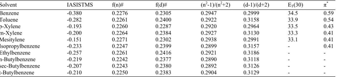
Target factor testing: TFT was performed for several solvent scales at two factors for the same data matrix as the FA results mentioned above. Table 3 lists these solvent scales together with their values. Results of testing are presented in Table 4. The Unity (U) which is equal to one for each solvent, f (n) the refractive index, (n2-1)/ (n2+2) function and the IASISTMS gave the lowest SPOIL values.

This indicates that these solvent scales can be classified as primary factors. The IASISTMS was derived empirically from linear correlation of the ASIS of a group of sensor protons in two fixed aromatic solvents. Several solute systems were used, namely p-X-benzaldehydes, camphor, α-Br-camphor, 5-Xfurfurals, p-X-acetophenones and methyl ketones (Bertra’n and Rodri’guez 1983b).

Table 1: The solvent shifts of the formyl protons of p-X- benzaldeyhde in aromatic hydrocarbon solvents with respect to cyclohexane solventa

Para substituent

--- Aromatic solvent NMe2 MeO C3H7O H Br CHO NO2

Benzene 0.140 -0.119 -0.085 -0.272 -0.456 -0.523 -0.725 Toluene 0.057 -0.162 -0.126 -0.327 -0.500 -0.552 -0.723 Ethylbenzen 0.049 -0.146 -0.126 -0.295 -0.456 -0.514 -0.674 Isopropylbenze 0.043 -0.138 -0.119 -0.272 -0.429 -0.472 -0.627 sec-Butylbenzen 0.023 -0.118 -0.104 -0.220 -0.376 -0.410 -0.556 n-Butylbenzene 0.032 -0.124 -0.108 -0.246 -0.400 -0.436 -0.571 tert-Butylbenzene 0.026 -0.146 -0.125 -0.275 -0.424 -0.473 -0.624 p-Xylene -0.034 -0.224 -0.190 -0.378 -0.541 -0.584 -0.724 m-Xylene -0.018 -0.217 -0.188 -0.371 -0.533 -0.577 -0.735 Mesitylene -0.058 -0.246 -0.225 -0.410 -0.547 -0.602 -0.720

a_{: Data were taken from Bertra’nand Rodri’guez (1983a)}

Table 2: Variation of RE, RSD, IND, REV and DRMAD functions with the number of factors

No. of factors Real error RSD IND function REV function DRMAD

1 4.394×10−2 _4.3360×10−1 _2.746×10−3 _1.789×10−1 _0.000

2 4.980×10−3 _4.7465×10−2 _5.530×10−4 _2.231×10−3 _1.000

3 3.673×10−3 _5.8889×10−3 _9.180×10−4 _2.208×10−5 _1.000

28

Table 3: Values of aromatic solvent scales

Solvent IASISTMS f(n)# f(d)# (n2_-1)/(n2_{+2) (d-1)/(d+2) E}

T(30) π*

Benzene -0.380 0.2276 0.2305 0.2947 0.2999 34.5 0.59 Toluene -0.282 0.2261 0.2400 0.2922 0.3158 33.9 0.54 p-Xylene -0.193 0.2260 0.2287 0.2920 0.2964 33.5 0.43 m-Xylene -0.200 0.2264 0.2384 0.2927 0.3130 33.3 0.41 Mesitylene -0.151 0.2271 0.2302 0.2938 0.2991 33.1 0.41 Isopropylbenzene -0.233 0.2247 0.2399 0.2899 0.3157 - 0.41 Ethylbenzene -0.257 0.2261 0.2416 0.2921 0.3186 - - n-Butylbenzene -0.219 0.2242 0.2377 0.2890 0.3118 - - sec-Butylbenzene -0.207 0.2243 0.2380 0.2892 0.3126 - - t-Butylbenzene -0.210 0.2250 0.2383 0.2904 0.3129 - - #: Timmermans (1965)

Table 4: SPOIL values for different solvent scales and designed models with their RMSE values using benzene, toluene, p-xylene, m-xylene and mesitylene solvents

Tested SPOIL at Combined Root mean Tested SPOIL at Combined Root mean solvent scale two factors solvent scales square error solvent scale two factors solvent scales square error Unity 0.000 π*_{+U 8.620×10}−3 _E

T(30) 1.68 ET (30)+f(n)f 6.100×10−2

f(n)a _{0.000 π}*_{+f (n)}c _9.258×10−3 _{f (d)}b _{3.40 f(n)+U 9.840×10}−2

(n2_-1)/(n2_{+2) 0.000 π}*_+(n2_-1)/(n2₊₂₎d _9.470×10−3 _{(d-1)/( d+2) 4.59 (n}2_-1)/(n2_{+2)+U 9.290×10}−2

IASISTMS 0.600 IASISTMS+U 4.048×10−3 _π* _{1.76 E}

T(30)+U 5.770 x 10-2

a: f(n) = (n2_-1)/(2n2_{+1); b: f(d) = (d-1)/(2d+1), correlation coefficient between combined solvent scales in model; c: (0.380); d: (0.380); e:}

(0.137); f: ( 0.572)

Table 5: Details of solvents models with the lowest RMSE Model (1) Model (2) Model (3) a.IASISTMS+b.U a.π*+b.U a.π*+b.f(n)# Substituent --- --- --- a b a b a b NMe2 -0.8138 -0.1732 1.0820 -0.5105 1.0900 -2.2710

MeO -0.5235 -0.3160 0.6945 -0.5283 0.7035 -2.3690 C3H7O -0.5635 -0.2948 0.7490 -0.5283 0.7579 -2.3500

H -0.5371 -0.4774 0.7140 -0.7000 0.7258 -3.1140 Br -0.3781 -0.6040 0.5026 -0.7607 0.5155 -3.3840 CHO -0.3085 -0.6399 0.4101 -0.7677 0.4231 -3.4160 NO2 0.0014 -0.7251 -0.0020 -0.7245 0.0140 -3.2230 #_{: Similar trend for a and b parameters of model 4 of Table 5}

However, other empirical solvent scales such as π* and ET (30) gave higher but acceptable values of

SPOIL, i.e. lower than three. The physical solvent scales functions, namely (d-1)/(d+2) and f(d), gave SPOIL values higher than three indicating that these tested factors are not target factors.

Model designing of formyl chemical shift in benzene, toluene, p-xylene, m-xylene and mesitylene: In order to construct an empirical model to elucidate the aromatic solvent induced shift, we must choose solvent scales with acceptable SPOIL values. In cases of solvent scales combined with other solvent scales (except Unity), orthogonality of the combined solvent parameters were observed. The combined solvent scales in the designed models and their root mean square errors (RMSE) are presented in Table 4.

Taking in consideration the experimental error is 0.005, only three models gave a RMSE close to the experimental error. One of these models involved the Unity and the IASISTMS scale. The second model

involved Unity and the dipolarity-polarizability solvent scale π*. The third model was constructed by using the dipolarity-polarizability scale π* and f (n) solvent scales. The fourth model involved the π and (n2-l)/(n2+2) solvent scales. Models with a RMSE higher than twice the experimental error were not considered to be successful models for reproducing the formyl CS. It is not a surprise to have model (1) with the lowest RMSE as we commented earlier on the derivation of the IASISTMS. In order to investigate the nature of the IASISTMS scale, we correlated it with π for the same set of solvents used in this study. The correlation coefficient was -0.988, indicating that the IASISTMS solvent scale has a dipolarity-polarizability character. Table 5 presents details of the models with a RMSE less than twice the experimental error.

π* _{prediction for monoalkyl benzene solvents:}

Table 6: Results for predicting π* _{for monoalkylated benzene solvents by TFT technique at two factors}

Etthylbenezene n-Butylbenzne sec-Butylbenzene tert-Butylbenzne No. of --- --- --- --- iterations Predicted π* SPOIL Predicted π* SPOIL Predicted π* SPOIL Predicted π* SPOIL 1 0.4029 60.00 0.3573 38.00 0.3447 30.90 0.3766 40.00 2 0.4680 7.56 0.3983 4.70 0.3813 3.73 0.4218 5.12 3 0.4786 3.59 0.4029 3.10 0.3851 2.65 0.4272 3.36 4 0.4803 3.59 0.4035 3.16 0.3856 2.63 0.4278 3.32

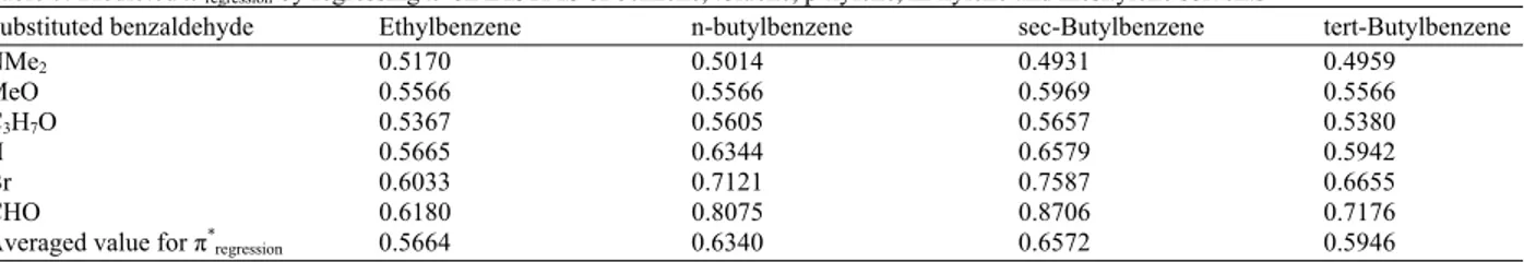
Table 7: Predicted π*

regression by regressing π*on IASTMS of benzene, toluene, p-xylene, m-xylene and mesitylene solvents

Substituted benzaldehyde Ethylbenzene n-butylbenzene sec-Butylbenzene tert-Butylbenzene NMe2 0.5170 0.5014 0.4931 0.4959

MeO 0.5566 0.5566 0.5969 0.5566

C3H7O 0.5367 0.5605 0.5657 0.5380

H 0.5665 0.6344 0.6579 0.5942

Br 0.6033 0.7121 0.7587 0.6655

CHO 0.6180 0.8075 0.8706 0.7176

Averaged value for π*

regression 0.5664 0.6340 0.6572 0.5946

Thus, we constructed a data matrix of the 1H substituent chemical shifts for the previously investigated solvents i.e., benzene, toluene, p-xylene, m-xylene, isopropylbenzene, mesitylene and a monoalkylbenzene solvent with unknown π*. Not only does target factor testing have the ability to test the validity, it also predicts unmeasured values of π* for a certain solvent in the tested factor array. The tested array for π* involved the known values for benzene, toluene, p-xylene, m-xylene, mesitylene, isopropylbenzene and a free floated value of π* which is equal to zero, for the monoalkylbenzene solvent of the unknown π* value. The technique then predicts π* at the correct number of factors, in our case, two. The predicted value of π* for the monoalkylbenzene solvent is then fed back to the tested factor array and another iteration process is conducted until a self consistent value of π* is reached. This usually takes four cycles of iterations. The SPOIL value for the tested π* array is lowest as the π* of monoalkylbenzene solvent approaches the self consistent value. The monoalkylbenzene solvent with the predicted π* is replaced by another one and the free floating iterations are repeated. Table 6 shows the results of the above iterations for the monoalkylbenzenes solvents with unknown π*. The last predicted π*TFT is considered to

be the π*TFT for the given monoalkylbenzenes solvent.

To verify these predicted π*TFT, they were correlated

with the IASISTMS solvent scales, the R2% and F-Fischer being 91.8 and 33.63 respectively for monoalkylated benzene solvents ethylbenzene, n-butylbenzene, sec-n-butylbenzene, tert-butylbenzene and toluene. However, when isopropylbenzene was included the R2%and F-Fischer deteriorated to 86.5 and 25.6 respectively. Thus, we tried to drive a new value

of π* for isopropylbenzene by performing TFT for the following set of solvents: Benzene, toluene, p-xylene, m-xylene, isopropylbenzene and mesitylene. The predicted π*TFT was 0.45 for isopropylbenzene. When

this value was used instead of the derived π* by Kamlet et al. (1977) (0.41), the R2%and F-Fischer for the correlation between π*TFT and the IASITMS became

91.6 and 43.9 respectively for monoalkylbenzene solvents including isopropylbenzene. This correlation coefficient is similar to when isopropylbenzene was excluded from the set of monoalkylbenzenes.

In order to assess the quality of the predicted π*

TFT for the monoalkylbenzene solvents, we made use

of the existing correlation between the π* derived by Kamlet et al. (1977) and the formyl CS of each p-substituted benzaldehyde in the following solvents: Benzene, toluene, p-xylene, m-xylene and mesitylene. Hence, if an unknown π* solvent was added to the above set of solvents a new π*could be derived from each p-substituted benzaldehyde. Newly-derived π* values for a given monoalkylbenzene solvent could be obtained for each substituted benzaldehyde. These π* values for a given solvent could then be averaged to obtain a new single value for π*, which is called π*

regression. Results of such regression are given in Table 7.

Bekarek et al. (1981) derived an equation to calculate the π* scale in terms of the dielectric constant and the refractive index. Equation 1 gives the calculated π*

Bekarek. The calculated π*Bekarek values for ethylbenzene,

n-butylbenzene, sec-butylbenzene, tert-butylbenzene and isopropylbenzene are 0.3903, 0.3726, 0.3736, 0.3736 and 0.3777 respectively. Table 8 gives the R2% and F-Fischer for the correlation between the different π* scales derived in this study and the IASISTMS:

30

Table 8: R2_{% and F-Fischer for correlated solvent scales}

Entry Correlated solvent scales R2_{% F-Fischer Entry Correlated solvent scales R}2_{% F-Fischer}

1 π*

TFT Vs IASISTMSa 91.8 33.63 7 πBek. Vs IASISTMSe 49.0 3.87

2 π*

TFT Vs IASISTMSb 86.5 25.60 8 π*TFT Vs πRega 80.9 12.71

3 π*

TFT Vs IASISTMSc 91.6 43.90 9 π*TFT Vs πRegc 89.9 26.60

4 π*Vs IASISTMSd 92.2 47.26 10 πReg Vs IASISTMSe 60.4 4.58

5 π*

TFT Vs πBekc 42.5 2.95 11 π* Vs IASISTMSf 83.7 41.10

6 π*

TFT Vs πBekb 41.8 2.87 - - - - a_{: Monolkylated benzenes without Isopropylbenzene;} b_{: Monoalkylated benzenes with Isopropylbenzene π}* _{being 0.41;} c_{: Monoalkylated}

benzenes with Isopropylbenzene π* _{being 0.45;} d_{: Benzene, toluene, isopropylbenzene (π}*

TFT = 0.45), p-xylene, m-xylene and mesitylene; e: All

the monoalkylated benzenes; f_{: All the ten solvents in this study with isopropylbenzene (π}*

TFT = 045)

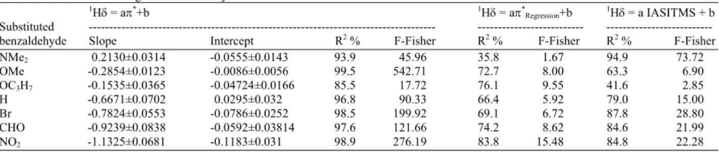
Table 9: Results of modeling 1_{Hδ in monoalkylated benzene solvents}

1_{Hδ = aπ}*_+b 1_{Hδ = aπ}*

Regression+b 1Hδ = a IASITMS + b

Substituted --- ---benzaldehyde Slope Intercept R2 _{% F-Fisher R}2 _{% F-Fisher R}2 _{% F-Fisher}

NMe2 0.2130±0.0314 -0.0555±0.0143 93.9 45.96 35.8 1.67 94.9 73.72

OMe -0.2854±0.0123 -0.0086±0.0056 99.5 542.71 72.7 8.00 63.3 6.90 OC3H7 -0.1535±0.0365 -0.04724±0.0166 85.5 17.72 76.1 9.55 41.6 2.85

H -0.6671±0.0702 0.0295±0.032 96.8 90.33 66.4 5.92 79.0 15.00 Br -0.7824±0.0553 -0.0786±0.0252 98.5 199.92 69.1 6.72 87.8 28.80 CHO -0.9239±0.0838 -0.0592±0.03814 97.6 121.66 74.2 8.62 84.6 21.99 NO2 -1.1325±0.0681 -0.1183±0.031 98.9 276.19 83.8 15.48 84.8 22.28

The most significant correlation was given by the correlation between π*TFT and the IASISTMS for

monoalkylated benzenes (entry 3). Another significant correlation was observed when the solvent set extends to cover mono, di and trialkylated benzenes (entry 11). Entry 11 involves values of π* and π*TFT as independent

variables. Such a significant correlation indicates the coherence between these π* values since two different methods were used to derive them. The correlation with π*

Bekarek was not significant (entries 5-7). However, a

significant correlation between π*TFT and π*Regression was

found, with the correlation becoming more significant when the TFT predicted value of π* for isopropylbenzene was used (entries 8 and 9). This improved correlation gives more confidence to our newly-derived π* for isopropylbenzene.

Model designing of formyl proton chemical shift in

monoalkylated benzenes solvents: In order to

investigate the efficiency of π*TFT, the IASISTMS and

π*

Regression solvent scales for monoalkylated benzenes in

modeling the formyl proton CS, we constructed three models to represent each regression of the formyl proton CS on one of the above solvent scales. Statistical results are presented in Table 9. The R2% and F-Fisher results indicate models which use π* predicted by TFT (π*TFT) are superior to other models. Thus, we have

given the slope and intercept for that model only. The sensitivity of the π*TFT scale as given by the (a)

parameter in Table 5 and 9 were correlated with Hammett’s σp+ substituent constant. Equation 15 gives

the statistical results for such correlation of the σp+ with

the (a) parameter derived from the benzene, toluene, p-xylene, m-xylene and mesitylene sets of solvents-the original sets used to drive π* by TFT for monoalkylated benzene. Equation 16 gives the statistical results for the correlation of σp+ with the (a) parameter derived from

Toluene, n-butylbenzene, sec-butylbenzene, isopropylbenznene and tert-butylbenzene:

σp+ = -1.485 (±0.1997)a+0.8925 (±0.1311)

R2% 95.1 F-Fischer = 57.68 (15) σp+ = -1.130 (±0.0780) a-0.623 (±0.0580)

R2% 98.1 F-Fischer = 209.4 (16) The term which includes the (a) parameter of Table 5 and 9 represents the ASIS because of the electric field which is due to the interaction between the solute and the solvent molecules. The correlation (vide supra) indicates that the intensity of the electric field is not only dictated by the solvent polarity, but also the polarity of substituent i.e., σp+ constant. This may be

attributed to the polarization power effect of the substituent which may influence the overall polarity of the solute molecule.

CONCLUSION

values of the π* solvent scale for ethylbenzene, isopropylbenzene, n-butylbenzene, sec-butylbenzene and tert-butylbenzene. Model designing for the formyl proton chemical shifts in benzene, toluene, p-xylene, m-xylene and mesitylene solvents have revealed that the IASISTMS, π* and Unity are the best empirical solvent scales and were better than any physical solvent scales in reproducing. the formyl CS. The highly significant correlation between IASISTMS and π* implies that the ASISTMS reflects the polarity-dipolarizability character of the aromatic solvent. The polarization power of the substituent and the solvent polarity play a significant role on the intensity of the electric field interaction between the solvent and the substituted p-benzaldehyde.

ACKNOWLEDGMENT

We are grateful to Professor E.R. Malinowski for providing us FACTANAL and DRMAD programmes.

REFERENCES

Ager, I.R. and L. Phillips, 1972. 19F nuclear magnetic resonance studies of aromatic compounds. Part I. The effect of solvents on the chemical shift of fluorine nuclei in para-substituted fluorobenzenes, substituted 4`-fluoro-trans-stilbenes and 4-substituted 3`-fluoro-trans-stilbenes. J. Chem. Soc., Perkin Trans., 2: 1975-1979. DOI: 10.1039/P29720001975

Altun, Y. and F. Koseoglu, 2006. Solute-solvent interaction effects on protonation equilibrium of substituted n-benzylidene-2-hydroxyanilines in aqueous ethanol: The application of factor analysis to solvatochromic parameters and protonation equilibria. Monatsh. Chemistry/Chemical Monthly, 137: 703-706. DOI: 10.1007/s00706-005-0477-6 Altun, Y., 2005. Study of solvent effects on the

protonation of functional group of disubstituted anilines: Factor analysis applied to the correlation between protonation constants and solvatochromic parameters in ethanol-water mixtures. Monatsh. Chemistry/Chemical Monthly, 136: 1993-2006. DOI: 10.1007/s00706-005-0371-2

Bekarek, V., 1981. Contribution to the interpretation of a general scale of solvent polarities. J. Phys. Chem., 85: 722-723. DOI: 10.1021/j150606a023 Bertra`n, J.F. and M. Rodri`guez, 1983a. The effect of

the internal reference on ASIS correlations: 2-The intrinsic ASIS of TMS protons in aromatic hydrocarbon solvents. Org. Magn. Reson., 21: 6-10. DOI: 10.1002/omr.1270210104

Bertra`n, J.F. and M. Rodri`guez, 1983b. The effect of the internal reference on ASIS correlations: 1-Formyl protons of p-X-benzaldehydes Org. Magn. Reson., 21: 2-5. DOI: 10.1002/omr.1270210103 Bukingham, A.D., T. Schafer and W.G. Schneider,

1960. Solvent effects in nuclear magnetic resonance spectra. J. Chem. Phys., 32: 1227-1233. DOI: 10.1063/1.1730879

Dayal, S.K. and R.W. Taft, 1973. Aprotic solvent effects on substituent fluorine nuclear magnetic resonance shifts. III. p-Fluorophenyl-p’-substituted-phenyl systems. J. Am. Chem. Soc., 95: 5595-5604. DOI: 10.1021/ja00798a026

Eliasson, B., D. Johnels, S. Wold and U. Edlund, 1982. On the correlation between solvent scales and solvent-induced 13C NMR chemical shifts of a planar lithium carbanion. A multivariate data analysis using a principal component-multiple regression-like formalism Acta Chem. Scand. B., 36B: 155-164. DOI: 10.3891/acta.chem.scand.36b-0155

Engler, E.M. and P. Laszlo, 1971. New description of nuclear magnetic resonance solvent shifts for polar solutes in weakly associating aromatic solvents. J. Am. Chem. Soc., 93: 1317-1327. DOI: 10.1021/ja00735a001

Fadhil, G.F., 1992. Factor analysis of long range substituent effects on C-13 NMR chemical shifts and target factor testing of different types of substituent parameters Z. Naturforsch, A, A J.

Phys, Sci., 47: 775-80. http://cat.inist.fr/?aModele=afficheN&cpsidt=5359

089

Fadhil, G.F., 1993. Principal component analysis and target testing of substituent effect using carbonyl stretching frequency and 13C NMR chemical shift data matrices. Collect. Czech. Chem. Commun., 58: 385-3. DOI: 10.1135/cccc19930385

Fowler F.W., A.R. Katritzky and R.J.D. Rutherford, 1971. The correlation of solvent effects on physical and chemical properties. J. Chem. Soc. (B), 1: 461- 469. DOI: 10.1039/J29710000460

Kamlet M. J., J. L. Abboud and A.R.W. Taft, 1977. The solvatochromic comparison method. 6. The π* scale of solvent polarities. J. Am. Chem. Soc., 99: 6027- 6038. DOI: 10.1021/ja00460a031 Katritzky, A.R., T. Tamm, Y. Wang and M. Karelson,

1999. a unified treatment of solvent properties. J. Chem. Inf. Comput. Sci., 39: 692-698. DOI: 10.1021/ci980226

32 Katritzky, A., D.C. Fara, H. Yang, K. Tamm, 2004.

Quantitative measures of solvent polarity. Chem. Rev., 104: 175-198. DOI: 10.1021/cr020750m Koppel, I.A., and V.A. Palm, 1972. The Influence of

the Solvent on Organic Reactivity. In: Advances in Linear Free Energy Relationship, Chapman, N.B. and J. Shorter (Eds.). Plenum Press, ISBN: 0306 305666, pp: 203-280.

Malinowski, E.R., 2002. Factor Analysis in Chemistry. 3rd Edn., John Wiley and Sons, New York, ISBN: 0-471-13479-1, pp: 414.

Malinowski, E.R. and D.G. Howery, 1980. Factor Analysis in Chemistry. John Wiley and Sons, New York, ISBN:

Malinowski, E.R., 1987. Theory of the distribution of error eigenvalues resulting from principal component analysis with applications to spectroscopic data. J. Chemometr., 1: 33-40. DOI: 10.1002/cem.1180010106

Malinowski, E.R., 2009. Determination of Rank by median Absolute Deviation (DRMAD)-A simple method for determining the number of principal factors responsible for a data matrix. J. Chemometr., 23: 1-6. DOI: 10.1002/cem.1182 McCue, M. and E.R. Malinowski, 1981, Target factor

analysis of infrared spectra of multicomponent mixtures. Anal. Chim. Acta, 133: 125-136. DOI: 10.1016/S0003-2670(01)93488-9

Reichardt, C., 1979. Empirical parameters of solvent polarity as linear free-energy relationships. Angew. Chem. Int. Ed. Eng., 18: 98-110. DOI: 10.1002/anie.197900981