An approach to reduce mapping errors in the production of
landslide inventory maps
M. Santangelo, I. Marchesini, F. Bucci, M. Cardinali, F. Fiorucci, and F. Guzzetti
CNR IRPI, Via della Madonna Alta 126, 06128 Perugia, Italy Correspondence to:M. Santangelo ([email protected])
Received: 5 June 2015 – Published in Nat. Hazards Earth Syst. Sci. Discuss.: 1 July 2015 Accepted: 31 August 2015 – Published: 22 September 2015
Abstract. Landslide inventory maps (LIMs) show where landslides have occurred in an area, and provide informa-tion useful to different types of landslide studies, including susceptibility and hazard modelling and validation, risk as-sessment, erosion analyses, and to evaluate relationships be-tween landslides and geological settings. Despite recent tech-nological advancements, visual interpretation of aerial pho-tographs (API) remains the most common method to prepare LIMs. In this work, we present a new semi-automatic pro-cedure that makes use of GIS technology for the digitization of landslide data obtained through API. To test the proce-dure, and to compare it to a consolidated landslide mapping method, we prepared two LIMs starting from the same set of landslide API data, which were digitized (a) manually adopt-ing a consolidated visual transfer method, and (b) adoptadopt-ing our new semi-automatic procedure. Results indicate that the new semi-automatic procedure (a) increases the interpreter’s overall efficiency by a factor of 2, (b) reduces significantly the subjectivity introduced by the visual (manual) transfer of the landslide information to the digital database, result-ing in more accurate LIMs. With the new procedure, the landslide positional error decreases with increasing landslide size, following a power-law. We expect that our work will help adopt standards for transferring landslide information from the aerial photographs to a digital landslide map, con-tributing to the production of accurate landslide maps.
1 Introduction
Landslide inventory maps (LIMs) document the type and ex-tent of mass movements in areas ranging from single slopes, or groups of slopes (Cardinali et al., 2001), to regions (e.g. Brabb and Pampeyan, 1972; Antonini et al., 1993; Duman et al., 2005), and even entire states or nations (Delaunay, 1981; Radbruch-Hall et al., 1982; Brabb et al., 1989; Cardinali et al., 1990; Reichenbach et al., 1998; Trigila et al., 2010). LIMs are prepared using a variety of techniques and methods (Guzzetti et al., 2012), including: (i) analysis of archive and historical information (Reichenbach et al., 1998; Salvati et al., 2003), (ii) visual interpretation of stereoscopic aerial pho-tographs (aerial photo interpretation; API) (Guzzetti and Car-dinali, 1989, 1990; Cardinali et al., 1990; Brunsden, 1993; Antonini et al., 2002b; Guzzetti et al., 2002, 2012; Galli et al., 2008; Santangelo et al., 2010, 2013), (iii) visual analy-sis of lidar-derived images (Ardizzone et al., 2007; Van den Eeckhaut et al., 2007; Haneberg et al., 2009; Guzzetti et al., 2012; Razak et al., 2011, 2013), (iv) visual inspection of monoscopic (Marcelino et al., 2009; Gao and Maroa, 2010; Fiorucci et al., 2011; Giordan et al., 2013) and stereoscopic (Fiorucci et al., 2011; Ardizzone et al., 2013; Murillo-García et al., 2015) satellite images, and (v) image-processing tech-niques (Guzzetti et al., 2012) applied to lidar elevation data (Martha et al., 2010; Lu et al., 2011; Stumpf and Kerle, 2011; Van den Eeckhaut et al., 2012) and satellite imagery (Rosin and Hervás, 2005; Borghuis et al., 2007; Yang and Chen, 2010; Mondini et al., 2011a, 2013, 2014; Mondini and Chang, 2014).
(Brunsden, 1993; Guzzetti et al., 2012). In many areas, aerial photographs (APs) are the only source of landslide informa-tion in the period between the 1920s and 1973, when the im-ages captured by the first Landsat satellite became available (McDonald and Grubbs, 1975; Sauchyn and Trench, 1978).
Production of LIMs through API is known to be a subjec-tive and error-prone operation (Guzzetti et al., 2012; Jack-son et al., 2012). The quality of the final map depends on multiple factors, including the experience and skills of the photo interpreter(s), the scale of the APs and of the base map used to prepare the inventory, and the complexity of the ter-rain (Carrara et al., 1992; Ardizzone et al., 2002; Galli et al., 2008; Jackson et al., 2012). A crucial – and underestimated – source of error that influences the quality of a LIM lays in the transfer of information from the original APs used to recognize demarcate the landslides, to the base map used to produce the LIM (Marchesini et al., 2013, Santangelo et al., 2015a). Most commonly, the transfer of information from the APs to the (digital or paper) map is performed visually. To the best of our knowledge, no attempt has been made to quan-tify the error introduced by the visual transfer of the landslide information from the APs to the base map, and to investigate technological alternatives to the visual transfer that may re-duce the mapping errors, contributing to an improvement of the quality of LIMs.
We present a new semi-automatic GIS procedure for the digitization of landslides and other geomorphological infor-mation obtained through API. We test the new procedure in an area near Taormina, Sicily, where landslides are abundant. In our test area, we compare two LIMs obtained using a con-solidated manual procedure for preparing the inventory and the new semi-automatic procedure, and we discuss advan-tages and drawbacks of the new method compared to the tra-ditional approach.
2 Study area and materials
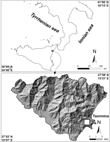
For our experiment, we selected a 93 km2 area along the NE coast of Sicily, near Taormina (Fig. 1). In the area, evation ranges from sea level to 1187 m, with a mean el-evation of 410 m computed from a 2 m×2 m digital ele-vation model (DEM). Terrain slope ranges between 0 and 88◦, with an average of 41◦, and most of the slopes face
towards SSW. Most of the area is drained by the Alcantara River that flows into the Ionian Sea and is characterized by a deep canyon cut into lava flows of the Etna Volcano. A W–E-trending antiformal ridge shapes the morphology of the area (APAT, 2008). Conglomerate, sandstone, and clay per-taining to the Capo D’Orlando Flysch crop out along the SE limb of the ridge. Metamorphic rocks, mainly phyllites and massive and layered carbonate rocks, crop out on the ridge top, and basalt is present in the canyon carved by the Alcantara River. The composite lithological assemblage and the complex structural setting control the morphology of the
Figure 1. Location map. Shaded relief was produced from a 2 m×2 m lidar DEM.
slopes, and the location, type, abundance, and pattern of the landslides. Large, deep-seated landslides and “sackung-type” features (Di Maggio et al., 2014) are most common where metamorphic rocks crop out. Slides, earthflows, complex and composite landslides, and large debris flows are abundant where flysch rocks crop out. In places, hard rocks (carbonate, basalt) form steep, locally overhanging walls that represent the source areas of rock falls, topples, and minor rockslides.
For the study area, the following materials were avail-able to us: (i) a topographic base map at 1 : 10 000 scale, (ii) a 2×2 m resolution DEM obtained from a lidar survey, (iii) a colour orthophoto map with a ground sampling dis-tance (GSD) of 0.25 m, and (iv) 12 black and white aerial photographs (APs) taken on 7 July 2005 at a nominal scale of 1 : 28 000. The APs were 23 cm×23 cm in size, each cov-ering an area of approximately 34 km2, and were taken using an aerial “WILD” camera with a focal length of 153.64 mm. The side overlap between two adjacent APs is about 70 %, and the strip overlap about 20 %.
3 Production of a landslide inventory map
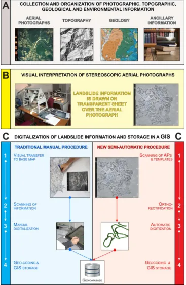
Figure 2.Description of the process of landslide mapping based on the interpretation of the aerial photographs (API).(a)Information useful to the interpretation is collected and organized. (b)Aerial photographs are interpreted using a stereoscope. Landslide and the-matic information is drawn on a transparent plastic sheet (tem-plate) placed over the photographs. (c)Information is digitalized and stored in a GIS. The blue side and arrows show four steps of the consolidated (traditional) manual procedure. The red side and connectors show four steps of the new semi-automatic procedure.
the visual analysis of the stereoscopic APs using a stereo-scope, to the storage of the landslide information in a GIS. Based on our experience, and the production of LIMs for more than 4×10⁵km2 in different physiographical and cli-matic settings in Italy (Antonini et al., 1993, 2002b; Ardiz-zone et al., 2012; Cardinali et al., 2001; Guzzetti and Car-dinali, 1989; Santangelo et al., 2015a), and elsewhere in the world (e.g. Cardinali et al., 1990), we identify three main steps for the production of a LIM (Fig. 2).
First, (step A in Fig. 2) topographic, morphological, ge-ological, and environmental data and information useful for the recognition of the landslides are collected and organized. Next, (step B, in Fig. 2) the available stereoscopic APs are
type (Cruden and Varnes, 1996), relative age (Santangelo et al., 2013), and estimated depth of the landslide. An expected degree of confidence in the recognition can also be attributed to each landslide, or other recognized geomorphological fea-tures (Razak et al., 2012). The interpreter draws the landslide and the additional thematic information detected on the APs on a transparent plastic sheet (template) placed over the AP using fine-scale (0.3 mm, or smaller) colour felt pens. Next, (step C, in Fig. 2) the information shown on the transpar-ent plastic sheet is transferred to the base map, and stored in a GIS. This can be performed using a consolidated manual procedure, or the new semi-automatic procedure proposed in this study (Fig. 2).
3.1 Manual procedure
The manual procedure consists of the following four sub-steps (Santangelo et al., 2012; Marchesini et al., 2013). First, the information drawn on the plastic sheets placed over the APs (Fig. 3a) is transferred visually (re-drawn) to a sec-ond undeformable plastic sheet placed over the topographic base map (Fig. 3b). In this sub-step, all the topographic dis-tortions present in the AP – the result of the conical view of the AP – are adjusted visually to match the undistorted (projected) topographic map. Second, the undistorted plas-tic sheet is scanned – typically using a large-scale (A0 for-mat) scanner, imported as a raster file into a GIS, and geo-referenced. Third, the landslide and the thematic informa-tion is transformed from raster to vector format (vectoriza-tion) using automatic, semi-automatic, or manual methods. Fourth, the single vector elements, each representing a land-slide or a portion of a landland-slide (e.g. a landland-slide escarpment, a landslide boundary), or a morphological or geological fea-ture (e.g. fault traces, trenches) are assembled in single or in multiple vector features. Lastly, each landslide feature is coded (labelled) with the appropriate landslide information, and stored in a GIS in single or multiple layers (Fig. 3c). When multiple layers are used, the different layers can show landslides of different types, or of different ages or periods (Santangelo et al., 2013, 2014).
Figure 3. Main steps of the consolidated manual procedure. (a)Photo-interpreted template obtained through API.(b)Thematic information visually re-drawn on a transparent plastic sheet placed over a topographic base map.(c)Landslide information imported in the GIS, vectorized, and geocoded.
smaller number of reference points on the topographic map compared to the AP, (iv) the quality of the topographic map, and (v) the complexity of the terrain. The manual method is time-consuming (Galli et al., 2008), and the quality of the LIM depends largely on the ability of the operator to transfer the mapped landslide and thematic information from the AP to the base map correctly.
3.2 Semi-automatic procedure
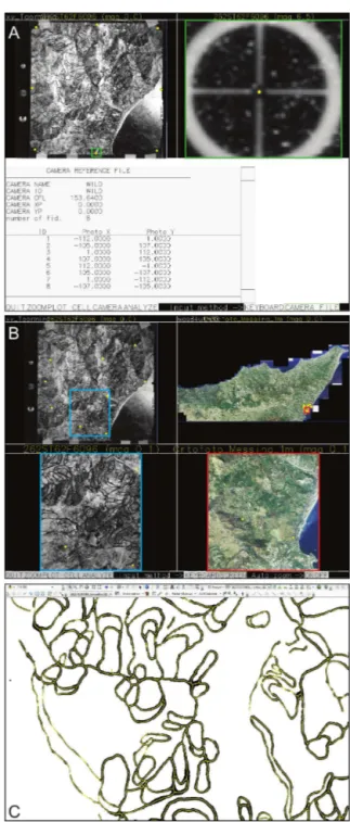
We propose a new, semi-automatic procedure to transfer the landslide and the thematic information recognized in the APs to the topographic base map. The procedure consists of the following four sub-steps (Fig. 2). First, the single AP and the associated plastic sheets showing the landslide and the-matic information are scanned. Three separate scans are pre-pared, including: (i) a grey-tone (8-bit) image of the AP with the plastic sheet (Fig. 4a), (ii) a black and white (1-bit) im-age of the plastic sheet without the AP (Fig. 4b), and (iii) a colour (24-bit) image of the plastic sheet, also without the AP (Fig. 4c). The three scanned images are stored in the GRASS GIS as an imagery group in a project with Carte-sian coordinates (i.e., a generic (x,y) mapset). Second, the imagery group is orthorectified using the grey-tone (8 bit) scanned image of the AP and the associated plastic sheet for the interior and the exterior orientations of the AP, and of the landslide and thematic information. Third, the landslide and the thematic information shown in the scanned plastic sheet is transformed from raster to vector format, automat-ically. Fourth, the individual vector elements are assembled in single or in multiple vector features, each representing e.g. a landslide or a portion of a landslide, or other thematic in-formation. Lastly, the landslide/thematic features are manu-ally labelled with the appropriate information, and stored in the GIS in single or multiple layers (Fig. 3c). To code the individual vector features, we use the 24-bit colour image, using the colours shown in the original (colour) plastic sheet (Fig. 4c).
Figure 4.Input layers (scanned aerial photograph and template) re-quired for the application of the orthorectification procedure.(a) 8-bit grey-tone image of the aerial photograph and its interpreted tem-plate.(b)1-bit black and white image of the interpreted template. (c)24-bit colour image of the interpreted template.
Figure 6. (a)Scatter plot of residuals alongx(µ) andy(ν)for 63 GCPs (different from the GCPs used for the exterior orientation) achieved by orthorectification of the aerial photographs. 68 % (1σ, green ellipse) ofµ–νdata points is smaller than 1.9 and 3.8 m, respectively. 95 % (2σ, red ellipse) ofµ–νdata points is smaller than 3.0 and 6.6 m, respectively. 99 % (3σ, blue ellipse) ofµ–νdata points is smaller than 4.4 and 7.8 m, respectively.(b)Scatter plot of residuals alongx(µ) andy(ν) showing the co-registration of the orthophotograph used for the exterior orientation of the aerial photographs, and the contour line topographic base map used for the visual transfer (Fig. 3b). For both plots, on the right and upper side of the plots, the box plots of the residuals are displayed. Data concentration ellipses of 1, 2, and 3σ are shown. All data concentration ellipses computed giving less weight to the outliers.
et al., 2011). For the interior orientation, the coordinates of the eight fiducial marks were associated using the centre of symmetry of the AP as the origin. For the exterior orienta-tion (Fig. 5b), the i.ortho.photo module requires that a suf-ficient number of ground control points (GCPs) are placed on the AP. In the literature, 16 GCPs are considered suf-ficient if each GCP is placed with an accuracy of 1/3 of the pixel size (Bernstein, 1983; Rocchini et al., 2011), and if the GCPs cover the entire AP avoiding clustering effects. For our experiment, 16–20 GCPs were selected in each AP. Lastly, i.ortho.photo requires a number of output parameters, including the resolution (usually metres per cell/pixel width or length) of the orthorectified image and the interpolation method (e.g. nearest neighbour, bilinear, bicubic) used to re-sample the pixels of the scanned images to the target grid of a given coordinate reference system. The orthorectified images are exported as GeoTIFF files, for subsequent vectorization and coding of the landslide and thematic information.
For the automatic vectorization of the single orthorecti-fied images we used the ArcScan extension of ArcMap™ (ArcGIS®10). The software uses a raster layer (1-bit) of the interpreted template (i.e., an orthorectified image showing the thematic information only, Fig. 5c) as input. The indi-vidual vector features (points, lines, polygons) are cleaned topologically, and then stored in shape files. The attribute ta-ble is then compiled with the appropriate landslide/thematic information using a pre-defined legend.
3.3 Accuracy of the orthorectification
For the rectification of APs, Rocchini et al. (2011) have shown that a robust orthorectification algorithm provides bet-ter results than rectifications techniques that do not use dig-ital terrain information (i.e., a DEM). We adopted the algo-rithm described by Rocchini et al. (2011) and implemented in the i.ortho.photo module of GRASS GIS (GRASS de-velopment team, 2012). Fig. 6a shows measures of the co-registration accuracy of the APs and the orthophotograph used for the exterior orientation. For 63 GCPs (different from the GCPs used for the exterior orientation), we obtained a to-tal root-mean-square error (RMSE) of 5 m, and a 3σ data concentration ellipse < 10 m along thex axis and theyaxis. Considering that the graphical error for an AP at 1 : 28 000 scale is 5.6 m (where the graphical error is 0.2 mm×28 000), and the (nominal) width of the felt pen used to draw the land-slide information on the plastic sheets was 0.3 mm, corre-sponding to 8.4 m at the scale of the APs, we conclude that the semi-automatic orthorectification method is suitable for the production of a LIM, at 1 : 10 000 scale.
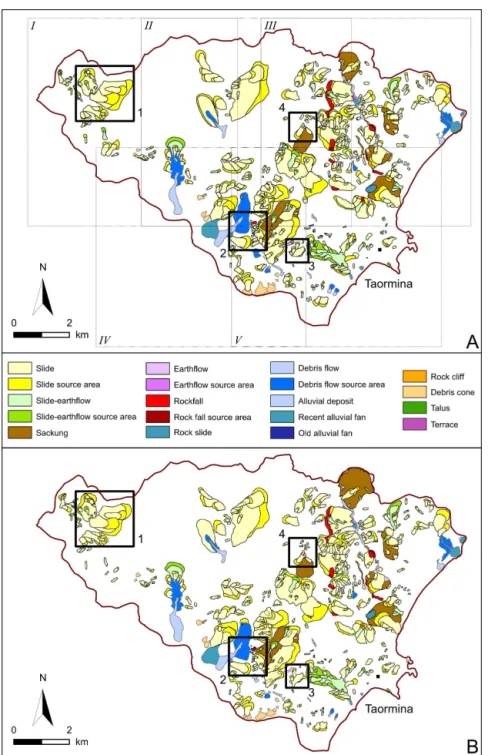
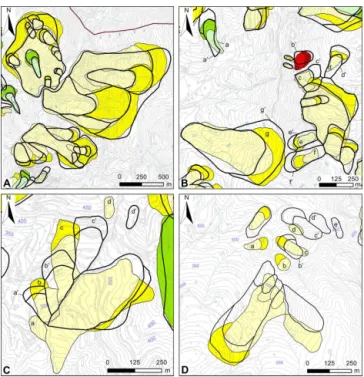
Figure 7.Landslide inventory maps (LIMs) obtained using(a)the consolidated manual procedure, and(b)the new semi-automatic procedure. Bold black boxes numbered from 1 to 4 indicate the four areas shown in Fig. 8 and named from A to D. Thin line boxes with Roman numerals show the areas covered by the five complete stereograms for which the API was carried out.
6.2 m, which reveal a good co-registration between the or-thophotograph used for the exterior orientation of the APs, and the topographic base map used as reference for the man-ual procedure. The good co-registration accuracy allows for the comparison between the LIMs produced using the man-ual and the semi-automatic procedures.
4 Results
Figure 8. Visual comparison of the two inventory maps result-ing from the two different procedures. Black lines are landslides mapped using the consolidated manual procedure. Coloured poly-gons are landslides mapped using the semi-automatic procedure. The four images (bold black boxes in Fig. 7) show situations where: (a)mapping agreement is substantially acceptable,(b)positioning of the landslides is acceptable but not the size,(c)positioning of the landslide is not acceptable, and(d)mapping agreement is very poor, and commission and omission errors occur. Lower-case letters refer to the corresponding landslides mapped using the semi-automatic and the manual (lower-case letters with apex) procedure. See text for explanation.
GIS. The second landslide map (map B, Fig. 7b) was pre-pared by adopting the new semi-automatic method to trans-fer the information from the APs to the base map, and in the GIS. Availability of two maps covering the same area and showing the same landslides allows for qualitative and quan-titative comparisons of the maps. Since the differences in the two maps lay in the method used to transfer the information from the APs to the GIS, analysis of the differences allows us to evaluate the performances of the two methods, outlining advantages and limitations.
We performed an analysis of the mismatch between the in-ventories resulting from the manual and the semi-automatic methods. Figure 8 shows a qualitative comparison of the two LIMs in four areas (black boxes in Fig. 7) that we consider representative of different, typical mapping conditions. Vi-sual inspection of Fig. 8a reveals an overall agreement be-tween the two maps, with local variations dependent on the size of the landslides. In Fig. 8b, there is a good agreement in the geographical location of the single landslides, but the size of some of the landslides differs, locally significantly. Some of the mapped landslides (a′, c′–g′ in Fig. 8b) are
larger in map A and smaller in map B, indicating a system-atic overestimation of the size of the landslides when trans-ferring the landslide information visually. Conversely, land-slideb′(map A) is smaller than the corresponding landslide b(map B), mapped using the semi-automatic procedure. In-spection of Fig. 8c reveals that, with a few exceptions, the size (area) of the landslides shown in the two maps is very similar, but the geographical position of some of the land-slides varies significantly. In particular, the corresponding landslidesaanda′andd andd′do not overlap. Landslides c and c′ and b and b′ overlap partially but their position
does not correspond entirely. Finally, Fig. 8d shows an area where the agreement between the two maps is very poor. In this area, both the size (extent) and the geographical location of some of the landslides are affected by very large errors (e.g. landslidesb andb′,c andc′, and d andd′). In
addi-tion, Fig. 8d shows that one landslide shown in map A (i.e., e′) is not present in map B and, vice versa, landslide a in
map B is not shown in map A. Should we consider map B (prepared through the semi-automatic procedure) as the ref-erence (“true”) map, polygone′would be considered a
com-mission error and polygona an omission error. The differ-ences between the two maps are the result of modifications introduced by the interpreter when transferring the informa-tion manually from the AP to the base map. The operator introduces the (rare) changes locally, in the attempt to adjust the landslide mapping to the local topographic setting shown by the base map.
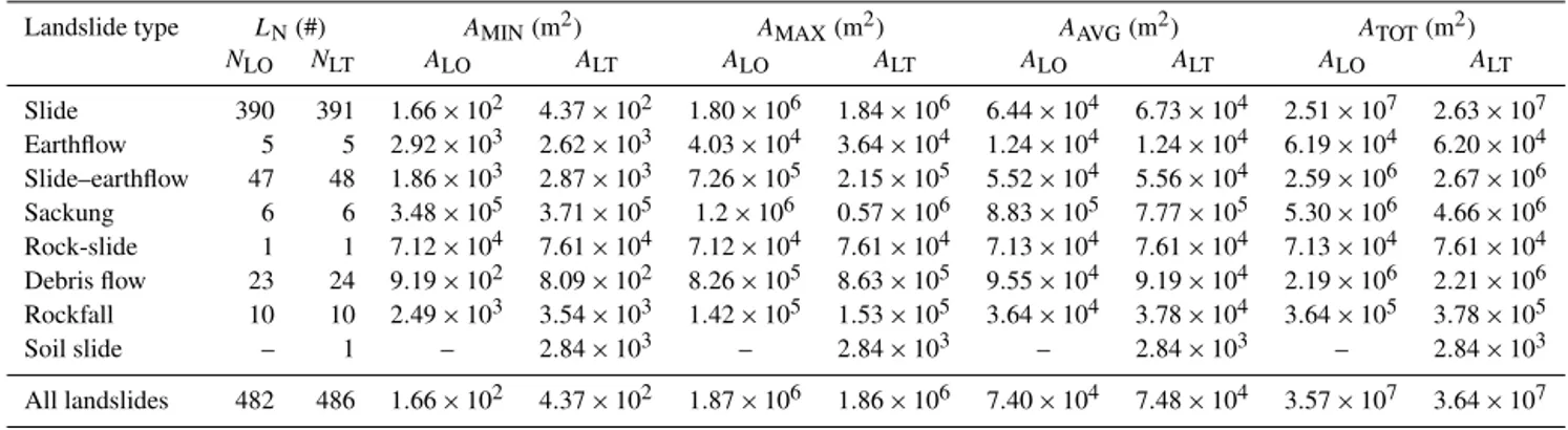
Table 1 summarizes statistics of landslide area (size) for the two LIMs. The smallest landslide in map A is a slide withAL=4.37×10²m2. The same landslide in map B has AL=3.77×10²m2 (a difference of 60 m2). The smallest landslide in map B is a slide withAL=1.66×10²m2. The corresponding landslide in map A hasAL=7.07×10²m2 (a difference of 95 m2). The largest landslide in map B is a sackung withAL=1.87×10⁶m2. In map A, the same sack-ung hasAL=1.86×10⁶m2, revealing a difference of 104m2 (0.5 %) in size. In map A, obtained using the manual proce-dure, the average landslide area isAL=7.48×10⁴m2, and in map B, obtained by carrying out the semi-automatic proce-dure, the average landslide area isAL=7.40×10⁴m2. This is a reduction of 1.1 % of the average landslide area. The total landslide area isALT=3.74×10⁷m2for map A, and ALT=3.57×10⁷m2 for map B. The reduction in the total landslide area, 1.7×10⁶m2, is not small (4.5 %) and con-ditions the percentage of landslide area (landslide density), which is 39.1 % for map A (manual procedure) and 38.4 % for map B (semi-automatic procedure).
ap-NLO NLT ALO ALT ALO ALT ALO ALT ALO ALT
Slide 390 391 1.66×10² 4.37×10² 1.80×10⁶ 1.84×10⁶ 6.44×10⁴ 6.73×10⁴ 2.51×10⁷ 2.63×10⁷
Earthflow 5 5 2.92×10³ 2.62×10³ 4.03×10⁴ 3.64×10⁴ 1.24×10⁴ 1.24×10⁴ 6.19×10⁴ 6.20×10⁴ Slide–earthflow 47 48 1.86×10³ 2.87×10³ 7.26×10⁵ 2.15×10⁵ 5.52×10⁴ 5.56×10⁴ 2.59×10⁶ 2.67×10⁶
Sackung 6 6 3.48×10⁵ 3.71×10⁵ 1.2×10⁶ 0.57×10⁶ 8.83×10⁵ 7.77×10⁵ 5.30×10⁶ 4.66×10⁶
Rock-slide 1 1 7.12×10⁴ 7.61×10⁴ 7.12×10⁴ 7.61×10⁴ 7.13×10⁴ 7.61×10⁴ 7.13×10⁴ 7.61×10⁴
Debris flow 23 24 9.19×10² 8.09×10² 8.26×10⁵ 8.63×10⁵ 9.55×10⁴ 9.19×10⁴ 2.19×10⁶ 2.21×10⁶ Rockfall 10 10 2.49×10³ 3.54×10³ 1.42×10⁵ 1.53×10⁵ 3.64×10⁴ 3.78×10⁴ 3.64×10⁵ 3.78×10⁵ Soil slide – 1 – 2.84×10³ – 2.84×10³ – 2.84×10³ – 2.84×10³
All landslides 482 486 1.66×10² 4.37×10² 1.87×10⁶ 1.86×10⁶ 7.40×10⁴ 7.48×10⁴ 3.57×10⁷ 3.64×10⁷
Figure 9.Comparison of the inverse-gamma (Malamud et al., 2004a) probability density function (pdf) computed for map A and map B. (a)pdf of the inventory obtained by the manual method (map A).(b)pdf of the inventory obtained by the orthorectification method (map B). (c)Enlargement of(a), and(d)enlargement of(b)are provided for aiding visual comparison of the two distributions.
proximated by the double-Pareto (Stark and Hovius, 2001) or the inverse-gamma (Malamud et al., 2004a) functions. Using specific software (Rossi et al., 2009) we determined p(AL)for the two inventories. Results are shown in Fig. 9a, c and b, and d that portray the inverse-gamma approxima-tion top(AL)for map A (manual method) and map B (semi-automatic method), respectively. Comparison of Fig. 9a, c
Table 2.Comparison of scaling exponent (alpha) and rollover (size of the most abundant landslide) for the probability distribution func-tions computed for map A (manual method) and map B (semi-automatic method). Best fits computed through maximum likeli-hood estimation.
α+1 Rollover (m2)
Map A 2.064 6397
Map B 2.020 5326
We obtained an additional quantitative analysis of the dif-ferences between the two inventories modifying the mapping error indexEproposed by Carrara et al. (1992), and used e.g. by Ardizzone et al. (2002) and by Galli et al. (2008). The in-novation of our work was to calculate the positioning error indexEifor each pair of corresponding landslides in the two inventories:
Ei=
(Ai∪Bi)−(Ai∩Bi) (Ai∪Bi)
, (1)
whereAiis a landslide in map A andBi is the corresponding landslide in map B, and(Ai∪Bi)and(Ai∩Bi)are the ge-ometrical union and the gege-ometrical intersection of the two corresponding landslides, respectively. This is different from what was proposed by Carrara et al. (1992) who summed the areas of all the landslides in map A and map B to calculate their mapping error indexE.
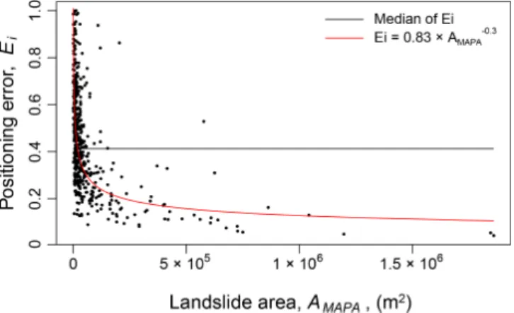
We identified 482 pairs of corresponding landslides for which we calculated the positioning error Ei, with values in the range of 0.05 to 1.00. The average value for the po-sitioning errorEi was 0.44, and the median of the error was 0.41 (dashed line in Fig. 10). We compare these figures to the mapping error E=0.19, computed using the method pro-posed by Carrara et al. (1992). In Fig. 10, for each pair of corresponding landslides, we plot the value ofEi against the area AL of the landslide shown in map A (produced using the manual method). Inspection of the plot reveals that the positioning error Ei is largest for the very small landslides and (with a few exceptions) decreases rapidly with increas-ing landslide area. For slope failures withAL<1×10⁵m2, the positioning errorEiexhibits a large variability. For land-slides withAL>1×10⁵m2the positioning errorEiis gen-erally smaller than 0.3, and does not exceed 0.1 for landslides withAL>4.2×10⁵m2.
Figure 10 shows that large positioning errors are associ-ated to small landslides. When analysing stereoscopic APs visually, small landslides are identified based primarily on their photographic evidence (tone, mottling, pattern, texture) in the photographs, and not based on their morphological characteristics (the presence, association, and pattern of e.g. concavities, convexities, escarpments, back-slopes), which can be very subtle. However, this photographic information is typically not shown in the topographic maps, making it difficult for the interpreter to locate and map the small
land-Figure 10. Scatter plot of the positioning error index (Ei) against the landslide area, mapped using the traditional procedure (AMAPA). The plot shows a heavy-tailed distribution of Ei that decays with increasing landslide area, following a power-law (red line). Both axes are in linear scale. The median value ofEi (0.41) is displayed by a black line.
slides in the base map accurately. In other words, when the interpreter transfers small landslides from the AP to the base map visually, he/she uses a subset of the information avail-able for the detection of the landslide in the AP. Lack of in-formation contributed to the mapping error. Conversely, large landslides typically exhibit a distinct morphological signa-ture (Pike, 1988) that is shown (partially or totally) in the topographic maps, making it simpler for the interpreter to transfer the landslide information to the base map accurately. This reduces the mapping error for large and very large land-slides. The same applies to channelled debris flows that occur primarily along channels visible on the topographic maps, and deposit the failed material on debris fans that are also visible on the topographic maps.
5 Discussion
We tested a new semi-automatic procedure to transfer landslide and other geomorphological information captured through API from the original aerial photographs to a digi-tal landslide database in a GIS environment. The new pro-cedure can contribute to the efficient production of accurate LIMs and geomorphological maps over large areas. Consid-ering the entire landslide mapping process exemplified in Fig. 2, the semi-automatic procedure reduces significantly (or avoids completely) the subjectivity introduced by the vi-sual (manual) transfer of the landslide and geomorpholog-ical information from the APs to the digital database. This reduces mapping errors, enhancing the quality of a LIM.
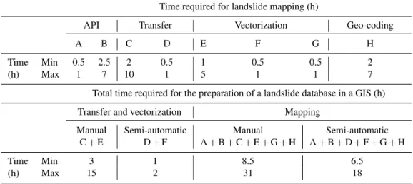
API Transfer Vectorization Geo-coding
A B C D E F G H
Time Min 0.5 2.5 2 0.5 1 0.5 0.5 2
(h) Max 1 7 10 1 5 1 1 7
Total time required for the preparation of a landslide database in a GIS (h)
Transfer and vectorization Mapping
Manual Semi-automatic Manual Semi-automatic
C+E D+F A+B+C+E+G+H A+B+D+F+G+H
Time Min 3 1 8.5 6.5
(h) Max 15 2 31 18
not available to us (as is rarely the case in landslide map-ping, Santangelo et al., 2010), and being aware of the RMSE of 7.7 m introduced by the orthorectification of the APs in map B (C2 in Fig. 2), we consider map B as reasonably “cor-rect” in terms of the geographical location, size, and shape of the mapped landslides. As a consequence, we interpret the observed differences (mismatches) in map A as errors intro-duced by the visual transfer of the landslide information in the manual procedure (C1 in Fig. 2).
We measured the overall degree of mismatching between the two inventories (map A vs. map B) using the error index E (Eq. 1) introduced by Carrara et al. (1992), and obtained a value for the mapping error indexE=0.19. This suggests that overall, the two maps are rather similar (Ardizzone et al., 2002). Visual inspection of Fig. 7 confirms the impression. However, inspection of Fig. 8 reveals a number of (small and large) local differences between single landslide pairs in the two inventories. To quantify the individual differences, we calculated the positional errorEifor 482 pairs of correspond-ing landslides in the two inventories. The result revealed po-sitional errors in the range 0.05≤Ei≤1.00, with an aver-age errorEi=0.44. The difference withE=0.19 is signif-icant, and suggests that the lumped measure provided by the mapping error indexEof Carrara et al. (1992) overestimates the degree of geographical matching (and underestimates the mismatch) between the two maps.
Our results also revealed that the positional error of sin-gle landslidesEi depends on the sizeAL of the landslides, with small landslides exhibiting a larger positional error than larger landslides (Fig. 10). Interestingly, the dependence of the positional error on landslide area is well approximated by a power-law,Ei=8.03×A−L0.3. This information can be used to estimate the expected positional error of single
land-slides in LIMs produced manually. We maintain that this is important (and new) information for the users of a LIM.
Time is a critical aspect in the production of LIMs. For a LIM covering a large or very large area (thousands of square kilometres) the production of an accurate inventory map can take several months to a few years (Galli et al., 2008; Guzzetti et al., 2012). A significant part of the time used to prepare a LIM is spent in transferring the landslide informa-tion from the APs to the digital landslide database. The new semi-automatic procedure reduces the time (and hence the cost) for the production of a LIM significantly.
(and fast) in urban areas, and difficult (and time-consuming) in rural or forested areas where adequate GCPs were difficult to identify. The time required for all geo-coding operations depended on the quantity of the landslides and the other geo-morphological features, and on their geographical and topo-logical relationships.
Comparison of the time required for transferring the land-slide information from the APs to the GIS database (without geo-coding) reveals that the new procedure (and specifically the orthorectification step) accelerated the process by a fac-tor of 4–10, compared to the visual (manual) transfer. If geo-coding is considered, the acceleration factor is in the range of 3 to 8 (Table 3). The improvement is significant, and mea-sures the gain in efficiency introduced by the semi-automatic procedure. When the entire mapping workflow is considered (Fig. 2) the gain in efficiency is somewhat lower, but remains significant. The difference (gain) in time for one person to complete the mapping of one stereogram ranged from a min-imum of 2 h to a maxmin-imum of 13 h. These figures suggest that the new semi-automatic procedure is always more convenient (more efficient) than the traditional (manual) procedure, with the efficiency increasing where the geomorphological com-plexity of the area increases.
In our experiment, the API phase took a total of 31.5 h. Orthorectification of the APs took 4.5 h. This compares to 35 h required for the visual transfer of the information with the manual procedure. Automatic vectorization took 4.5 h, which compares to the 22 h for the manual vectorization. Geo-coding required the same amount of time for both cedures (32 h). Overall, using the new semi-automatic pro-cedure the time needed to complete the landslide inventory (map B) was 40.5 h, which is 44 % of the time (92.5 h) used to prepare the inventory adopting the traditional mapping pro-cedure (map A). Including the API phase, the time used to cover an area of 93 km2with a detailed (1 : 10 000 scale) ge-omorphological LIM (Guzzetti et al., 2012) was 72 h (nine working days) using the semi-automatic procedure, and was 124 h (15.5 working days) using the manual procedure. In other words, the new procedure increased the interpreter’s productivity from 0.32 to 0.55 stereograms per person per day, a 72 % increase. For completing the landslide mapping of one stereogram, a geomorphologist needs 2 days using the new semi-automatic procedure, and 3 days using the tradi-tional manual procedure. We acknowledge that these figures are estimates, and subjected to variations depending on the local geological, morphological and land use settings, on the quality of the topographic base map, on the number and com-plexity of the landslides and on their geometrical and topo-logical relationships.
Despite the clear gain in mapping accuracy and efficiency, the new semi-automatic procedure is not free of problems, and care is needed when using the procedure to prepare a LIM. A number of factors influence the geographical accu-racy of the landslides shown in a LIM produced by carrying out the semi-automatic procedure, including the accuracy of
the DEM, of the interior orientation, and of the GCPs used for the exterior orientation. Selection of the GCPs for the ex-terior orientation is a crucial, and the most delicate step of the procedure. Accuracy of this step depends on the geographical accuracy and resolution of the base map, and on the differ-ence in age between the base map and the aerial photographs that need to be orthorectified. In our study, the aerial pho-tographs were taken in 2005, and the orthophotograph (base map) used to select the GCPs was taken in 2007 with a res-olution of 0.25 m. This made it simple to identify the GCPs accurately. In other areas, accurate selection of a sufficient number of GCPs may be problematic, limiting the quality of the orthorectified image.
Figure 6 shows that the geographical co-registration be-tween the orthorectified aerial photographs and the orthopho-tograph (base map) used for the exterior orientation is not perfect, and that it is slightly worse along the N–S direction than along the E–W direction. When a LIM is shown on a base map different from the map used for the orthorectifi-cation, the differences (including co-registration errors) be-tween the two base maps combine, contributing to degrad-ing the location accuracy of the landslides shown in the new base map. In our study, the co-registration accuracy plots portrayed in Fig. 6a and b show that 95 % of the overall co-registration errors are within a range of 9.0 m along the xaxis (E–W direction), and 10.1 m along theyaxis (N–S di-rection). The sum of the total RMSEs for the two base maps (i.e. the RMSE obtained between the orthorectified APs and the orthophotograph, and the RMSE obtained between the orthophotograph and the topographic map) is 7.7 m. We con-sider this is an acceptable error for a 1 : 10 000 scale LIM (∼0.8 mm on the map).
lations depend on the accuracy of the multi-temporal or sea-sonal maps. Misplaced landslides can result in an overesti-mation or underestioveresti-mation of the temporal frequency of land-slides in an area (Fig. 7c), introducing errors affecting haz-ard and risk assessments, and erosion studies. Landslide po-sitioning errors can have serious impacts on the definition of vulnerable elements, leading to locally erroneous estimations of landslide risk. Our results suggest that geographically ac-curate LIMs prepared by adopting the semi-automatic proce-dure should be preferred to construct accurate multi-temporal or seasonal inventories.
LIMs are also used to determine the statistics of landslide size (area and volume) (Malamud et al., 2004a; Guzzetti et al., 2009), and to investigate correlations between the loca-tion and abundance of landslides and the local geological structure (Grelle et al., 2011; Marchesini et al., 2013; Santan-gelo et al., 2015b). Our results revealed that the geographical accuracy of the location (and hence the shape and size) of the landslides depends on the size of the slope failures (Fig. 7c), with larger positional errors expected for small landslides than for large landslides. The positional errors affecting the small landslides may result in biases in the size of the small failures. This may affect the determination of accurate statis-tics of landslide areas, and particularly the definition of the most common size for the landslides in a study area i.e., the “rollover” size (Stark and Hovius, 2001; Guzzetti et al., 2002; Malamud et al., 2004b, Stark and Guzzetti, 2009). On the other hand, statistics of the total (cumulated) landslide area and volume, being controlled by the few largest land-slides in an inventory (Guzzetti et al., 2008), are not expected to be biased by the positioning errors inevitably present in the inventories, which our results suggest are reduced for very large landslides (Fig. 10).
Guzzetti et al. (2012) and Jackson et al. (2012) have pointed out the need for standards for the production of LIMs. Lack of standards remains a problem that limits the credibility and usefulness of LIMs. The results of our work confirm that standards for transferring the information from the APs to a digital landslide map can (and should) be es-tablished. We argue that LIMs produced through API should be accompanied by adequate information (metadata) to ex-plain clearly and unambiguously (among other things) how the landslide information was transferred from the APs to the GIS landslide database. For LIMs produced though a visual transfer of the information (e.g. our map A), the power-law dependency shown in Fig. 10 (or similar relationships) can be used to quantify (and show) the expected positional er-rors for the landslides shown in the inventory. For maps pro-duced through a robust orthorectification procedure (e.g. our
will be suited also to the production of thematic maps (e.g. land-use maps or morpho-structural maps) based on informa-tion obtained from the interpretainforma-tion of APs.
6 Conclusions
Preparing accurate landslide inventory maps (LIMs) is cru-cial to modern landslide research. However, the production of accurate LIMs is time-consuming, limiting the ability of investigators to cover large areas. Also, the production of LIMs remains a largely manual (craftsmanship) exercise. This introduces subjectivity and errors in the process, and increases the costs for the production of the LIMs.
We have experimented a new procedure for the semi-automatic mapping of landslides that uses robust orthorec-tification in a GIS environment to transfer accurately and ef-ficiently landslide information drawn by an interpreter on the aerial photographs into a digital landslide database stored in the GIS. The new semi-automatic procedure reduces the time and effort required to prepare a LIM significantly, augment-ing the interpreter’s efficiency and productivity by a factor of∼2. The semi-automatic procedure results in the produc-tion of more accurate LIMs, compared to landslide maps pro-duced manually.
Systematic application of the new procedure in a 93 km2 area in NE Sicily, Italy, revealed that a common metric used to evaluate the degree of matching (or mismatching) between two LIMs available for the same area (Carrara et al., 1992; Ardizzone et al., 2002) underestimates (severely, in places) the local mismatch between pairs of corresponding land-slides in the two inventories. Our results further revealed a dependency of the positional error of a landslide on the size of the landslide, with small landslides characterized by sig-nificantly larger errors than the large and very large land-slides. The finding has potential consequences for multiple applications of landslide studies.
Acknowledgements. We thank Mauro Rossi, CNR IRPI, for determining the probability distribution of landslide areas for the two inventories. M. Santangelo, F. Bucci, were partially supported by a grant of the Italian National Department of Civil Protection. F. Fiorucci was supported by a grant of the Umbria Region, under contract POR-FESR 861,2012. This research was conducted during M. Santangelo PhD studies at Dipartimento di Fisica e Geologia, Università degli Studi di Perugia, Piazza dell’Università 1, 06100 Perugia, Italy.
Disclaimer.In this work, use of copyright, brand, trade names, and logos is for descriptive and identification purposes only, and does not imply endorsement from the authors, or their institutions.
Edited by: K.-T. Chang
Reviewed by: P. Bobrowsky and one anonymous referee
References
Antonini, G., Cardinali, M., Guzzetti, F., Reichenbach, P., and Sor-rentino, A.: Carta Inventario dei Fenomeni Franosi della Regione Marche ed aree limitrofe, Publication no. 580, 2 sheets, 2816, 2817, 2836, scale 1 : 100 000, CNR Gruppo Nazionale per la Difesa dalle Catastrofi Idrogeologiche, Rome, 1993.
Antonini, G., Ardizzone, F., Cacciano, M., Cardinali, M., Castel-lani, M., Galli, M., Guzzetti, F., Reichenbach, P., and Sal-vati, P.: Rapporto Conclusivo Protocollo d’Intesa fra la Regione dell’Umbria, Direzione Politiche Territoriali Ambiente e Infras-trutture, ed il CNR IRPI di Perugia per l’acquisizione di nuove informazioni sui fenomeni franosi nella regione dell’Umbria, la realizzazione di una nuova carta inventario dei movimenti fra-nosi e dei siti colpiti da dissesto, l’individuazione e la perime-trazione delle aree a rischio da frana di particolare rilevanza, e l’aggiornamento delle stime sull’incidenza dei fenomeni di dissesto sul tessuto insediativo, infrastrutturale e produttivo re-gionale, Unpublished report, May 2002, 140 pp., 2002a. Antonini, G., Ardizzone, F., Cardinali, M., Galli, M., Guzzetti, F.,
and Reichenbach, P.: Surface deposits and landslide inventory map of the area affected by the 1997 Umbria-Mare earthquakes, B. Soc. Geol. Ital., 121, 843–853, 2002b.
APAT: Servizio Geologico d’Italia, Dipartimento Difesa del Suolo, Carta Geologica d’Italia alla scala 1 : 50 000, Foglio 613 Taormina, S.EL.CA., Firenze, available at: http://www. isprambiente.gov.it/Media/carg/613_TAORMINA/Foglio.html (last access: 30 June 2015), 2008.
Ardizzone, F., Cardinali, M., Carrara, A., Guzzetti, F., and Re-ichenbach, P.: Impact of mapping errors on the reliability of landslide hazard maps, Nat. Hazards Earth Syst. Sci., 2, 3–14, doi:10.5194/nhess-2-3-2002, 2002.
Ardizzone, F., Cardinali, M., Galli, M., Guzzetti, F., and Reichen-bach, P.: Identification and mapping of recent rainfall-induced landslides using elevation data collected by airborne Lidar, Nat. Hazards Earth Syst. Sci., 7, 637–650, doi:10.5194/nhess-7-637-2007, 2007.
Ardizzone, F., Basile, G., Cardinali, M., Casagli, N., Del Conte, S., Del Ventisette, C., Fiorucci, F., Garfagnoli, F., Gigli, G., Guzzetti, F., Iovine, G. G. R., Mondini, A. C., Moretti, S., Panebianco, M., Raspini, F., Reichenbach, P., Rossi, M.,
Tan-teri, L., and Terranova, O. G.: Landslide inventory map for the Briga and the Giampilieri catchments, NE Sicily, Italy, J. Maps, 8, 176–180, doi:10.1080/17445647.2012.694271, 2012. Ardizzone, F., Fiorucci, F., Santangelo, M., Cardinali, M.,
Mon-dini, A. C., Rossi, M., Reichenbach, P., and Guzzetti, F.: Use of very-high resolution stereoscopic satellite images for landslide mapping, in: Landslide Science and Practice, edited by: Margot-tini, C., Canuti, P., and Sassa, K., Springer, Berlin, Heidelberg, 95–101, 2013.
Bernstein, R.: Image geometry and rectification, in: Manual of Re-mote Sensing, edited by: Colwell, R. N., American Society of Photogrammetry, Falls Church, VA, 1983.
Borghuis, A. M., Chang, K., and Lee, H. Y.: Comparison between automated and manual mapping of typhoon-triggered landslides from SPOT-5 imagery, Int. J. Remote Sens., 28, 1843–1856, 2007.
Brabb, E. E. and Pampeyan, E. H.: Preliminary map of landslide deposits in San Mateo County, California, US Geological Sur-vey Miscellaneous Field Studies Map, MF-344, US Geological Survey, 1972.
Brabb, E. E., Wieczorek, G. F., and Harp, E. L.: Map showing 1983 landslides in Utah, U.S. Geological Survey Miscellaneous Field Studies Map, MF-1867, US Geological Survey, 1989.
Brunsden, D.: Mass movements; the research frontier and beyond: a geomorphological approach, Geomorphology, 7, 85–128, 1993. Cardinali, M., Guzzetti, F., and Brabb, E. E.: Preliminary map
showing landslide deposits and related features in New Mexico, US Geological Survey Open File Report 90/293, 4 sheets, scale 1 : 500 000, US Geological Survey, Washington, 1990.
Cardinali, M., Antonini, G., Reichenbach, P., and Guzzetti, F.: Photo geological and landslide inventory map for the Upper Tiber River basin, Publication n. 2116, scale 1 : 100 000, GNDCI INternal Report, CNR, Gruppo Nazionale per la Difesa dalle Catastrofi Idrogeologiche, Rome, 2001.
Cardinali, M., Reichenbach, P., Guzzetti, F., Ardizzone, F., An-tonini, G., Galli, M., Cacciano, M., Castellani, M., and Sal-vati, P.: A geomorphological approach to the estimation of land-slide hazards and risks in Umbria, Central Italy, Nat. Hazards Earth Syst. Sci., 2, 57–72, doi:10.5194/nhess-2-57-2002, 2002. Carrara, A., Cardinali, M., and Guzzetti, F.: Uncertainty in assessing
landslide hazard and risk, ITC Journal, 2, 172–183, 1992. Cheng, K. S., Wei, C., and Chang, S. C.: Locating landslides using
multi-temporal satellite images, Adv. Space Res., 33, 96–301, 2004.
Congalton, R. G.: A review of assessing the accuracy of classifica-tions of remotely sensed data, Remote Sens. Environ., 37, 35–46, 1991.
Cruden, D. M. and Varnes, D. J.: Landslide types and processes, in: Landslides, Investigation and Mitigation, edited by: Turner, A. K. and Schuster, R. L., Transportation Research Board Special Re-port 247, Washington, D.C., 36–75, 1996.
Delaunay, J.: Carte de France des zones vulnèrables a des glisse-ments, écrouleglisse-ments, affaissements et effrondrements de ter-rain, 81 SGN 567 GEG, Bureau de Recherches Géologiques et Minières, 23 pp., 1981.
Di Maggio, C., Madonia, G., and Vattano, M.: Deep-seated gravitational slope deformations in western Sicily:
morpho-slides mapping and estimation of landslide mobilization rates using aerial and satellite images, Geomorphology, 129, 59–70, doi:10.1016/j.geomorph.2011.01.013, 2011.
Galli, M., Ardizzone, F., Cardinali, M., Guzzetti, F., and Reichen-bach, P.: Comparing landslide inventory maps, Geomorphology, 94, 268–289, doi:10.1016/j.geomorph.2006.09.023, 2008. Gao, J. and Maroa, J.: Topographic controls on
evolu-tion of shallow landslides in pastoral Wairarapa, New
Zealand, 1979–2003, Geomorphology, 114, 373–381,
doi:10.1016/j.geomorph.2009.08.002, 2010.
Giordan, D., Allasia, P., Manconi, A., Baldo, M., Santangelo, M., Cardinali, M., Corazza, A., Albanese, V., Lollino, G., and Guzzetti, F.: Morphological and kinematic evolution of a large earthflow: the Montaguto landslide, southern Italy, Geomorphol-ogy, 187, 61–79, 2013.
GRASS Development Team: Geographic Resources Analysis Sup-port System (GRASS) Software, Version 6.4.0, Open Source Geospatial Foundation, available at: http://grass.osgeo.org (last access: 30 June 2015), 2012.
Grelle, G., Revellino, P., Donnarumma, A., and Guadagno, F. M.: Bedding control on landslides: a methodological approach for computer-aided mapping analysis, Nat. Hazards Earth Syst. Sci., 11, 1395–1409, doi:10.5194/nhess-11-1395-2011, 2011. Guzzetti, F. and Cardinali, M.: Carta Inventario dei Fenomeni
Fra-nosi della Regione dell’Umbria ed aree limitrofe, Publication n. 204, 2 sheets, scale 1 : 100 000, CNR, Gruppo Nazionale per la Difesa dalle Catastrofi Idrogeologiche, Rome, 1989.
Guzzetti, F. and Cardinali, M.: Landslide inventory map of the Um-bria region, Central Italy, in: Proceedings ALPS 90 6th Interna-tional Conference and Field Workshop on Landslides, edited by: Cancelli, A., Milan, Italy, 273–284, 1990.
Guzzetti, F., Malamud, B. D., Turcotte, D. L., and Reichenbach, P.: Power-law correlations of landslide areas in central Italy, Earth Planet. Sc. Lett., 195, 169–183, 2002.
Guzzetti, F., Reichenbach, P., Cardinali, M., Galli, M., and Ardizzone, F.: Probabilistic landslide hazard assess-ment at the basin scale, Geomorphology, 72, 272–299, doi:10.1016/j.geomorph.2005.06.002, 2005.
Guzzetti, F., Galli, M., Reichenbach, P., Ardizzone, F., and Cardi-nali, M.: Landslide hazard assessment in the Collazzone area, Umbria, Central Italy, Nat. Hazards Earth Syst. Sci., 6, 115–131, doi:10.5194/nhess-6-115-2006, 2006.
Guzzetti, F., Ardizzone, F., Cardinali, M., Galli, M., and Re-ichenbach, P.: Distribution of landslides in the Upper Tiber River basin, central Italy, Geomorphology, 96, 105–122, doi:10.1016/j.geomorph.2007.07.015, 2008.
Guzzetti, F., Ardizzone, F., Cardinali, M., Rossi, M., and Valigi, D.: Landslide volumes and landslide mobilization rates in Um-bria, central Italy, Earth Planet. Sc. Lett., 279, 222–229, doi:10.1016/j.epsl.2009.01.005, 2009.
Guzzetti, F., Mondini, A. C., Cardinali, M., Fiorucci, F., San-tangelo, M., and Chang, K. T.: Landslide inventory maps:
tion, Maps and Mapping – Canadian Technical Guidelines and Best Practices Related to Landslides: A National Initiative for Loss Reduction, Geological Survey of Canada, Open File 7059, doi:10.4095/292122, 2012.
Lu, P., Stumpf, A., Kerle, N., and Casagli, N.: Object-oriented change detection for landslide rapid mapping, IEEE T. Geosci. Remote, 8, 701–705, 2011.
Malamud, B. D., Turcotte, D. L., Guzzetti, F., and Reichenbach, P.: Landslide inventories and their statistical properties, Earth Surf. Proc. Land., 29, 687–711, 2004a.
Malamud, B. D., Turcotte, D. L., Guzzetti, F., and Reichenbach, P.: Landslides, earthquakes, and erosion, Earth Planet. Sci. Lett., 229, 45–59, doi:10.1016/j.epsl.2004.10.018, 2004b.
Marcelino, E. V., Formaggio, A. R., and Maeda, E. E.: Landslide inventory using image fusion techniques in Brazil, Int. J. Appl. Earth Obs., 11, 181–191, 2009.
Marchesini, I., Santangelo, M., Fiorucci, F., Cardinali, M., Rossi, M., and Guzzetti, F.: A GIS method for obtaining geo-logic bedding attitude, in: Landslide Science and Practice, edited by: Margottini, C., Canuti, P., and Sassa, K., Springer, Berlin, Heidelberg, 243–247, 2013.
Martha, T. R., Kerle, N., Jetten, V., van Westen, C., and Vinod Ku-mar, K.: Characterising spectral, spatial and morphometric prop-erties of landslides for semi-automatic detection using object-oriented methods, Geomorphology, 116, 24–36, 2010.
McDonald, H. C. and Grubbs, R. C.: Landsat imagery analysis: an aid for predicting landslide prone areas for highway construction, Vol. 1-b, NASA Earth Resource Survey Sym., Houston, Texas, 769–778, 1975.
Mondini, A. C. and Chang, K.-T.: Combining spectral and
geoenvironmental information for probabilistic event
landslide mapping, Geomorphology, 213, 183–189,
doi:10.1016/j.geomorph.2014.01.007, 2014.
Mondini, A. C., Chang, K.-T., and Yin, H.-Y.: Combin-ing multiple change detection indices for mappCombin-ing land-slides triggered by typhoons, Geomorphology, 134, 440–451, doi:10.1016/j.geomorph.2011.07.021, 2011a.
Mondini, A. C., Guzzetti, F., Reichenbach, P., Rossi, M., Cardi-nali, M., and Ardizzone, F.: Semi-automatic recognition and mapping of rainfall induced shallow landslides using satel-lite optical images, Remote Sens. Environ., 115, 1743–1757, doi:10.1016/j.rse.2011.03.006, 2011b.
Mondini, A. C., Marchesini, I., Rossi, M., Chang, K.-T., Pasquar-iello, G., and Guzzetti, F.: Bayesian framework for map-ping and classifying shallow landslides exploiting remote sens-ing and topographic data, Geomorphology, 201, 135–147, doi:10.1016/j.geomorph.2013.06.015, 2013.
Murillo-García, F. G., Alcántara-Ayala, I., Ardizzone, F., Cardi-nali, M., Fiourucci, F., and Guzzetti, F.: Satellite stereoscopic pair images of very high resolution: a step forward for the de-velopment of landslide inventories, Landslides, 12, 277–291, doi:10.1007/s10346-014-0473-1, 2015.
Nichol, E. J., Shaker, A., and Wong, M. S: Application of high-resolution stereo satellite images to detailed landslide hazard as-sessment, Geomorphology, 76, 68–75, 2006.
Pike, R. J.: The geometric signature: quantifying landslide-terrain types from digital elevation models, Math. Geol., 20, 491–511, doi:10.1007/BF00890333, 1988.
Radbruch-Hall, D. H., Colton, R. B., Davies, W. E., Lucchitta, I., Skipp, B. A., and Varnes, D. J.: Landslide overview map of the conterminous United States, US Geological Survey Professional Paper 1183, US Geological Survey, Washington, 25 pp., 1982. Razak, K. A., Straatsma, M. W., van Westen, C. J., Malet,
J.-P., and de Jong, S. M.: Airborne laser scanning of forested landslides characterization: terrain model
qual-ity and visualization, Geomorphology, 126, 186–200,
doi:10.1016/j.geomorph.2010.11.003, 2011.
Razak, K. A., Santangelo, M., Van Westen, C. J., Straatsma, M. W., and de Jong, S. M.: Generating an optimal DTM from airborne laser scanning data for landslide mapping in a tropical forest en-vironment, Geomorphology, 190, 112–125, 2013.
Reichenbach, P., Guzzetti, F., and Cardinali., M.: Map of sites his-torically affected by landslides and floods, The AVI Project, 2nd Edn., CNR GNDCI Publication Number 1782, map at 1 : 1 200 000 scale, CNR, Rome, 1998.
Reichenbach, P., Galli, M., Cardinali, M., Guzzetti, F., and Ardiz-zone, F.: Geomorphological mapping to assess landslide risk: concepts, methods and applications in the Umbria region 25 of Central Italy, in: Landslide Hazard and Risk, edited by: Glade, T., Anderson, M. G., and Crozier, M. J., John Wiley & Sons, Ltd., Chippenham, 429–468, 2004.
Rocchini, D., Metz, M., Frigeri, A., Delucchi, L., Marcantonio, M., and Neteler, M.: Robust rectification of aerial photographs in an open source environment, Computers Geosci., 39, 145–151, doi:10.1016/j.cageo.2011.06.002, 2011.
Rosin, P. L. and Hervás, J.: Remote sensing image thresholding methods for determining landslide activity, Int. J. Remote Sens., 26, 1075–1092, 2005.
Rossi, M., Guzzetti, F., Reichenbach, P., Mondini, A. C., and Peruccacci, S.: Optimal landslide susceptibility zonation based on multiple forecasts, Geomorphology, 114, 129–142, doi:10.1016/j.geomorph.2009.06.020, 2009.
Salvati, P., Guzzetti, F., Reichenbach, P., Cardinali, M., and Stark, C. P.: Map of landslides and floods with human con-sequences in Italy, CNR Gruppo Nazionale per la Difesa dalle Catastrofi Idrogeologiche Publication n. 2822, scale 1 : 1 200 000, CNR, Rome, 2003.
Santangelo, M., Cardinali, M., Rossi, M., Mondini, A. C., and Guzzetti, F.: Remote landslide mapping using a laser rangefinder binocular and GPS, Nat. Hazards Earth Syst. Sci., 10, 2539– 2546, doi:10.5194/nhess-10-2539-2010, 2010.
Santangelo, M., Maresini, I., Bucci, F., Fiorucci, F., Cardinali, M., and Guzzetti, F.: Landslide mapping: improving accuracy and ef-ficiency, in: Proceedings of the 7th EUREGEO Congress, 12– 15 June 2012, Bologna, 788–789, 2012.
Santangelo, M., Gioia, D., Cardinali, M., Guzzetti, F., and Schiattarella, M.: Interplay between mass move-ment and fluvial network organization: an example from southern Apennines, Italy, Geomorphology, 188, 54–67, doi:10.1016/j.geomorph.2012.12.008, 2013.
Santangelo, M., Gioia, D., Cardinali, M., Guzzetti, F., and Schiattarella, M.: Landslide inventory map for the upper Sinni River valley, Southern Italy, J. Maps, 11, 444–453, doi:10.1080/17445647.2014.949313, 2015a.
Santangelo, M., Marchesini, I., Cardinali, M., Fiorucci, F., Rossi, M., Bucci, F., and Guzzetti, F.: A method for the assessment of the influence of bedding on landslide abundance and types, Land-slides, 12, 295–309, doi:10.1007/s10346-014-0485-x, 2015b. Sauchyn, D. J. and Trench, N. R.: Landsat applied to landslide
map-ping, Photogramm. Eng. Rem. S., 44, 735–741, 1978.
Stark, C. P. and Guzzetti, F.: Landslide rupture and the probability distribution of mobilized debris volumes, J. Geophys. Res., 114, F00A02, doi:10.1029/2008JF001008, 2009.
Stark, C. P. and Hovius, N.: The characterization of land-slide size distributions, Geophys. Res. Lett., 28, 1091–1094, doi:10.1029/2000GL008527, 2001.
Stumpf, A. and Kerle, N.: Object-oriented mapping of landslides using Random Forest, Remote Sens. Environ., 115, 2564–2577, doi:10.1016/j.rse.2011.05.013, 2011.
Thiery, Y., Malet, J.-P., Sterlacchini, S., Puissant, A., and Maquaire, O.: Landslide susceptibility assessment by bivariate methods at large scales: application to a complex mountainous environment, Geomorphology, 92, 38–59, 2007.
Trigila, A., Iadanza, C., and Spizzichino, D.: Quality assessment of the Italian Landslide Inventory using GIS processing, Land-slides, 7, 455–470, doi:10.1007/s10346-010-0213-0, 2010. Van Den Eeckhaut, M., Poesen, J., Verstraeten, G., Vanacker, V.,
Moeyersons, J., Nyssen, J., van Beek, L. P. H., and Vandek-erckhove, L.: Use of LIDAR-derived images for mapping old landslides under forest, Earth Surf. Proc. Land., 32, 754–769, doi:10.1002/esp.1417, 2007.
Van Den Eeckhaut, M., Kerle, N., Poesen, J., and Hervás, J.: Object-oriented identification of forested landslides with derivatives of single pulse LiDAR data. Geomorphology, 173–174, 30–42, doi:10.1016/j.geomorph.2012.05.024, 2012.