COMPARISON BETWEEN DETAILED DIGITAL AND CONVENTIONAL SOIL MAPS OF AN AREA WITH COMPLEX GEOLOGY

COMPARISON BETWEEN DETAILED DIGITAL AND

CONVENTIONAL SOIL MAPS OF AN AREA WITH COMPLEX

GEOLOGY

Osmar Bazaglia Filho(2), Rodnei Rizzo(3), Igo Fernando Lepsch(4), Hélio do Prado(5), Felipe Haenel Gomes(6), Jairo Antonio Mazza(7) & José Alexandre Melo Demattê(7)

SUMMARY

Since different pedologists will draw different soil maps of a same area, it is important to compare the differences between mapping by specialists and mapping techniques, as for example currently intensively discussed Digital Soil Mapping. Four detailed soil maps (scale 1:10.000) of a 182-ha sugarcane farm in the county of Rafard, São Paulo State, Brazil, were compared. The area has a large variation of soil formation factors. The maps were drawn independently by four soil scientists and compared with a fifth map obtained by a digital soil mapping technique. All pedologists were given the same set of information. As many field expeditions and soil pits as required by each surveyor were provided to define the mapping units (MUs). For the Digital Soil Map (DSM), spectral data were extracted from Landsat 5 Thematic Mapper (TM) imagery as well as six terrain attributes from the topographic map of the area. These data were summarized by principal component analysis to generate the map designs of groups through Fuzzy K-means clustering. Field observations were made to identify the soils in the MUs and classify them according to the Brazilian Soil Classification System (BSCS). To compare the conventional and digital (DSM) soil maps, they were crossed pairwise to generate confusion matrices that were mapped. The categorical analysis at each classification level of the BSCS showed that the agreement between the maps

(1) _{Part of the Dissertation of the first author, submitted to the Escola Superior de Agricultura "Luiz de Queiroz" - ESALQ/USP.}

Received for publication on November 1st, 2012 and approved on July 11, 2013.

(2) _{Agronomist MSc. Usina São José da Estiva S/A - Açúcar e Álcool. Fazenda Três Pontes. Caixa Postal 121. CEP 14960-000 Novo}

Horizonte (SP). Grand holder of CAPES no período de 02/2010-02/2012. E-mail: osmarbazaglia@gmail.com

(3) _{Agronomist MSc. ESALQ/USP. E-mail: rodnei.rizzo@gmail.com}

(4) _{Visiting Researcher, Department of Soil Science and Plant Nutrition (DCS) - ESALQ/USP. Av. Pádua Dias, 11. CEP 13418-000}

Piracicaba (SP). E-mail: igo.lepsch@yahoo.com.br

(5) _{Researcher, Instituto Agronômico de Campinas - IAC/APTA - Centro Cana-de-açúcar. Rod. Antonio Duarte Nogueira, km 321.}

CEP 14001-970 Ribeirão Preto (SP). E-mail: heprado@terra.com.br

(6) _{PhD, DCS - ESALQ/USP. E-mail: felipehgomes@yahoo.com.br}

decreased towards the lower levels of classification and the great influence of the surveyor on both the mapping and definition of MUs in the soil map. The average correspondence between the conventional and DSM maps was similar. Therefore, the method used to obtain the DSM yielded similar results to those obtained by the conventional technique, while providing additional information about the landscape of each soil, useful for applications in future surveys of similar areas.

Index terms: soil cartography, detailed soil survey, remote sensing, soil-landscape relationship.

RESUMO: COMPARAÇÃO ENTRE MAPAS DE SOLOS DETALHADOS

OBTIDOS PELOS MÉTODOS CONVENCIONAL E DIGITAL EM UMA ÁREA DE GEOLOGIA COMPLEXA

Uma vez que pedólogos diferentes produzirão, em uma mesma área, mapas de solos distintos, é importante avaliar as divergências existentes entre profissionais e técnicas de mapeamento, dentre elas o Mapeamento Digital de Solos, que vem sendo muito abordada atualmente. Para tanto, compararam-se quatro mapas detalhados de solos (escala 1:10.000) de uma fazenda de 182 ha cultivados com cana-de-açúcar, localizada no município de Rafard, SP, com grande variação do meio físico. Tais mapas foram elaborados independentemente por quatro pedólogos e confrontados com outro obtido com o apoio de uma técnica de mapeamento digital de solos. Aos pedólogos, foram fornecidas mesmas informações; cada um foi levado ao campo o número de vezes que julgou necessário para examinar os solos (paisagem e perfis), delinear as unidades de mapeamento (UM) e indicar os locais onde desejava examinar o perfil do solo e, ou, amostrá-lo para análises laboratoriais. Para o MDS, foram utilizados dados espectrais de uma imagem do sensor TM do satélite Landsat 5 e seis atributos de terreno derivados de carta planialtimétrica. Essas informações foram resumidas por análise de componentes principais e utilizadas para geração dos delineamentos em um mapa de grupos, com auxílio da análise de grupamentos Fuzzy K-médias. Posteriormente, em cada delineamento, foram feitas observações de campo para identificar os solos componentes das UMs, de acordo com o Sistema Brasileiro de Classificação de Solos (SiBCS). Para comparações entre os mapas convencionais e entre esses e o mapa digital de solos (MDS), efetuaram-se cruzamentos entre os mapas dois a dois, gerando matrizes de confusão, apresentadas na forma de mapas. A análise das correspondências espaciais, para cada nível categórico do SiBCS, permitiu verificar que a concordância entre a correspondência na identificação das UMs nos mapas decresce para os níveis categóricos inferiores e que o executor exerce grande influência nos delineamentos e na identificação das UMs do mapa de solos. A correspondência espacial média entre mapas convencionais e entre esses e o MDS foram semelhantes. Portanto, o método utilizado para obter esse MDS proporcionou resultados similares aos obtidos com os mapas convencionais, com as vantagens de quantificar informações sobre as características da paisagem de cada solo, úteis para extrapolar resultados para futuros levantamentos que forem efetuados em áreas com solos similares.

Termos de indexação: cartografia de solos, levantamento pedológioco detalhado, sensoriamento remoto, relação solo-paisagem.

INTRODUCTION

In view of the huge demand of food, fibers and biofuels, agriculture must be improved both in intensity and area to supply the needs of the growing world population. In this context, Brazil is one of the few countries where the area, climate, soil and relief are appropriate for this expansion (Manzatto & Assad, 2010). However, to ensure the sustainability of land exploitation, the soil type and its capacity must be taken into consideration. The relationship between the different soil types and the potential yield of crops has long been known, for example for sugarcane

(Joaquim et al., 1994), aside from the limitations to the land use (Lepsch, 1991). Soil is known to be a non-renewable resource in the short term, which is why depletion by overuse must be avoided and measures should be taken to preserve it (Hartemink & McBratney, 2008).

mapped at semi-detailed ( 1:100.000) and detailed levels ( 1:20.000) (Mendonça-Santos & Santos, 2007). The reconnaissance and exploratory maps were fundamental for academic work and general guidelines for public policies but are rather limited for planning at the level of wathersheds and farms, due to the lack of details (Oliveira, 2009).

Brazil is still in need of large-scale soil maps (Oliveira, 1999), due to the low public investment (Oliveira, 2009), small number of soil scientists (Dalmolin, 1999; Demattê, 1999; Ker, 1999; Jacomine, 1999; Santos, 1999; Oliveira, 1999), high cost and long time required for such surveys (McBratney et al., 2003), and to the lack of criteria to classify soils up to the sixth categorical level (series level) of the BSCS (Embrapa, 2006). In view of these challenges, private companies, particularly of the sugar cane and forestry (paper and cellulose) industries have established their own detailed soil surveys in different regions of the country.

One of the steps in the construction of a soil map is the definition of mapping units (MUs), which is assumed to imply a certain degree of subjectivity (Legros, 2006), that is, the definition is based on some subjective criteria of the pedologist. This means that two soil scientists will possibly define different MUs for the same area. Bie & Beckett (1973) compared soil maps drawn independently by different pedologists of a same area and observed considerable differences in the resulting maps. In a similar study analyzing land suitability maps, Delarmelinda et al. (2011) concluded that the evaluation was contrasting even based on the same soil profiles and environments. Also, Focht (1998) reported the influence of the scientist on the classification of land use suitability in the same watershed.

During the last decade there has been a fast development of computer-assisted methods to elaborate soil maps, usually named Digital Soil Mapping (DSM) (Lagacherie & McBratney, 2007). The challenge of DSM is to increase the efficiency of soil mapping and diminish the need of human resources, field work, number of analyses and, as a consequence, the time and resources spent to produce a soil map. For DSM, semi-automatic and fully automatic techniques are used to collect process and visualize information about soils and auxiliary information in such a way that the final soil map can be obtained at less cost. The

soil mapscan be readily evaluated based on accuracy

and uncertainty and are easily updated (McBratney et al., 2003). Most models used in DSM, similarly to conventional mapping, are based on the soil factor equation proposed by Jenny (1941) and on the soil-landscape relationship paradigm described by Hudson (1992), in which the MUs are primarily drawn based on the relief forms and then identified in field observations of soils considered to be representative.

In the USA, DSM is becoming routine. In 2011,

the entire 1,700 km2 _{area of the county of Essex in}

Vermont was mapped (scale 1:30,000) by DSM (Shi et. al., 2009, McKay et al., 2010, Soil Survey Staff, 2012).

In the evaluation of the maps produced by DSM, most authors take a single conventional soil map as reference, for a same legend (for example Chagas et al., 2011; Nolasco-Carvalho et al., 2009; Behrens et al., 2005; Demattê et al., 2004). However, conventional maps differ according to the soil scientist that constructed it, since their establishment includes both science and art (Soil Survey Staff, 1993).

Since different pedologists will draw different soil maps, it was assumed that a comparison of the conventional with digital maps would be more adequate if a conventional map of a same area were drawn by several soil scientists. Thus, the objective of this work was: to compare detailed soil maps at the same scale of the same area obtained by different pedologists; compare these maps with another map produced by a DSM technique; evaluate if the discrepancies between conventional maps are similar to those between conventional and digital soil maps, and determine the viability of DSM in the context of this study.

MATERIAL AND METHODS

Study area

The study area is located in the Southwest of the State of São Paulo (UTM coordinates 227.510 and 229.875 mE, and 7.455.857 and 7.453.369 mN), zone 23S, Datum South American 1969 (SAD 69) (Figure 1). This 182-ha area, at altitudes between 475 and 567 m asl, is bordered by low lands along the course of the Rio Capivari; it had already been studied by Nanni & Demattê (2006) and is used for sugar cane production. The regional climate is Cwa (mesothermic with dry winters), according to the Köppen classification. The average temperature of the coldest month is less than 18 °C and that of the hottest

month, 22 o_{C. The pluvial precipitation in the driest}

month does not exceed 30 mm (CNEPA, 1960). The region is located in the geotectonic unit of the Paraná Basin, in the physiographic unit of the Depressão Periférica Paulista. The local geology is dominated by the Itararé Formation, where siltstones are common, alternated with diabase dikes and sills from the Serra Geral Formation (Mezzalira, 1966), pleistocenic and holocenic fluvial sediments along the Rio Capivari terraces (Nanni & Demattê, 2006), and hardened siltstone areas near the diabase, due to contact metamorphism.

Laboratory procedures

Figure 1. Location of the study area in the State of São Paulo, nearby Capivari River.

for soil survey and classification used in Brazil (Embrapa, 2006). The chemical analysis established:

pH in water and KCL 1 mol L-1_{; exchangeable bases}

(Ca2+_{, Mg}2+_{, Na}+_{, and K}+_{); and aluminum (Al}3+_);

potential acidity (H+Al); available phosphorus, and organic carbon. From these results, the sum of bases (SB), cation exchange capacity (CTC), base saturation (V), and aluminum saturation (m) were calculated.

For the particle size analysis, 0.1 mol L-1 _sodium

hexametaphosphate and 0.1 mol L-1 _{sodium hydroxide}

(Embrapa, 1997) were used as dispersants; the clay content was measured by the densimeter method, total sand by sieving and the silt fraction computed as the difference.

Construction of the conventional soil maps

Four experienced soil scientists (here called A, B, C, and D) independently drew a soil map of the study area. The four were provided with the same basic information: stereopairs of colored aerial photos, showing the mostly bare soil; topographic maps with contour lines at 5 m-intervals (SEP/SP, 1977); semi-detailed soil maps (Oliveira & Prado, 1989); and a geological map of the region (Mezzalira, 1966). Each pedologist worked out a detailed soil map (1: 10,000).

Each scientist visited the field as many times as considered necessary, always in periods when the soil was bare. Observation points were registered by a GPS receiver. Pits were dug as indicated by the surveyors.

Each pedologist was taken to field independently for soil sampling and observations. All samples were analyzed by the same laboratory procedures.

Results from A and B horizons were also required and the authors used a sampling grid established previously by Nanni (2000) of 100 x 100 m, sampled from the depth ranges 0-20 and 80-100 cm, representing, respectively, the A and B horizon. Therefore, this information was provided from the closest possible points, never farther away than 50 m from those required by the pedologists, and always in the same physiographic and geologic setting.

After outlining the MUs, they were named according to the fourth level (suborder) of the BSCS (Embrapa, 2006), adding the soil textural class to the soil class. To standardize the map legend, the rules proposed by the BSCS up to the third level were adopted, and from the forth level upwards the following legend: (t) typic; (lp) leptic; (lat) latossolic; (n) nitossolic; (ar) arenic; (ab) abruptic, and (frag) fragmentary. From the fourth level onwards the texture legend was standardized to: (1) very clayey; (2) clayey; (3) medium; and (4) sandy. Therefore, a Nitossolo Vermelho eutroférrico típico, for example, was indicated as “NVeft 1”.

Digital soil map

derived from six bands of the Landsat-5 TM sensor: TM 1 (blue, 450-520 nm), TM 2 (green, 520-600 nm), TM 3 (red, 630-690 nm), TM 4 (near infrared, 760-900 nm), TM 5 (medium infrared, 1150-1750 nm), and TM 7 (medium infrared, 2080-2350 nm). The image was taken on August, 27, 1997, when the soil was bare. To convert the gray levels and attenuate the atmospheric effect, the software 5S (Simulation of the Satellite Signal in the Solar Spectrum) was used, developed by Tanrée et al. (1992) and described by Zullo Junior (1994).

Terrain characteristics were obtained by digitalizing topographic maps (SEP/SP, 1977) using ArcMap 9.2 (ESRI, 2006) resulting in a Digital Elevation Model (DEM), with a 10-m spatial resolution. The DEM was loaded into SAGA 2.0.5. (Bock et al., 2008) to calculate the terrain attributes: elevation, slope (Horn, 1981), plane of curvature (Zevenberg & Thome, 1987), curvature profile (Wood, 1996), water flux power (Moore et al, 1993), and LS-factor (Feldwisch, 1995).

Since all variables are independent, the value scales and measuring units differed. To convert them to a same unit, all variables were standardized using the following equation:

s m)

(

-= Vo Vp

where Vp is the standard variable, Vo the original

variable, µ the average variable and σ the standard

deviation of the variable. Therefore, all variables had average 0 (zero) and standard deviation 1 (one).

To reduce the data collinearity and create independent variables, the principal component analysis was applied. For this purpose, the data were transformed in groups of independent values, using Principal Component Analysis (PCA) (Wold, 1982).

The Principal Components (PCs), through Fuzzy K-means clustering (Bezdek et al., 1984), was applied, grouping similar objects in clusters.

The value that relates an object (i) to cluster (k) is

known as the degree of pertinence (µki). Each element

of the matrix was defined by xij, the number of cluster

K and the centroids of each cluster, Bkj.

The algorithm is initates with a pre-defined number of clusters and in addition an initial division of objects is set by equation 1, in such a way that there is no group without objects and the degrees of pertinence of object (i) in relation to the clusters is:

µ1i + µ2i + ... + µKi = 1 (1)

The algorithm then determines the center of each cluster: m M i ki i m M i ki kj x

B ( ) / ( )

1

1

å

å

= m m (2)

where m, 1< m < 8, indicates a weighting coefficient

of the influence of the degree of membership on the metric of the distance used.

Next, the new division of clusters is defined according to the new degrees of membership (Equation 3):

å

_å

å

1 ( )

1 / ) ( 1 m ₍₃₎

From this new division, new centers of clusters were calculated, applying equation 2 and the process was repeated until the number of interactions pre-established by the software is reached, or the ìki value can no longer be reduced.

This procedure was repeated several times, dividing the data into 3 to 15 groups. To find the ideal number of groups, the performance index (PI) of grouping was applied (Xie & Beni, 1991). This procedure allows the optimization of the classification and eliminates the need to decide which number of classes should be generated by the grouping. For the Fuzzy technique processing, the statistical package e1071 (Dimitriadou et al., 2008) was implemented in the R software (R Development Core Team, 2008). The PI was calculated by the statistical package Tiger (Reusser, 2009).

To define the name of each patch outlined in the group map, to become MUs, the field was visited to examine the soil profiles and limits, check data and collect observations in the central portion of the delineated areas. In the largest areas, soil pits were studied while in the other areas, soil data previously collected by Nanni (2000) were used. In cases where these data were not available, auger samples were observed. Based on these observations and the data, the groups were then named according to BSCS (Embrapa, 2006), establishing the MUs and the legend of the Digital Soil Map.

Comparisons of the maps

In pairwise comparisons, the maps were overlaid using the ArcMap 9.2 (ESRI, 2006), resulting in a confusion matrix (Story & Congalton, 1986) that shows the spatial correspondence. This information was used to evaluabte the coincidence of MUs in the maps, two by two. Due to the great complexity of the physical medium of the studied area, the MUs of the undifferentiated group were considered similar when at least one of its names (soil classes) appeared in both maps. To better visualize the correspondence for each comparison between maps, the corresponding confusion matrix is presented as an agreement map, differentiating the following levels: non-corresponding; corresponding up to the first categorical level (CL); to

the 2nd _{CL; to the 3}rd _{CL; to the 4}th _{CL; and to the 4}th

RESULTS AND DISCUSSION

Comparison between conventional maps

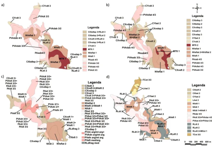
In general, there was a good degree of agreement among all maps. The main soil classes existing in the area were identified by all soil scientists. The soil distribution pattern was similar: Rhodudalfs on plain tops and slopes where the parent material is diabase; Kandiudults and Kandiudalf in the upper third of slopes; and Dystrudepts and Eutrudepts in the lower third of the steeper slopes, where the parent material is siltstone. The four conventional maps are shown in figure 2.

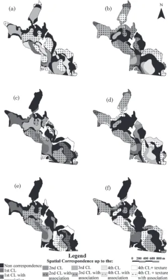
The pairwise superimposition of these maps resulted in the spatial correspondence for each categorical level of BSCS, which is presented as a map (Figure 3). In these maps, the lighter colors indicate areas where the correspondence is in the higher categorical levels.

The comparisons showed a decrease in the spatial correspondence with the increase in categorical level (Figure 4). The main disagreement at the first categorical level (order) occurred among distinctly named MUs, which are morphologically similar and occur associated in the local landscape. As an example, Rhodudalfs and Argiudolls occur on slopes, have a

Figure 2. Conventional soil maps: a) map A; b) map B; c) map C, and d) map D.

clayey texture, high contents of iron oxides, and the same diagnostic B horizon (B nítico). This was similarly observed for a few Rhodudalfs and Eutrudepts, Rhodudalfs and Rhodic Kandiudalfs, Argiudolls and Eutrudepts, Kandiudalfs and Eutrudepts, and Kandiudult and Dystrudepts.

These disagreements were caused by the complexity of soils considered as intergrades between the orders, as well as by the difference in the experience of the soil scientists and the absence of a preliminary legend. In addition, the complexity of the geologic setting of the region contributed to generate several transition areas of soils, which increased the difficulty in defining and delineating each MU. Also, the second categorical level “order” comprises several intermediate sub-levels (e.g.: Nitossolos Argissólicos; Argissolos Nitossólicos etc), resulting in the classification of relatively similar soils in different orders.

At the third categorical level, differences were caused by base saturation. Although there is no subjective component in this measurement, there was great variation in some soil properties within short

Figure 4. Spatial correspondence between conventional soil maps.

(a) (b)

(c) _(d)

(e) _(f)

Figure 3. Spatial correspondence maps between conventional maps: a) A and B; b) A and C; c) A and D; d) B and C; e) B and D; and f) C and D.

distances, e.g., V% and clay activity, as reported by Silva (2000) for this area. According to this author, this interferes with the determination of the soil class, decreasing the efficiency of the mapping process. Therefore, even points close to each other, have significant differences in V%, indicating more than 50 % (eutrophic) in some cases and inferior in others (distrophic). Depending on the point considered by the soil scientist, this would lead to differences in the soil classification.

At the fourth categorical level, the spatial correspondence between maps decreases (Figure 4). One of the main discrepancies was the “abrupt character” variation in some of the Kandiudalf. According to Embrapa (2006), an abrupt textural change is a considerable increase in clay content within a short distance ( 7.5 cm) between the A or E horizon and the underlying B horizon. To identify this characteristic, detailed descriptions and sampling are required, both in soil pits and auger observations, as specified in the BSCS (Embrapa, 2006). However, the study area is used for sugar cane production, which requires deep soil tillage. Therefore, this anthropic effect may have masked the abrupt changes at some points. Another relevant difference at this categorical level was the presence or absence of a latosolic B horizon below the nitic B horizon in the Rhodudalfs. In some cases, the information collected to distinguish the soil classes and their limits was obtained by auger sampling, which causes disturbance in the sampled material, making it hard or impossible to observe the structure, which may have caused this discrepancy. To clear these doubts, it would be necessary to collect material from deeper soil layers, which cannot be reached by conventional augers.

On the other hand, it is obviously inefficient to dig soil pits across the whole area to delineate the limits between the soils (Brady & Weil, 2004). The pedologist therefore needs to compile information on the physical medium (relief, landscape, auger sampling, among others) to make predictions. In this study, the map constructed by each soil scientist was based on his/ his mental concept, on the theoretical knowledge, on an intuitive understanding and on research experiences in the region.

Finally, with regard to the texture, only minor changes in the levels of correspondence of the classification were noted (Figure 4). Is this case, the small divergences observed were related to the clay contents, which are close to the limits between texture classes. Therefore, each scientist decided in which texture class the soil should be allocated.

The smallest agreements, from the second categorical level onwards, were obtained by the comparison of map D with map A (7.0 %) and map D against map B (11.1 %), indicating a greater discrepancy of this map in relation to the others (Figure 4).

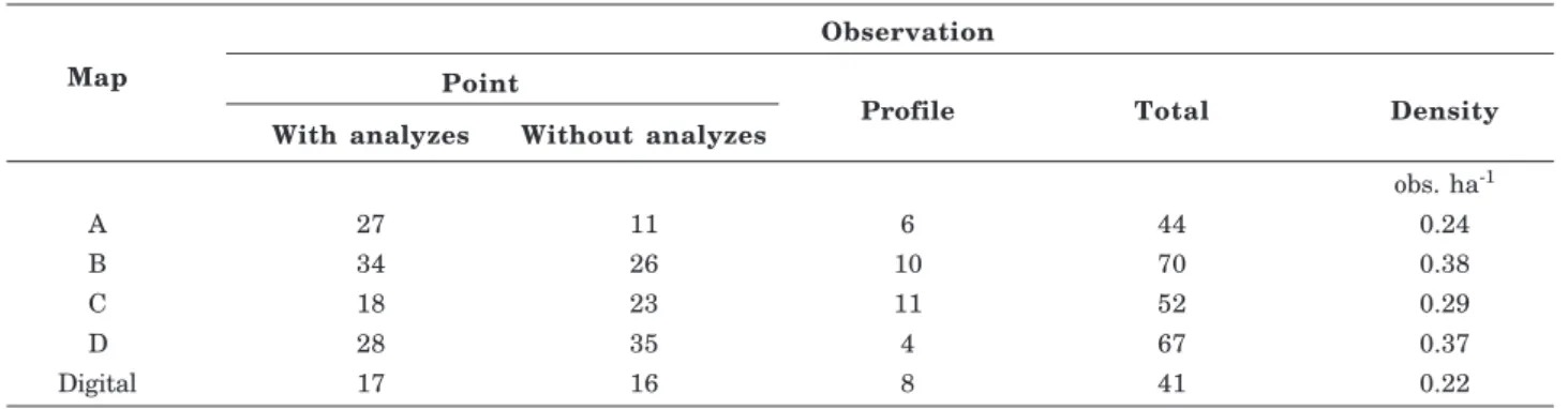
In the construction of the maps B and D, a similar observation density was used (Table 1), which did not result in a high level of correspondence between these maps. This fact may be related to the smaller number of profiles used to draw D than B (Table 1). The construction of all maps satisfied the observation density established by the Normative Procedures for Soil Surveys (Embrapa, 1995), i.e., from 4 to 0.2 observations per hectare (Table 1).

The correspondence of the fourth categorical level plus the texture information among the conventional maps varied from 24.3 (44.4 ha) to 7.0 % (12.7 ha) (Table 2). Silva (2000) compared two soil maps at the same scale, in the same area of Piracicaba, and detected a correspondence of 23 % for the soil classification up to the fourth categorical level. The author reports that one of the reasons for this low level of concordance is the great variability and complexity of soils in the region. Similarly, Bie & Beckett (1973) compared four soil maps of the same area at the same scale, and reported that the maps were considerably distinct.

Despite the disagreement in the soil classification, there was a good correspondence in several properties, although no preliminary soil legend was available for the surveying soil scientists nor correlation studies of

a soil scientist with experience in the area, which are conditions to ensure the quality of any soil survey (Soil Survey Staff, 1993).

Legros (2006) cites the relevance of correlation studies to warrant that surveying teams maintain their methods unchanged over the course of time. According to Rossiter (2000), the correlations should be established by an official institution, aiming to: a) establish a useful and correct mapping legend for the region to be mapped; b) verify whether the MUs are being allocated correctly in the legend.

According to Oliveira (2009), the number of soil scientists in public institutions and the amount of resources destined for soil survey has dropped drastically in the last years in Brazil, which seriously threats the plan to map the soils of the whole territory of the country.

Comparison between conventional soil maps and the digital soil map

The Principal Component Analysis was performed to diminish the redundancy in data for the digital soil mapping. Following the recommendations of Manly (2008), only the components that represented more than 80 % of the total original variance were used. The first principal component represented 41.5 % of the total variance, the second component 19.5 %, the third 14.4 %, the fourth 8.3 %, accounting together for 83.7 % of the total original variance.

Using these four principal components, the area was partitioned using the technique of Fuzzy k-means. To achieve the optimal number of groups, the division

Map

Observation Point

Profile Total Density

With analyzes Without analyzes

obs. ha-1

A 27 11 6 44 0.24

B 34 26 10 70 0.38

C 18 23 11 52 0.29

D 28 35 4 67 0.37

Digital 17 16 8 41 0.22

Table 1. Number of observations per soil map

Categorical level A x B A x C A x D B x C B x D C x D Average

ha (%)

with the smallest performance index was used, which was four groups. Based on the compartment map (Figure 5a) field expeditions were made to collect observations in each group. These observations were based on soil pit examinations, auger prospections, landscape observations and data of soil analyses, to obtain a detailed level of DSM (scale 1: 10,000) of the study area (Figure 5b).

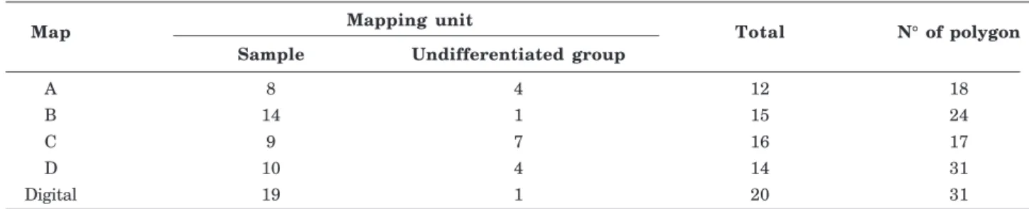
The DSM resulted in a larger number of MUs than the conventional soil maps (Table 3), due to a larger number of compartments in the area. Similarly to the conventional map B, the DSM showed the smallest number of MUs of the undifferentiated group. In the case of the DSM this can be explained by the smaller size of the MUs, increasing the chance of being pure (single-class) units. On the other hand, the C map had larger MUs, and as a consequence they are mostly undifferentiated groups, i.e., MUs with greater heterogeneity.

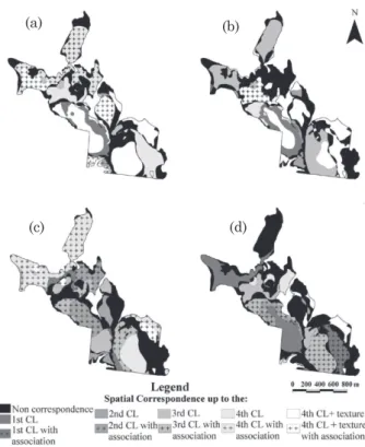
The DSM was compared to each one of the conventional maps and a confusion matrix was made for comparison. These confusion matrices are presented as agreement maps (Figure 6), where light colors indicate agreement at the lower categorical levels.

In the comparisons between the conventional soil maps and the DSM, a decrease in the spatial

correspondence was observed at the more detailed categorical levels, and also from the third to the fourth categorical level (Figure 7).

The disagreements between the DSM and the conventional were similar to those among the conventional maps. At the first level, there were superimpositions of MUs: Rhodudalf and Argiudoll, Eutrudept and Argiudoll, Kandiudalf and Eutrudept, Kandiudult and Dystrudept, and Rhodudalf and Eutrudept. Only this last case differed from the disagreement between conventional soil maps, and occurred close to MUs limits. The area of Rhodudalf was smaller in the DSM than in the conventional maps. In the conventional maps, the area was occupied by Kandiudalf.

According to McKenzie & Austin (1993), geological structures such as dikes and sills can control the pattern of soil distribution. In the study area, the Rhodudalf were formed from a diabase sill (intrusion), therefore being rich in iron oxides, clay rich and red colored at the surface, resulting in lower reflectance (Madeira Neto, 2001). For this reason, soils developed from diabase have a contrasting spectral behavior from Kandiudalf, which are originated from siltstone and fluvial sediments, and as such, contain low amounts of iron oxides and have a medium texture. The 30 x 30 m spatial resolution of the satellite image

Map Mapping unit Total N° of polygon

Sample Undifferentiated group

A 8 4 12 18

B 14 1 15 24

C 9 7 16 17

D 10 4 14 31

Digital 19 1 20 31

Table 3. Characteristics of the mapping units (MUs)

(a) (b)

may have reduced the detailing along the MUs limits, where the disagreement occurred. According to McBratney et al. (2003), the spatial image resolution required to draw a map with a resolution as in this study (1:10,000) would be 10 x10 m.

For the second categorical level of BSCS, the discrepancies were related to the color of Alfissols and

Ultissols (red vs. red-yellow), due to the subjectivity

in the color definition, as reported by Campo & Demattê (2004). At the third categorical level, the differences were related to base saturation and at the

fourth level to the abrupt character of Kandiudalfs and Kandiudults and to the existence of a latosolic B horizon below the nitic B horizon in the Rhodudalf. These disparities were similar to those between the conventional soil maps.

The best levels of final spatial correspondence (4th LC + texture), in relation to DSM, were observed with map A (35.2 %) and map B (28.7 %) (Table 4). Thus, the digital soil map had a greater value of spatial correspondence when compared to the conventional maps A and B, than these two compared to each other. The construction of map A took three days of field work, map B four days, map C three days and map D five days. The digital map took two days. Thus, the DSM required less field observations (Table 1), and still resulted in a greater correspondence with the maps A and B than the maps C and D (Figure 7).

Despite the low coincidence of the DSM for the fourth level + texture when compared to map C (4.3 %) and D (4.0 %), the agreement of map A was also low when compared to map C (6.7 %) and map D (7.0 %) (Figure 7). Nevertheless, in the comparison between DSM and map C, at the fourth categorical level, the correspondence was 31.7 %, which is practically the same as when compared to map B (31.7 %). This means that the variation between conventional soil maps is similar to that between conventional maps and DSM. Therefore, the validations of digital soil maps made by comparing with a single digital map are not correct. In this case, instead of evaluating the digital map error, only the variation intrinsic to any mapping would be observed, independent of being conventional or digital. But also, to compare a digital map with a single conventional map would not be correct and much less satisfactory.

In the comparisons between the DSM and the maps C and D, the lowest values of spatial correspondence were observed at the lower categorical levels. Chagas (2006) compared two digital and one conventional soil map and found a low agreement. For a DSM produced by neural networks, the author found 23.3 % of agreement at the fourth categorical level, and by maximum likelihood the agreement was 12.9 %. The low agreement between the conventional map and the DSMs was assigned to the geological heterogeneity of the area and to problems in the model of environmental correlation used in the DSM. In the same study, the author emphasized that the results would have been different if the conventional soil map had been drawn by another team. This observation was confirmed in this work, where the final spatial correspondence values (fourth level + texture) varied from 35.2 % (map A vs. DSM) to 4.0 % (map D vs. DSM) (Figure 7).

Comparing the average of the spatial correspondence among the conventional maps (Table 2) and between them and the DSM (Table 4), at the different categorical levels of BSCS, similar values

(a) _(b)

(c) (d)

Figure 6. Spatial agreement maps between soil maps: a) Digital and A; b) Digital and B, c) Digital and C; and d) Digital and D.

were observed. Therefore, the average levels of agreement among the conventional maps and between them and the DSM validate the DSM strategy used in this study.

CONCLUSIONS

1. The high complexity of the physical environment increased the difficulty in the process of outlining and classification of the MUs and contributed to the disagreement among the maps and the delineation of MUs in the undifferentiated group.

2. In spite of the disagreements regarding classification, the soil maps (conventional and digital) subdivide the area into polygons and the pedons in one compartment were more similar to each other than to those in the remaining area. This is in line with the main objective of a detailed soil survey.

3. Different scientist teams interact to consolidate a soil map. Since maps are constructed based on the theoretical knowledge and on an intuitive perception and the personal experiences of each soil scientist, it is clearly rather impossible to replicate the representation of the soil delineations. Therefore, it would be practically impossible to represent the work of a pedologist with semi or fully automatized mapping methods by a mathematical model.

4. A similar observation density did not influence the similarity among maps.

5. The DSM has the advantage of eliminating most of the subjectivity of conventional surveys by using quantifiable parameters.

6. This study showed that the DSM coincided better with the maps A and B than with C and D. The average values of spatial correspondence among conventional maps were similar to those between the conventional soils and the DSM.

7. The approach of DSM was adequate to indicate the points of observation (soil profiles, auger observations, etc.). This can save time and other resources.

8. Since the average spatial correspondence among the conventional maps and between these and the DSM

were similar, it is possible to conclude that the DSM produced a map similar to conventional.

9. The disagreements between the maps were mainly related to the inexistence of a preliminary legend and the lack of correlation studies. This reinforced the importance of preparation of these two processes in soil mapping.

ACKNOWLEDGEMENTS

The authors are indebted to Coordenação de Aperfeiçoamento de Pessoal de Nivel Superior (CAPES), for the scholarship of the first author; to FAPESP for funding this research; to the Raízen Group for granting access to the study area; to Dr. Jessica Philippe (Soil Scientist/GIS Specialist, MLRA 12-5 Soil Survey Office, USDA-Natural Resources Conservation Service), for her suggestions and review of the abstract, to people who contributed directly or indirectly to this study and to the soil scientists who supported this project by elaborating the conventional maps of the area.

LITERATURE CITED

BEHRENS, T.; FÖRSTER, H.; SCHOLTEN, T.; STEINRÜCKEN, U.; SPIES, E. & GOLDSCHMITT, M. Digital soil mapping using artificial neural networks. J. Plant Nutr. Soil Sci., 168:21-33, 2005.

BEZDEK, J.; EHRLICH, R. & FULL, W. FCM: The fuzzy c-means clustering algorithm. Comp. Geosci., 10:191-203, 1984.

BOCK, M.; BOHNER, J.; CONRAD, O.; KOTHE, R. & RINGELER, A. SAGA: System for the Automated Geoscientific Analysis. Dept. of Physical Geography, Hamburg, Germany, 2008. URL http://www.saga-gis.org/ en/index.html/. Accessed: May 26, 2011.

BIE, S.W. & BECKETT, P.H.T. Comparison of 4 independent soil surveys by air-photo interpretation, Paphos area (Cyprus). Photogrammetria, 29:189-202, 1973.

BRADY, N.C. & WEIL, R.R. Elements of the nature and properties of soil. 2.ed. New Jersey, Prentice Hall, 2004. 606p.

Categorical level A x Digital B x Digital C x Digital D x Digital Average

ha (%)

CAMPOS, R.C. & DEMATTÊ, J.A.M. Cor do solo: uma abordagem da forma convencional de obtenção em oposição à automatização do método para fins de classificação de solos. R. Bras. Ci. Solo, 28:853-863, 2004. CENTRO NACIONAL DE ENSINO E PESQUISA AGRONÔMICA - CNEPA. Levantamento de reconhecimento de solos do Estado de São Paulo. Rio de Janeiro, Ministério da Agricultura, 1960. 637 p. (Boletim, 12)

CHAGAS, C.S. Mapeamento digital de solos por correlação ambiental e redes neurais em uma bacia hidrográfica no domínio de mar de morros. Viçosa, MG, Universidade Federal de Viçosa, 2006. 223 p. (Tese de Doutorado) CHAGAS, C.S.; JÚNIOR, W.C. & BHERING, S.B. Integração

de dados do Quickbird e atributos de terreno no mapeamento digital de solos por redes neurais artificiais. R. Bras. Ci. Solo, 35:693-704, 2011.

DALMOLIN, R.S.D. Faltam pedólogos no Brasil. B. Inf. SBCS, 24:13-15, 1999.

DEMATTÊ, J.L.I. A pedologia direcionada ao manejo de solos. B. Inf. SBCS, 24:16-17, 1999.

DEMATTÊ, J.A.M.; GENÚ, A.M.; FIORIO, P.R.F.; ORTIZ, J.L.; MAZZA; J.A. & LEONARDO, H.C.L. Comparação entre mapas de solos obtidos por sensoriamento remoto espectral e pelo método convencional. Pesq. Agropec. Bras., 39:1219-1229, 2004.

DELARMELINDA, E.A.; WADT, P.G.S.; ANJOS, L.H.C.; MASUTTI, C.S.M.; SILVA, E.F.; SILVA, M.B.; COELHO, R.M.; SHIMIZU, S.H. & COUTO, W.H. Avaliação da aptidão agrícola de solos do Acre por diferentes especialistas. R. Bras. Ci. Solo, 35:1841-1853, 2011. DIMITRIADOU, E.; HORNIK, K.; LEISCH, F.; MEYER, D. &

WEINGESSEL, A. e1071: Misc Functions of the Department of Statistics (e1071), TU Wien, r package version 1.5-18, 2008. Available at: <http://cran.r-project.org/web/packages/e1071/index.html> Accessed: May 15, 2011.

EMPRESA BRASILEIRA DE PESQUISA AGROPECUÁRIA -EMBRAPA. Centro Nacional de Pesquisa de Solos. Manual de métodos de análise de solo. 2.ed. Rio de Janeiro, Embrapa Solos, 1997. 212p.

EMPRESA BRASILEIRA DE PESQUISA AGROPECUÁRIA -EMBRAPA. Centro Nacional de Pesquisa de Solos. Sistema brasileiro de classificação de solos. 2.ed. Rio de Janeiro, Embrapa Solos, 2006. 306p.

EMPRESA BRASILEIRA DE PESQUISA AGROPECUÁRIA -EMBRAPA. Centro Nacional de Pesquisa de Solos. Procedimentos normativos de levantamentos pedológicos. Brasília, Embrapa - SPI, 1995. 101p.

ESRI. ArcGIS Desktop Developer Guide ArcGIS 9. Redlands, ESRI Press, 2006. CD ROM.

FELDWISCH, N. Hangneigung und Bodenerosion.cBoden und Landschaft - Schrif tenreihezurc Bodenkundec Landes kultur und Landschaft sokologie der Justus-Liebig-Universitat Gieben, Inst. fürLandeskultur, 1995. 152p.

FOCHT, D. Influência do avaliador no resultado da classificação de terras em capacidade de uso. Piracicaba, Escola Superior de Agricultura “Luiz de Queiroz”, 1998. 79p. (Dissertação de Mestrado)

HARTEMINK, A.E. & McBRATNEY, A.B. A soil science renaissence. Geoderma, 148:123-129, 2008.

HORN, B.K.P. Hillshading and the reflectance map. Proc. IEEE, 69:14-47, 1981.

HUDSON, B.D. The soil survey as paradigm-based science. Soil Sci. Soc. Am. J., 56:836-841, 1992.

LEPSCH, I.F. Manual para levantamento utilitário do meio físico e classificação de terras no sistema de capacidade de uso. Campinas, Sociedade Brasileira de Ciência do Solo, 1991. 175p.

JACOMINE, P.K.T. É preciso investir na formação de novos pedólogos. B. Inf. SBCS, 24:21-22, 1999.

JENNY, H. Factors of soil formation: a system of quantitative pedology. New York, McGraw-Hill, 1941. 281p.

JOAQUIM, A.C.; BELLINASO, I.F.; DONZELLI, J.L.; QUADROS, A.D. & BARATA, M.Q.S. Potencial e manejo de solos cultivados com cana-de-açúcar. In: SEMINÁRIO COPERSUCAR DE TECNOLOGIA AGRONÔMICA, 6., Piracicaba, 1994. Anais... Piracicaba, Centro de Tecnologia Copersucar, 1994. p.1-10.

KER, J. C. O futuro da pedologia no Brasil. B. Inf. SBCS, 24:18-21, 1999.

LAGACHERIE, P. & McBRATNEY, A.B. Spatial soil information systems and spatial soil inference systems: Perspectives for digital soil mapping. In: LAGACHERIE, P.; MCBRATNEY A.B. & VOLTZ, M., eds. Digital soil mapping: An introductory perspective. New York, Elsevier, 2007. p.3-22.

LEGROS, J-P. Mapping of the soil. Enfield, Science Pubishers, 2006. 411p.

MADEIRA NETTO, J.S. Comportamento espectral dos solos. In: MENESES, P.R. & MADEIRA NETTO, J.S., eds. Sensoriamento remoto: Reflectância dos alvos naturais. Brasília, Universidade de Brasília, 2001. p.127-154. MANZATTO, C.V. & ASSAD, E.D. Zoneamento

agroecológico da cana-de-açúcar para a produção de etanol e açúcar no Brasil: Seleção de terras potenciais para a expansão do cultivo. B. Inf. SBCS, 35:21-23, 2010. McBRATNEY, A.B.; MENDONÇA-SANTOS, M.L. & MINASNY, B. On digital soil mapping. Geoderma, 117:3-52, 2003.

McKENZIE, N.J. & AUSTIN, M.P. A quantitative australian approach to medium and small scale surveys based on soil stratigraphy and envirormental correlation. Geoderma, 57:329-355, 1993.

MENDONÇA-SANTOS, M.L. & SANTOS, H.G. The state of the art of Brazilian soil mapping and prospects for digital soil mapping. In: LAGACHERIE, P.; McBRATNEY, A.B. & VOLTZ, M., eds. Digital soil mapping: An introductory perspective. Amsterdam, Elsevier, 2007. p.39-55. MANLY, B.J.F. Métodos estatísticos multivariados: Uma

introdução. 3.ed. Porto Alegre, Bookman, 2008. 229p. MEZZALIRA, S. Folha Geológica de Piracicaba: SF 23-M 300.

São Paulo, Instituto Geográfico e Geológico do Estado de São Paulo. 1966. 1 mapa. Escala 1:100.000

MOORE, I.D.; GESSLER, P.E.; NIELSEN, G.A. & PETERSON, G. Soil attribute prediction using terrain analysis. Soil Sci. Soc. Am. J., 57:443-452, 1993.

NANNI, M.R. Dados radiométricos obtidos em laboratório e no nível orbital na caracterização e mapeamento de solos. Piracicaba, Escola Superior de Agricultura “Luiz de Queiroz”, 2000. 365p. (Tese de Doutorado)

NANNI, M.R. & DEMATTÊ, J.A.M. Spectral reflectance methodology in comparison to traditional soil analysis. Soil Sci. Soc. Am. J., 70:393-407, 2006.

NOLASCO-CARVALHO, C.C.; FRANCA-ROCHA, W. & UCHA, J.M. Mapa digital de solos: Uma proposta metodológica usando inferência fuzzy. R. Bras. Eng. Agr. Amb., 13:46-55, 2009.

OLIVEIRA, J.B. As séries e o novo sistema brasileiro de classificação de solos. Tem-se condições de gerenciar o seu estabelecimento? Available: <http://200.20.158.8/ blogs/sibcs/?p=188#more-188>. Accessed: Nov. 16, 2009. OLIVEIRA, J.B. & PRADO, H. Carta pedológica semidetalhada de Piaracicaba. Campinas, IAC, 1989. Escala: 1:100.000.

OLIVEIRA, V.A. O Brasil carece de novos pedólogos. B. Inf. SBCS, 25:25-28, 1999.

R DEVELOPMENT CORE TEAM. R: A Language and Environment for Statistical Computing, R Foundation for Statistical Computing, Vienna, 2008. Available: <http:/ /www.R-project.org, ISBN 3- 900051-07-0>. Accessed: Dec.16, 2010.

REUSSER, D. Tiger: Analysing time series of grouped errors, r package version 0.1, 2009. Available: <http://cran.r-project.org/web/packages/tiger/index.html>. Accessed: May 20, 2011.

ROSSITER, D.G. Methodology for soil resource inventories. 2.ed. Amsterdam, International Institute for Aerospace Survey & Earth Sciences (ITC), 2000. 132p.

SANTOS, R.D. Quem defende a extinção do pedólogo não conhece a sua importância. B. Inf. SBCS, 24:23-24, 1999. SECRETARIA DE ECONOMIA E PLANEJAMENTO - SEP. Governo do Estado de São Paulo -. Plano cartográfico do Estado de São Paulo. Folhas 78/89 Toledo e 79/89 Costa Rica. São Paulo, 1977. Mapa, escala 1:10.000.

SHI, X.; LONG, R.; DeKETT, R. & PHILIPPE, J. Integrating different types of knowledge for digital soil mapping. Soil Sci. Soc.Am. J., 73:1682-1692, 2009.

SILVA, E.F. Mapas solos produzidos em escalas e épocas distintas. Piracicaba, Escola Superior de Agricultura “Luiz de Queiroz”, 2000. 177 p. (Tese de Doutorado)

SOIL SURVEY STAFF. Soil survey manual. Washington, USDA-SCS. U.S. Gov. Print. Office, 1993. 437p. (Agric. Handbook, 18)

SOIL SURVEY STAFF, NATURAL RESOURCES CONSERVATION SERVICE, UNITED STATES DEPARTMENT OF AGRICULTURE. Soil Survey Geographic (SSURGO) Database for Essex County, Vermont. Available: <http://soildatamart.nrcs.usda.gov>. Accessed: Feb. 17, 2012.

STORY, M. & CONGALTON, R.G. Accuracy assessment: A user‘s perspective. Photogram. Eng. Remote Sens., 52:397-399, 1986.

TANRÉE, D.; HOLBEN, B.N. & KAUFMAN, Y.J. Atmospheric correction algorithm for NOAA-AVHRR products: theory and application. IEEE Trans. Geosci. Remote Sens., 30:231-248, 1992.

WOLD, H. Systems under indirect observation. Amsterdam, Elsevier, 1982. 668p.

WOOD, J.D. The geomorphological characterization of digital elevation models. Leicester, University of Leicester, 1996. 187p. (Tese de Doutorado)

XIE, X. & BENI, G. A validity measure for fuzzy clustering. IEEE T. Pattern Anal. Applic., 13:841-847, 1991. ZEVENBERG, L.W. & THOME, C.R. Quantitative analysis of

landsurface topography. Earth Surf. Proc. Landf., 12:47-56, 1987.