Volume 1 Number 2 (2012): Pages 195-211
ISDS Article ID: IJDS12080803
Modelling seasonal farm labour demand:
What can we learn from rural Kakamega
district, western Kenya?
Vincent
Canwat
*Department of Agriculture and Rural Development, International Institute of Social Studies, The Hague, the Netherlands
Abstract
Seasonality of agricultural activities causes fluctuation in the quantity of labour consumed by these activities, and yet many rural labour studies in developing countries still treat labour demand in agriculture as if it is the same across different farm operations. To unearth the amount of information hidden by this aggregated analysis, labour demand for specific farm operations was estimated based on data collected from Kakamega District. This analysis shows that increasing household size increases labour demand for planting, weeding and harvesting. Increasing the share of elderly household members has a negligible effect on labour demand for farm activities except for land preparation, with which it is positively related. Participation of primary school-going children in farm activities is the highest in planting and harvesting. Participation in off-farm employment seems to increase labour demand only during peak seasons. The area planted appears to have an insignificant effect on labour demand for land preparation. Planting sugar cane appears to reduce labour demand for weeding and primary processing, but planting tea increases labour demand for planting. Mechanising land preparation only reduces labour demand for land preparation, but it seems to be offset by other labour-intensive farm operations. The distance from water source is positively related to labour demand for land preparation, but the distance to the market is negatively related to labour demand for weeding and harvesting. These observations point to the need for supporting and investing in technological and organisational innovations in agriculture.
Keywords:Modelling, Seasonal labour demand, Rural Kakamega district
Copyright © 2012 by the Author(s) – Published by ISDS LLC, Japan
International Society for Development and Sustainability (ISDS)
Cite this paper as: Canwat, V. , Modelling seasonal farm labour demands: What can we learn
from rural Kakamega district, western Kenya? , International Journal of Development and
1.
Introduction
Labour plays important economic and social roles in any economy. It is one of the key factors of production as well as a source of livelihood to billions of people worldwide, especially the absolute landless farmers who are neither renting land nor sharecropping, but are endowed with physical labour power and skills accumulated over time through experience and traditions; the landless with smaller stock of livelihood assets supplemented by occasional engagement in non-farm activities and; the near-landless owning and renting smaller pieces of land in addition to wage labour work they do during peak cropping seasons (FAO, 1986). The stock and quality of labour that households have in terms of their size, educational attainment, and know-how as well as health status constitute human capital, which can be allocated to different sectors of the labour market to meet livelihood and production needs of households as well as labour requirements for the production of goods and services by firms and states (Takane, 2008:1; Schneider, 2005:3).
The different sectors of the labour market in developing countries to which labour is allocated comprise formal and informal sectors of the urban labour market as well as agricultural and non-agricultural sectors of the rural labour market (Mazumdar, 1989:7).
The agricultural sector of the rural labour market, as Mazumdar : noted, comprises large−scale and small−scale subsectors. Mazumdaralso observed that the large−scale subsector consists of plantations and large family farms, which depend heavily on hired labor, much as factories do; however, the small−scale subsector relies not only on hired workers, but also on the self−employed. The self−employed consists of owner−operators and tenants, who often supplement their farm incomes by trading in environmental goods such as forest and other wild products and small-scale production of items such as furniture, baskets, mats, craft goods, and others (Arnold, 1994:1-20; Mazumdar,1989:8). These activities are labour intensive, and they greatly depend on entrepreneurs and members of their families for labour, but incomes they earn from these activities are particularly crucial during seasonal decline in the supply of food and cash-crop income and in periods of drought as well as other emergencies (Arnold, 1994:1-20). Whereas plantations and large farms usually employ labour on long-term contracts ranging from a season to many years, small farms hire on a casual , day−to−day basis Mazumdar, : . Mazumdar also argued that the enforcement of minimum wage laws is sometimes possible in the large−scale agricultural sector because some of their hired workers are organised, but such institutional influence is rare among wage workers in small−scale agriculture, where the labor market is mainly governed by the law of supply and demand and heavily influenced by social custom.
Unlike in the non-agricultural sector, labour allocation in the agricultural sector is greatly affected by seasonality of agricultural activities. This seasonality influences the quantity of labour consumed by agricultural activities and consequently, the wage rates of farm labour, but the more advanced an economy is, the less extensive is the seasonality because of more advancement and investment in technologies and organisational innovations, known for reducing seasonality like irrigation machinery and new institutional arrangements between farm and non-farm sectors that allow labour mobility (Engerman and Goldin, 1991:3). In spite of the clear effects of agricultural seasonality on labour, particularly in less advanced countries, many scholars continue to ignore seasonality in economic analysis of labour demand. Many writers consider labour demand for hired labour as being the same across different farming activities (Odoemenem and Odom, 2010: 323). And works ofBabikir and Babiker (2007), Bowlus and Sicular (2003), and others are victims of this simplistic analysis. In their study, Odoemenem and Odom analysed farm labour demand for different farm operations, but their analysis was restricted to hired labour demand. They neglected key farm operations like land preparation and processing. Instead, they considered additional operations such as thinning and fertilizer application, which are less significant among small-scale farmers. This paper contributes towards bridging this information gap, and it analyses labour demand for land preparation, planting, weeding, harvesting, processing and marketing in the rural Kakamega District. The paper is
2.
Analytical framework
Approaches for modelling rural labour demand draw a lot from the conventional neoclassical theory, but deviate from it in regards to the assumptions held about the market. According to the neoclassical perspective, prices are exogenous, farmers participate in the market, and the decisions pertaining to production and consumption are separately or recursively made. This implies that labour availability to farm production activities is not affected by time spent on leisure (Benjamin, 1992:290). Leisure comes after work. Therefore, the production problem of the product ( ) with price ( ); two variable factors x and l (labour) with prices and w respectively and; fixed and farm characteristics ( ) is profit maximisation expressed as max�= − − subject to production technology, � , , ; =0, and the reduced form of the production problem defines labour demand function ( ) as, , , , (Sadoulet and de Janvry, 1995: 145). Under the same conditions, Sadoulet and de Janvry expressed the consumer problem with an agricultural good� and price ; manufactured good � and price ; disposable income and consumer household characteristics � as a utility maximisation problem with a utility function max� , � �(� ,� ; �) subject to budget constraint, � + � = , and derived demand function for goods as �� =�� , , ; � , where �= ,
At the same time, they considered a worker problem with home time �, time worked �, total time endowment available and worker characteristics as a utility maximisation problem with a utility function max�, �(�, ; ) subject to income constraint, = �, and time constraint, � + � = or full income � + = , and derived home time demand function as � =� , ; . They derived a combined consumption/work problem as a utility function max� , � , � �(� ,� ,�; ℎ) subject to full time constraint, + � + � =�∗+ , and time constraint � + �= , and generated a demand function of goods as �� =�� , , , ∗; ℎ , where � = , , ; y∗= − − + and ℎ are characteristics of the household.
However, when the market is imperfect, production and consumption decisions are no longer recursively (separately) made. Under this circumstance, production and consumption decisions are simultaneously made based on endogenous prices ( ∗) as follows: = ( ∗, ); �∗= �∗ �; �=�( ∗, ∗, ℎ) and ∗, ∗ depend on exogenous prices , household characteristics , ℎ, exogenous transfer T, and credit K in case credit is a constraining factor, and substitution for ∗and ∗ generate reduced forms = , , ℎ,�, for production, and �=� , , ℎ,�, for consumption (Sadoulet and de Janvry, 1995: 145) .
Based on this theoretical framework and the works of Benjamin (1992) and Bowlus and Sicular (2002), the model for assessing factors affecting farm labour demand was specified as: =�0+�1 ��+ �2 ��+�3�� +�4 � +�5 +�6 �+�7��+�8 +�, where, �0,�1 ,�2,�3,�4,�5,�6,�7,�8 are model parameters and � is the error term. L is labour demand defined as the total person days spent working on cultivated land by both the household members and hired labour; �� is the household size defined as number of persons in a household, and a household is considered as a group of people eating from a common pot or
a fraction of household members with no formal education, with primary education, secondary education and those with tertiary education, including vocational, college and university education. A is the area planted or cultivated measured in acres. K is capital expenses measured as expenses in hiring animal traction or tractor services. � is the crop enterprise. Main enterprises considered are tea and sugarcane growing enterprises measured as dummies. �� is the participation in off-farm employment measured by asking whether household members are engaged in off-farm employment or not, is the distance from the nearest market measured in metres, and� is the error term.
3.
Materials and methods
3.1.
Area of study
This paper is based on a study conducted in Kakamega District, the provincial headquarter of western Kenya. The district has a bimodal rainfall pattern, which gives rise to two distinct seasons of long rains from March to June with a peak in May and short rains from July to September with a peak in August (Kilavuka, 2003:19). The drier period runs from December to February (Ibid). The district covers 1275 km2 of arable land, 577 km2 of cultivated area and 322 km2 of gazetted forested land, which preserves water catchment areas and supplies wood fuels. The district has a population density of 522 people per square kilometre, with a birth rate of 44 per 1000 population, death rate of 14.3 per 1000 population and the total fertility rate of 5.1 percent (Ibid). Up to 62 percent of the population is engaged in agriculture, 8 percent in rural self-employment, 20 percent in wage self-employment, 2 percent in urban self-employment and 8 percent in other sectors (Kakamega District Development Plan, 2002). Major crops grown are maize, beans, tea and sugarcane. Other crops include bananas and horticultural crops. Main livestock kept are cattle, sheep, goats and poultry. The district was chosen because it was the location of BIOTA project under which this study was conducted. A sample population of 121 farm households was selected based on stratified random sampling. Four strata of Ikolomani, Shinyalu, Ileyo, and Lurambi divisions were generated based on local government administrative units. A simple random sampling was conducted within each of the strata to obtain the target sample size. These farm households comprised thirty BIOTA contact farmers and other ninety one households in the vicinity of the contact farmers.
3.2.
Data collection
0 .1 .2 .3 .4
De
n
sity
y
0 2 4 6
Ln labour used in processing
0 .2 .4 .6
De
n
sity
0 1 2 3 4
Ln labour used in harvesting
0
.1 .2 .3 .4
.5
1 2 3 4 5 6
Ln Labour used in weeding
De
n
sity
y
0 .1 .2 .3 .4 .5
0 1 2 3 4
Ln labour used in planting
0 .2 .4 .6
De
n
sity
y
0 1 2 3 4
Ln labour used in Land preparation
0
.2
.4 .6
De
n
sity
y
3 4 5 6 7
Ln Total labour used in the season
De
n
sity
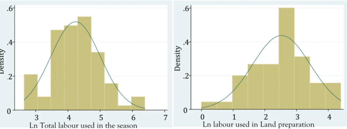
Figure 1. Histogram and density plot for total labour used in the season
Figure 3. Histogram and density plot for labour used in planting
Figure 4. Histogram and density plot for labour used in weeding
Figure 5. Histogram and density plot for labour used in harvesting
Figure 6. Histogram and density plot for labour used in processing
The data was summarised as descriptive statistics and presented in Tables 1a and 1b below.
Table 1a. Descriptive Statistics of Endogenous (Dependent) Variables.
Variable Mean STD Min Max
Total labour used in the season ( in person-days)
Ln (Total labour used in the season)
Labour used in land preparation
Ln(Labour used in land preparation)
Labour used in planting
Ln (Labour used in planting)
Labour used in weeding
Ln (Labour used in weeding)
Labour used in harvesting
Ln (Labour used in harvesting)
Labour used in primary processing
95.12 4.24 18.24 2.52 8.42 1.80 34.22 3.05 9.75 1.86 24.48 97.71 0.77 17.20 0.91 8.44 0.79 44.33 0.98 11.84 0.88 36.02 14.00 2.64 1.00 0.00 1.00 0.00 2.00 0.69 1.00 0.00 1.00 594.00 6.39 81.00 4.39 49.00 4.89 296.00 5.69 76.00 4.33 220.00
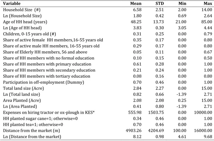
Table 1b. Descriptive Statistics of exogenous (independent) variables
Variable Mean STD Min Max
Household Size (#) Ln (Household Size)
6.58 1.80 2.51 0.42 2.00 0.69 14.00 2.64 Age of HH head (years)
Ln (Age of HH head) Children, 0-15 years old (#)
Share of active female HH members,16-55 years old Share of active male HH members, 16-55 years old Share of Elderly HH members, 56 and above Share of HH members with no formal education Share of HH members with primary education Share of HH members with secondary education Share of HH members with tertiary education Participation in off-employment (Dummy)
48.25 3.83 0.31 0.35 0.29 0.05 0.10 0.61 0.21 0.08 0.70 13.73 0.30 0.25 0.17 0.17 0.11 0.15 0.28 0.24 0.16 0.46 21.00 3.05 0.00 0.00 0.00 0.00 0.00 0.00 0.00 0.00 0.00 85.00 4.44 0.79 0.80 0.80 0.67 0.50 1.00 1.00 0.80 1.00 Total land size (Acre)
Ln (Total land size) Area Planted (Acre)
2.84 0.82 2.08 2.27 0.66 2.08 0.00 -1.39 0.25 15.00 2.71 15.00
Ln (Area Planted) 0.41 0.80 -1.39 2.71
Expenses on hiring tractor or ox-plough in KES* 555.98 1503.75 0.00 10000.00
HH planted sugar cane=1; otherwise=0 0.34 0.46 0.00 1.00
HH planted tea=1; otherwise=0 Distance from the market (m) Ln (Distance from the market)
0.70 4903.26 8.12 0.46 4204.69 0.98 0.00 100.00 4.61 1.00 16000.00 9.68
4.
Results and discussion
This section presents and discusses the results of the model estimation and test. The models were estimated and tested for misspecification, endogeneity and heteroskedasticity problems as well as seperability assumption. The levels of multicollinearity were also measured. These statistical operations were conducted in STATA.
4.1.
Model estimation and test
Model misspecification is a source of bias, which causes a serious model problem, if not detected and mitigated. This bias arises from the omission of key independent variables or their functions, and it leads to bias and inconsistent ordinary least square estimators (Wooldridge, 2009: 300). For this reason, the estimated labour demand models were subjected to a specification test. Firstly, demand models oflabour used in land preparation, planting, weeding, harvesting, primary processing, and the total amount of labour consumed during the season were estimated as functions of household size, share of elderly household members, shares of household members with primary and tertiary education, off-farm employment, acreage planted, expenses on animal traction and tractor services and cash crops grown. Secondly, these models were subjected to Ramsey Reset Test of Model Specification. However, the test failed to reject null hypotheses that the estimated labour demand models had no omitted variables, except in land preparation labour demand model (Table 4). Land preparation labour demand was then specified as a function of household size, access to credit, the share of elderly household members, the share of household members with tertiary education, expenses on hiring animal traction and tractor services, and the distance from the main road, water source as well as interaction between the age of household head and soil type in the study area.
The levels of multicollinearity were also measured. Multicollinearity is one of the assumptions of classical linear regression. It arises when regressors have perfect linear relationships between them. Multicollinearity increases standard error leading to inaccurate hypothesis testing. This analysis used Variance Inflation Factor (VIF) command to test for the degree of multicollinearity. The test found that the level of multicollinearity was far below the critical level. All model variables scored tolerance level higher than 0.6 and model VIF of 1.35 and below (table 2). Therefore, the models seem to be free of the multicollinearity problem.
Endogeneity is another source of bias tested for. Based on past research work, household size and area cultivated were known to be possible sources of endogeneity bias. These variables can pose serious risk of
endogeneity when their measurements are not done well, but endogeneity is also a problem when other key variables are omitted from the model (Bowlus and Secular, 2003: 565; Wooldridge, 2009: 300). These variables were, therefore, tested for exogeneity using Hausman test, and the test confirmed their exogeneity
Table 2. Multicollinearity Test for Cropping Activity Labour Demand Model
Variables VIF 1/VIF Variables LPD Model VIF 1/VIF
HH members- tertiary educ. 1.66 0.603 HH members- tertiary educ. 1.39 0.718
Ln (Area Planted) 1.56 0.639 Share of the elderly 1.29 0.775
Planted sugar cane 1.51 0.662 Cost of hiring ox. & tractor 1.27 0.788
Cost of hiring ox. & tractor 1.43 0.702 Ln (Age household head*Alfisol) 1.18 0.849
HH members-primary educ. 1.38 0.723 Ln (Distance to main road) 1.09 0.914
Ln(Distance to market) 1.29 0.773 Receive credit 1.03 0.969
Planted tea 1.25 0.797 Ln (Distance to water source) 1.02 0.977
Share of the elderly 1.09 0.913 Ln (Household size) 1.02 0.981
Ln (Household size) 1.09 0.913
Participate in off-employment
1.07 0.932
Mean VIF=1.35
Mean VIF=1.16
Table 3. Hausman Test for Exogeneity
Variable Model (1) Model (2) Model (3) Model (4)
Endogenous Variable Ln HH size Ln Total labour Ln Area planted Ln Total labour
Exogenous Variable
Ln (Household size) - 0.315 - -
Ln (Area planted) - - - 0.0539
Ln (Age of household head 0.0273*** - - -
Ln (Total land size) - - 0.765*** -
Residual1 0.191
Residual 2 - - - 0.220
Cost of hiring ox. & tractor -0.0000101 0.000286*** 0.000138*** 0.000231***
HH members- tertiary educ. -0.413 -1.324** -0.467 -1.474***
HH members-primary educ. -0.112 -0.298 -0.339 -0.289*
Share of the elderly -1.839*** 1.452** 0.884* 1.538**
Planted sugar cane 0.171** -0.191 0.433*** -0.297*
Planted tea 0.036 0.418** 0.177 0.405*
Participate in off-employment
0.0718 0.303** 0.086 -0.302
Ln (Distance to market 0.047 -0.145* 0.141** -0.148*
Constant (Intercept) 0.193 4.373*** -1.463*** 5.275***
R-Squared 0.471 0.387 0.656 0.368
Adjusted R-Squared 0.412 0.312 0.618 0.290
Prob. > F 0.000 0.000 0.000 0.000
To test for the violation of equal variance assumption, Breusch-Pagan/Cook-Weisberg test for heteroskedasticity was used. All the estimated labour demand models passed the test, except for processing and weeding labour demand models (Table 4). They were then estimated using regression with heteroskedasticity-consistent standard errors approach.
The validity of the seperability assumption was also tested. Seperability assumption—which means the simultaneous making of consumption (labour supply) and production (labour demand) decisions by farm households—holds under perfect labour market conditions. However, it is widely known that labour markets in developing countries, like Kenya and others, are very far from being perfect, and the seperability assumption appears not to hold. Thus, the model was tested for this assumption. The test followed the methodology used by Benjamin (1992). This methodology is grounded on the premise that when labour market is imperfect, household composition becomes an important factor determining farm labour use. Therefore, by estimating labour demand model (5) and testing whether the effects of household size and household composition were jointly equal to zero, seperability assumption was not accepted, except for primary crop processing labour (Table 4). This appears to confirm labour market imperfection, and it implies that the conventional method of analysing labour demand may not be appropriate for this analysis.
4.2.
Model explanation
This section explains how household size, household composition, household education, participation in off-farm employment, land cultivated, crop planted, capital expenses and location characteristics affect overall labour demand and labour demand of different operations in the cropping cycle.
Household size is significantly and positively related to labour demand for planting, weeding and harvesting, but insignificantly related to labour demand for primary processing and land preparation. An increase in household size by one percent increases labour demand for planting, weeding and harvesting by 0.439 percent, 0.531 percent, and 0.675 percent respectively. The magnitude of the coefficient increases from planting to harvesting, showing increasing labour demand from planting to harvesting time. The fact that labour demand is positively related to household size confirms earlier findings and the theoretical suggestion that when production and consumption decisions are simultaneously made, increase in household size drives down the cost of labour (shadow price) because of increased labour supply by farm households (Bowlus and Sicular, 2002:573). Household size has an insignificant effect on labour demand for primary processing and land preparation, probably because they are off-peak activities that require less household participation. Some household members may engage in off-farm activities, but they concentrate on farm activities during peak periods, like harvesting or weeding time (Paris et al., 2009:174).
feeding is concerned. They are idle, but need care and feeding. As Bowlus and Sicular, : noted, …an extra child requires care and so may divert time from other uses, it also increases the number of mouths to feed and so may induce the parents to work more hours in the field . (owever, they also suggested that such analytical results would be different if it was conducted separately for the healthy elderly household members, who actively participate in farm activities, and the unhealthy ones, who need care and divert labour from farm production (Bowlus and Sicular, 2002:574). Even though they may participate in other activities that require less strength, the labour demand model suggests that their labour contribution is negligible.
Primary and tertiary education are negatively related to labour demand of cropping activities, but the effects of primary education are only significant for labour demand for planting and harvesting. This is probably because majority of household members are primary school-going children, who normally perform light tasks, like ferrying produce and others relevant to their capacity. This observation seems to confirm previous studies. For example, Ajoke and colleagues (2011:130) found that the majority of children supporting their family members with agricultural activities in Nigeria participate mainly in planting (96%) and harvesting (92%) as compared to other activities like processing (80%), weeding (76%), transplanting % , and thinning % . They maintain that the level of children s participation in a particular agricultural activity is indirectly proportional to the demand of that activity as far as strength, skill and safety are concerned.
Increasing the share of household members with tertiary education by one unit reduces labour demand for land preparation, planting, weeding, harvesting, and processing by 1.048%, 1.361%, and 1.349%, 1.721%, 1.129%, and 1.829% respectively. The effects of tertiary education on weeding and primary processing labour demand are significant at 1% significant level, while for others they are significant at 5% and 10%. Households with the higher share of tertiary education graduates seem to be more effective in reducing labour demand for weeding and harvesting, probably because they are aware of and use chemical weed control techniques and primary processing equipment. This suggestion is consistent with the view that education enhances agricultural productivity because of its complementarily with new technologies (Lockerhead and Lau, 1980: 38). Education is related to access to information about new technologies (Illukpitiya and Gopalakrishnan, 2004:324), and there is a positive linkage between farmer s education and adoption of new technology (Strauss, 1990: 323).
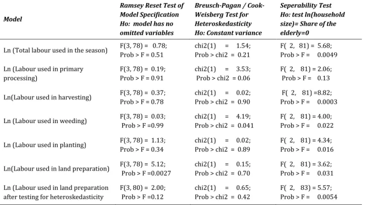
Table 4: Test for model misspecification, heteroskedasticity and seperability assumption
Model
Ramsey Reset Test of Model Specification Ho: model has no omitted variables
Breusch-Pagan / Cook- Weisberg Test for Heteroskedasticity Ho: Constant variance
Seperability Test Ho: test ln(household size)= Share of the elderly=0
Ln (Total labour used in the season) F(3, 78) = 0.78; Prob > F = 0.51
chi2(1) = 1.54; Prob > chi2 = 0.21
F( 2, 81) = 5.68; Prob > F = 0.0049
Ln (Labour used in primary processing)
F(3, 78) = 0.19; Prob > F = 0.91
chi2(1) = 3.53; Prob > chi2 = 0.06
F( 2, 81) = 2.06; Prob > F = 0.13
Ln(Labour used in harvesting) F(3, 78) = 0.37; Prob > F = 0.78
chi2(1) = 0.02; Prob > chi2 = 0.90
F( 2, 81) =8.82; Prob > F = 0.0003
Ln (Labour used in weeding) F(3, 78) = 0.03; Prob > F =0.99
chi2(1) = 4.19; Prob > chi2 = 0.041
F( 2, 81) = 4.00; Prob > F = 0.022
Ln (Labour used in planting) F(3, 78) = 1.13; Prob > F = 0.34
chi2(1) = 0.02; Prob > chi2 = 0.89
F( 2, 81) = 4.34; Prob > F = 0.016
Ln(Labour used in land preparation) F(3, 78) = 5.12; Prob > F =0.0027
chi2(1) = 0.15; Prob > chi2 = 0.70
F( 2, 81) = 3.62; Prob > F = 0.031
Ln (Labour used in land preparation after testing for heteroskedasticity
F(3, 80) = 2.00; Prob > F =0.12
chi2(1) = 0.65; Prob > chi2 = 0.42
F( 2, 83) = 5.57; Prob > F = 0.0054
Area cultivated is positively related to labour demand, but it has an insignificant effect on labour demand for land preparation. Increasing the area planted by one percent increases labour demand for planting by 0.225%, for weeding by 0.203%, harvesting by 0.194% and processing by 0.287%. This finding is expected and has theoretical consistency. The area planted has an insignificant effect on labour demand for land preparation, probably because land preparation is an off peak farm operation. Related to land preparation is the interaction between soil type and the age of the household head. This interaction reduces labour demand for land preparation. This is probably because of the ease of cultivating alfisol, which encourages participation of even the elderly. Meanwhile, ultisol is difficult to work for the elderly, and so this discourages their participation.
a ti on a l Jour n a l of D ev el opm en t a n d Sus ta in a b il ity Vol .1 N o.2 ( 20 12 ): 1 95 w ww .isds n e t.c om Ta b le 5 . L a b ou r d e ma n d m o de l e stima tio n r e sul ts p ende n t iab le In d ep ende n t (E x o genou s) V a r iab les Intercept
Ln (household size) Share of the elderly
HH members-primary education
HH members- tertiary education
Participate in off-farm employment Ln (Area Planted) Planted sugar cane
Planted tea Cost of hiring ox. &
tractor Ln (Distance to
market) ota l la bou r d in t h e a son 0.399** 1.426** -0.264 -1.361** 0.284* 0.159 -0.287* 0.367* 0.000251*** -0.151* 4.597*** L a bou r d in nting 0.439** 0.915 -0.732** -1.349** 0.232 0.225** -0.121 0.684*** -0.0000542 -0.0251 1.427* L a bou r d in e d in g 0.531** 1.284 -0.235 -1.721*** 0.363* 0.203* -0.435** 0.372 0.000346*** -0.214*** 3.628*** L a bou r d in rve st in g 0.675*** 1.156 -0.552* -1.129* 0.206 0.194* -0.156 0.297 0.000289*** -0.0305 0.905 L a bou r d
in ary ss
in g 0.405 1.419 0.133 -1.829*** 0.442* 0.287* -0.701* 0.287 0.000339*** -0.322*** 3.995*** iab le
Ln (household size) Share of the elderly Received credit HH members- tertiary education Ln (Distance to main road)
Ln (Area Planted) Ln (Distance to water source Ln (Age of household head)*Alfisol Cost of hiring Ox-plough & tractor Cont bou r u se d a
nd para
Expenses on hiring animal traction and tractor services is positively and significantly related to labour demand for weeding, harvesting and processing, but is negatively and significantly related to labour demand for land preparation. It is also positively related to planting, but with insignificant effects. Increasing capital expenses by 1000 Kenya shillings reduces labour demand for land preparation by 0.227%, but it increases overall labour demand by 0.251%, labour demand for weeding by 0.346%, harvesting by 0.289%, and for primary processing by 0.339%. Reduction of labour demand as a result of using animal traction and tractor conforms to production theory, which points to the substitution effect of capital use on labour. The use of tractor and animal traction as mechanization technologies displaces labour and reduces labour-to-land ratio (Viegas, 2003:37, 42). Meanwhile, a positive relationship between capital expenses and labour demand in other farm activities suggests that the use of animal traction and tractors is restricted only to land preparation and to some extent planting. This observation seems to be supported by the work of Panin (1994:206). Panin noted that increased tractorisation was equally accompanied by increased labour use because tractor use was limited to land preparation and planting, where labour saving was realised, but offset by manually operated labour intensive activities of weeding, harvesting, and threshing.
The distance from the market is negatively related to labour demand, but the relationship is insignificant as far as labour demand for planting and harvesting is concerned. However, the distance from the water source is positively and significantly related to labour demand for land preparation. Increasing the distance to the market by 1% reduces labour demand for weeding by 0.214% and for harvesting by 0.322%. However, increasing the distance from water source by one percent increases labour demand for land preparation by 0.134%. The negative effect of the distance from the market on labour demand for land preparation suggests that the closer households are to the market, the more likely that they are to engage in off-farm activities, leading to labour diversion from farm activities. Babikir and Babiker (2007: 341) and Anim (2011: 28) found similar effect in their studies of labour demand in Sudan and South Africa respectively. They attribute this effect to a greater possibility in working off-farm, which diverts labour from farm activities. The positive linkage between the distance from water source and labour demand is attributed to the fact that the further the water source, the more time is diverted from farm activities.
5.
Conclusion
This paper estimated labour demand functions for cropping stages. These functions show how labour demand for land preparation, planting, weeding, harvesting, and primary processing activities are affected by household size, household composition, household education, participation in off-farm employment, area
planted, crop planted, capital expenses and location characteristics.
Increasing household size was found to increase labour demand during peak periods of planting, weeding
and harvesting only. Increasing the share of household members of 56 years and above seems to have negligible effect on labour demand for all the cropping stages except for land preparation, with which it is positively related, mainly because the elderly household members withdraw labour for their care and direct
seems to be the highest in planting and harvesting, which demand less from them in terms of strength and skills. Participation in off-farm employment seems to increase labour demand only during peak seasons. Area planted appears to have an insignificant effect on land preparation labour demand, probably because it is an off-peak farm operation. Labour demand for land preparation appears to be influenced by factors associated with human strength. Planting sugar cane appears to reduce labour demand for weeding and primary processing, but planting tea increases labour demand for planting. Mechanising land preparation only is not enough, because labour saved from its mechanization seems to be offset by other labour-intensive farm operations. The distance from water source is positively related to labour demand for land preparation, but the distance to the market is negatively related to labour demand for weeding and harvesting.
These observations have implications for both technological and organisational innovations. The government and other development agencies might need to promote and support appropriate technologies that deepen farm mechanization from land preparation to primary processing using appropriate technology or other labour-reducing technologies. Less time-dependent activities may need to be planned for off-peak seasons and new institutional arrangements may need to be established between farm households and off-farm enterprises so that surplus labour available during slack periods can be absorbed in off-off-farm activities.
Acknowledgements
I am very grateful for the professional advice provided by Professor Michael Grimm during the preparation of this article and Elena Kouzovova for proof reading the manuscript.
I am very thankful to Professor Holm Müller and Professor Mathias Becker for their professional guidance and advice during the data collection and preparation exercises. I am also thankful for materials and other supports rendered by Frank Mussgnug, Thuweba Diwani, Elisabeth Nambiro, and John Achieng during the research process.
Of course, a heartfelt gratitude goes to KAAD and BIOTA Project for their financial support. Lastly, I say thank you to everyone, who in one way or another contributed to this article.
References
Agénor, P. (2005), The Analytics of Segmented Labor Markets , Discussion Paper Series. Manchester
University, Manchester: Centre for Growth and Business Cycle Research, Economic Studies, available online
at: http://www.socialsciences.manchester.ac.uk/disciplines/economics/research/discussionpapers/pdf/
EDP-0529.pdf (accessed 15 October 2012).
Agénor, P.R. and P. J. Montiel (1996), Development Macroeconomics, Princeton University Press, Princeton,
USA.
Anim, F.D.K , Factors Affecting Rural (ousehold Farm Labour Supply in Farming Communities of
Arnold, E.M. , Nonfarm employment in small-scale forest-based enterprises: Policy and environmental
issues , working paper, Environmental and Natural Resources Policy and Training Project EPAT . University
of Oxford, UK, pp. 1-20.
Babikir, O.M. and Babiker, B.). , The Determinants of Labour Supply and Demand in )rrigated Agriculture: A Case Study of the Gezira Scheme in Sudan , African Development Review, Vol. 19 No. 2, pp. 335– 349.
Benjamin, D. (ousehold Composition, Labor Markets, and Labor Demand: Testing for Separation in
Agricultural (ousehold Models , Econometrica, Vol. 60 No. 2, pp. 287-322.
Bowlus, J.A. and T. Sicular (2002), Moving toward markets? Labor allocation in rural China , Journal of
Development Economics, Vol.71, pp. 561– 583.
De Vries, S.C., Van de Ven, G.W.J., Van )ttersum, M.K. and Giller, K.E. , The Production-ecological
Sustainability of Cassava, Sugarcane and Sweet Sorghum Cultivation for Bioethanol in Mozambique , GCB Bioenergy, Vol. 4, pp. 20–35.
Engerman, S. and Goldin, C. , Seasonality in Nineteenth Century Labour Markets , NBER Historical working paper 20, available at: http://www.nber.org/papers/h0020 (accessed 18 June, 2012).
FAO (Food and Agriculture Organisation) (1986), The dynamics of Rural Poverty, FAO, Rome, Italy.
Gwyer, G.D. , Trends in Kenyan Agriculture in Relation to Employment ,The Journal of Modern African
Studies, Vol. 11 No. 3, pp. 393-403.
Illukpitiya, P. and Gopalakrishnan C. , Decision-making in Soil Conservation: Application of a
Behavioral Model to Potato Farmers in Sri Lanka , Land Use Policy, Vol. 21 No. 4, pp. 321–331.
Kakamega District Development Plan (2002), Kakamega District Development Plan 2002-2008, Ministry of
Planning and National Development, Kenya.
Kilavuka, J.M. (2003), A comparative Study of the Socio-economic Implications of Rural Women, Men, and
Mixed Self-help Groups: A case of Kakamega District . )n Ossrea ed. Gender Issues Research Report Series No ,
available online at: http://publications.ossrea.net/images/stories/ossrea/girr-20.pdf, (accessed 5 May 2012).
Lockheed, E.M., Jamison, T. and Lau L.J. (1980 , Farmer Education and Farm Efficiency: A Survey , Economic
Development and Cultural Change, Vol. 29 No. 1, pp. 37-76.
Odoemenem, I.U. and Odom, L.N. (2011), Some Factors Affecting the Demand for (ired Labor: A Case Study
of Maize Farmers of Benue State, Nigeria , Current research Journal of Social Sciences, Vol. 2 No. 6, pp. 322-326.
Ajoke, O., Olaide, S.J. and Oluwakemi, L.B. , Children s Participation in Agricultural Activities in the
Adopted Villages of the )nstitute of Agricultural Research and Training, Nigeria , Journal of Rural Social Sciences, Vol. 26 No. 2, pp. 126–136.
Panin, A. , Empirical Evidence of Mechanization Effects on Smallholder Crop Production Systems in
Botswana , Agricultural Systems, Vol. 41, pp. 199-210.
Sadoulet, E. and De Janvry (1995), Quantitative Development Policy Analysis, The Johns Hopkins University
Schneider, S. (ed.) (2005), (uman capital is the key to growth: Success Stories and Policies for , Current Issues: Global growth Centres. Frankfurt am Main: Deutsche Bank Research, available online at: http://www.dbresearch.com/PROD/DBR_INTERNET_ENPROD/PROD0000000000190080.PDF (accessed 16 October 2012).
Strauss, J., Barbosa, M., Teixeira, S., Thomas, D. and Junior, R.G. , Role of Education and Extension in
the Adoption of Technology: A Study of Upland Rice and Soybean Farmers in Central-West Brazil ,
Agricultural Economics, Vol. 5, pp. 341-359.
Takane, T. , Labor Use in Smallholder Agriculture in Malawi: Six Village Case Studies, African Study
Monographs, Vol. 29 No. 4, pp. 183-200.
Paris, T.R., Chi, T.T.N., Rola-Rubzen, M.F. and Luis, J.S. , Effects of Out-migration on Rice-Farming
Households and Women Left Behind inVietnam , Journal of Gender, Technology and Development, Vol. 13 No. 2,
pp. 169–198.
Viegas, E. , Agricultural mechanization: managing technology change , in Da Costa, (., Piggin, C., Da
Cruz, C.J. and Fox, J.J. (Ed.), Agriculture: New Directions for a New Nation — East Timor (Timor-Leste), ACIAR
Proceedings No. 113.