A TUTORIAL ON HYPERCUBE QUEUEING MODELS AND SOME PRACTICAL APPLICATIONS IN EMERGENCY SERVICE SYSTEMS
Fernando Chiyoshi
1, Ana Paula Iannoni
2and Reinaldo Morabito
3*Received February 19, 2010 / Accepted December 27, 2010
ABSTRACT.This paper presents some extensions and applications of hypercube queueing models to describe server-to-customer type Emergency Service Systems. The classical hypercube is a well-known spatially distributed queueing model effective in analyzing these systems, based on Markovian analysis ap-proximations. Experience has shown that each real life Emergency Service System may have its own unique characteristics so that each system may require a particular hypercube queueing model incorporating those characteristics. Some of these distinctive characteristics are considered in the extensions presented in this tutorial such as dispatch policy based on random selection of the server to take an incoming call; partial cooperation among servers whereby depending on where the call is coming from, some servers cannot take the call; servers with additional workload coming from walk-in nonemergency customers such as in customer-to-server systems; existence of calls requiring the dispatch of more than one server; existence of more than one type of servers in the system, for instance paramedical and medical units in emergency medi-cal systems. In this study, we present a set of these models based on the smallest non-trivial service systems. For each model, the construction of the system of equations for equilibrium hypercube state probabilities and the evaluation of particular operational characteristics are described.
Keywords: hypercube queueing model, emergency service systems, toy-models, server-to-customer systems.
1 INTRODUCTION
Emergency Service Systems (ESS) provide emergency assistance to incidents, protecting and ensuring public health and safety, and they can be classified as either customer-to-server systems or server-to-customer systems. In the first case, service units are considered immobile in the sense that customers must travel to where servers are located, whereas in the latter the servers
*Corresponding author
1Department of Production Engineering, COPPE/Universidade Federal do Rio de Janeiro, RJ, Brazil. E-mail: [email protected]
2Ecole Centrale Paris, Laboratoire Genie Industriel, France. E-mail: [email protected]
are mobile, that is, they travel to the scene of the emergency. In this case, the system is also called an emergency response system; some examples are requests for urgent medical assistance, police patrol as well as fire combat units and emergency repairs. In these systems, mobile servers are more accurately modeled as distinguishable from one another in the sense that the servers are spatially distributed in the region and have different characteristics (e.g., different preferential regions and mean service times), they share the system workload due to cooperation, and their workloads may be different and may vary according to the location of the servers.
Surveys on probabilistic location models that use mobile servers in ESS can be found, for exam-ple, in Larson & Odoni (1981), Kolesar & Swersey (1986), ReVelle (1989), Swersey (1994), Owen & Daskin (1998), Brotcorneet al. (2003), Marianov & Serra (2003), Goldberg (2004), ReVelle & Eiselt (2005) and Galvao & Morabito (2008). The hypercube queueing model develo-ped by Larson (1974) and extended by other authors (Swersey, 1994) is an effective descriptive model for designing and planning server-to-customer ESS. The basic idea of the model is to ex-pand the state space description of a queueing system with multiple servers in order to represent each server individually and incorporate more complex dispatch policies. The model takes into account geographical and temporal complexities of the region under consideration and it is ap-propriate to analyze coordinated (centralized) systems, where the user requiring service calls the central station of the system and the system manager dispatches a server to service the call. If there is no server available, the call either enters a waiting line until a server becomes available, or it is transferred to another ESS.
The name hypercube derives from the state space describing the status of the servers. Each server can be free (0) or busy (1) in a given time instant. A particular state of the system is given by the entire listing of servers that are free and busy. For example, the state{110}corresponds to a 3-server system, with server 1 free and servers 2 and 3 busy (note that {110}describes the state of the servers from right to left). Taking this into account, the state space is given by the vertices of a cube. If the system has more than three servers, we have a hypercube (Larson, 1974). Given the system configuration, the hypercube model is able to evaluate a variety of performance measures relevant for decision-making, either region-wide or for each server or region. These include server workloads, mean user response times, fraction of dispatches of each server to each region, among others. In solving location problems in which the best locations of the servers are searched, the hypercube model is used as a descriptive tool to evaluate the quality of a given set of locations.
other major emergencies (Larson, 2004). Other references related to applications and extensions of the hypercube model can be found in Halpern (1977), Jarvis (1985), Battaet al.(1989), Swer-sey (1994), Chiyoshiet al. (2000, 2003), Galv˜aoet al. (2003, 2005), Saydam & Aytug (2003), Costa (2004), Iannoni & Morabito (2007), Luque (2007) and Atkinsonet al.(2006, 2008).
Each system involved in the practical applications of the hypercube queueing model has its own distinctive characteristics. The objective of this paper is to present a set of models to show how these characteristics are handled and how the associated output measures are evaluated. To that end, we use the smallest, non-trivial structures that incorporate the characteristics of systems under analysis. These structures, referred to as “toy-models”, are used to provide useful insights into problems of interest, but are mostly unable to directly address the complexity of real world ESS.
We start discussing single dispatch hypercube models in which it is assumed that the arriving calls at the ESS require the dispatching of only one server (Section 2). In Section 2.1, we review the basic single dispatch model considering both infinite and finite (possibly zero) capacity waiting lines with either homogeneous or non-homogeneous servers. Then the centralized model with random dispatches is described (Section 2.2), where all servers share the same home location and there are no preferences as to the server to be dispatched to service a call, which is inspired in the case of an urban SAMU (Service d’Aide M´edicale Urgente) studied in Takedaet al.(2007). In Section 2.3, we present the partial backup model in which it is assumed that each region of the ESS is the home location of a server, and that a server can only service calls from its preferential region and from the second closest region. The model considers a zero capacity waiting line system with homogeneous or non-homogeneous servers. This is the case of some emergency medical systems on motorways, as for example in the SAU’s (Sistema de Atendimento ao Usu´ario– highway’s user response system) studied in Mendonc¸a & Morabito (2001), Iannoni & Morabito (2007) and Iannoniet al.(2009, 2011).
Then in Section 3 we analyze multiple dispatch hypercube models which consider that some arriving calls at the ESS require the simultaneous dispatching of two or more servers. Some examples appear in emergency medical systems, police patrol systems and fire emergency sys-tems. For instance, in emergency medical systems, the multiple dispatching of ambulances is needed especially when incidents involving several victims require two or more ambulances for assistance and transport. In policy patrol systems, frequently two police patrols with one or two police officers are sent to the same event to work together, for example, one offering cover to the other in case of danger. In fire control systems, more than one unit is usually dispatched to control the fire according to the proportion of the incident and the number of required pieces of equipment and personnel (Swersey, 1994).
callers). This case appears, for example, in police deployment systems where a police patrol could be busy in an event as a result of something illegal that the police officer sees from the patrol car (i.e., an event that was not received by the call operations center, namely PIA – patrol initiated activity), as studied in Larson & Mcknew (1982). Another example appears in highway emergency medical systems where a third status of the ambulances refers to eventual assistance to patients requesting service at the ambulance bases, as studied in Iannoni & Morabito (2007) and Atkinsonet al.(2008).
In Section 3.3, we consider the multi-dispatch model with differentiated servers. In several ESS, a dispatch policy that considers different types of servers according to the type of vehicle, per-sonnel or equipment required by the call type are common. For example, in emergency medical systems in urban areas, the ambulances can be either advanced support vehicles (ASV) or basic support vehicles (BSV), and the calls are divided into two classes: advanced calls (preferenti-ally serviced by an ASV) and basic calls (preferenti(preferenti-ally serviced by a BSV) (Brandeau & Larson, 1986; Takedaet al., 2007). Another example appears in emergency medical systems on highways with medical vehicles and ambulances. The medical vehicles transport specialized medical per-sonnel (e.g., doctors, nurses and rescuers), some basic medications and tools for pre-clinical care. Conversely, the ambulances transport the patients, medical personnel, clinical and pre-hospital care equipment and other heavier equipment (e.g., hardware breakers, fire control equipment, etc.), as studied in Iannoni & Morabito (2007). Finally, in Section 4 we present some concluding remarks and discuss some opportunities for future research.
2 THE SINGLE DISPATCH HYPERCUBE MODEL
2.1 The basic model
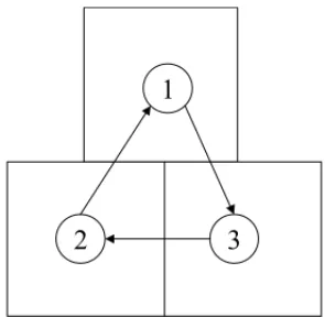
For the purpose of building the toy-models, we take a simple network consisting of only three atoms (i.e., pre-defined sub regions of the ESS region) connected by a one-way ring road. It is assumed that the centroids of the atoms are located at the vertices of an equilateral triangle with sides of unit length, as shown in Figure 1. The inter-atoms travel distance matrix for this network is shown in Table 1.
1
3
2
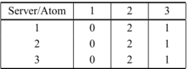
Table 1– Inter-atom travel distances. From To Atom
Atom 1 2 3
1 0 2 1
2 1 0 2
3 2 1 0
We start by considering the basic hypercube queueing model as known in the literature (Larson, 1974; Larson & Odoni, 1981). For this model, we assume that each atom is the home location of a server, and a fixed-preference dispatch policy, with preferences set according to shortest distances is in use. The preference matrix is shown in Table 2.
Table 2– Server dispatch preferences. Atom Server Preferences
1st 2nd 3rd
1 1 2 3
2 2 3 1
3 3 1 2
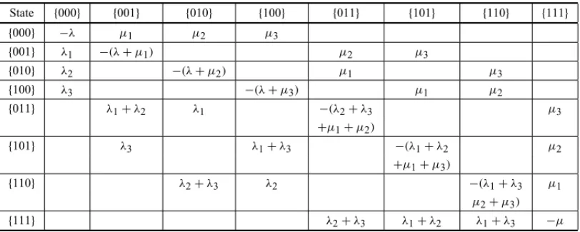
The hypercube state probabilities are defined by a set of flow-balancing equations built around the hypercube states. To that end, we represent these states through a triad of 0/1 variables (0 – free, 1 – busy) of the form{i j k}, each one associated with a server, with the correspondence of variable to the server made from right to left. In addition, we define:
• λj as the arrival rate of calls from atom j; • µi as the service rate of server (or unit)i; • λ=λ1+λ2+λ3as the total arrival rate;
• µ=µ1+µ2+µ3as the total service rate.
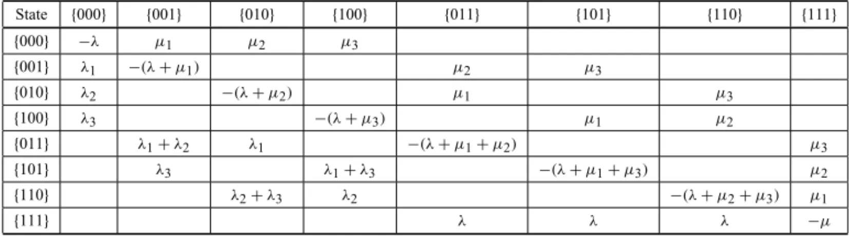
In order to build the balance equation for a given state, say{011}, we argue as follows: the system leaves state{011}if a call arrives, or a service is completed by server 1 or 2. The rate associated with this transition is(λ+µ1+µ2)P{011}. Conversely, the system enters state{011}: (i) from state{001}when a call arrives from atoms 1 or 2 (in accordance with Table 2); (ii) from state
{010}when a call arrives from atom 1; or (iii) from state{111}when a service is completed by server 3. The rate associated with this transition is(λ1+λ2)P{001} +λ1P{010} +µ3P{111}. By arguing that in steady state the transition rates of the system out of and into a given state must be equal, we write the balance equation for state{011}as:
(λ+µ1+µ2)P{011} =(λ1+λ2)P{001} +λ1P{010} +µ3P{111}
or
The transition rate equilibrium equations around other states of the system can be built in a similar fashion (Chiyoshiet al., 2000, 2003). The full coefficient matrix of the system of equations for the zero capacity waiting line hypercube model (i.e., a loss system with no waiting room) is shown in Table 3. Figure 2 illustrates the possible states for this example on the vertices of a cube, states {000},{001}, . . . ,{111}. As aforementioned, if this example had more than three servers, the corresponding figure would be represented by a hypercube.
Table 3– Coefficients matrix of the system of equations for the basic model with zero waiting line.
{ } { } { } { } { } { } { } { }
{ } −λ µ µ µ
{ } λ −(λ+µ ) µ µ
{ } λ −(λ+µ ) µ µ
{ } λ −(λ+µ ) µ µ
{ } λ +λ λ −(λ+µ +µ ) µ
{ } λ λ +λ −(λ+µ +µ ) µ
{ } λ +λ λ −(λ+µ +µ ) µ
{ } λ λ λ −µ
000
111
001
011 010
101 100
110
Figure 2– Cube representing the possible states of the system.
It is worth noticing that the entries in the coefficient matrix of Table 3, except for the diagonal entries, represent the transition rates from column states to row states. The diagonal entries are the symmetrics of the transition rates of the system out of the corresponding states. Each row of this matrix displays the coefficients of the flow rate balance equation built around the state shown in the leftmost column.
standard procedure is to replace one of the equations by an equation of probabilities normaliza-tion condinormaliza-tion. For the zero capacity waiting line hypercube, this equanormaliza-tion is simply:
P{000} + P{001} + ∙ ∙ ∙ +P{111} =1.
The state probabilities for the zero capacity waiting line can be adjusted to handle non-loss systems with an arbitrary number of waiting spots. Suppose room is added to accommodate one additional call. Then the system must be augmented with an additional state, say{S4}, with four calls in the system, three being serviced and one waiting in queue. Since the state{111}is already in balance with the adjacent states of the hypercube, the transitions between states{111}
and{S4}must also be in balance, so that:
λP{111} =µP{S4} or P{S4} =ρP{111},
whereρ=λµis the average workload of the system.
When a new state is added to the hypercube states, the set of numbers P{000}, . . . ,P{111}, P{S4} is no longer a proper probability distribution since the sum of these numbers can be greater than 1. This condition can be restored via sum-one normalization. Similar procedure can be used to handle a waiting line with any capacity, augmenting the system with additio-nal states{S4},{S5},{S6}, . . .For an infinity capacity waiting line, the equation of probabilities normalization condition becomes (Chiyoshiet al., 2000):
P{000} +P{001} + ∙ ∙ ∙ +P{111}
(1−ρ)=1.
To show the ways in which the output measures of a hypercube models are derived from its state probabilities, we consider two such measures, namely server workload and dispatch frequencies. The workload of a serveriis defined as the ratio between its output (production) and its capacity. It can be evaluated as the fraction of time the server is busy by summing the probabilities of the states in which serveri is busy. The workload of server 1 for the non-zero capacity waiting line would be:
ρ1=P{001} +P{011} +P{101} +P{111} +P{Q},
whereQis an additional state in which there is at least one call waiting for service.
Another major output measure is the server dispatch frequencies. The dispatch frequency of unit ito atomj(denoted by fi j) is defined as the fraction of a call associated with the dispatch of unit i to atom j. These frequencies can also be derived from the state probabilities. For a non-zero capacity waiting line, they have two components, the first associated to unqueued calls (denoted by fi j[u]) and the second associated to queued calls (denoted by fi j[q]). If we consider the dispatch of unit 1 to atom 2 to service unqueued calls, for instance, its frequency can be evaluated as the joint probability that: (i) server 1 is free and server 2 (preferential server of atom 2) is busy, and (ii) the incoming call is originated from atom 2:
The dispatch frequency of server 1 to atom 2 to service a queued call is given by the joint proba-bility that: (i) all servers are busy, given by P{111} +P{Q}, (ii) server 1 is the first of all busy servers to become free, given byµ1/µ(see the Appendix), and (iii) atom 2 is the origin of the first waiting call for service. Therefore we have:
f12[q]=(P{111} +P{Q}) (λ2/λ)(µ1/µ)
for the dispatch frequency of unit 1 to atom 2 to service a queued call.
The toy-models can be coded into smallad hoccodes which can serve (at least) two purposes. The first one is to layout the basic logic larger codes to deal with more complex problems. The other is to “play” with the models in a “what if” sort of approach in order to assess the way in which the systems definition parameters affect its output measures.
We start by looking at the basic characteristics of a double homogeneous system (homogeneous in both demand and service rates) by fixingλ1=λ2=λ3=0.5 andµ1=µ2=µ3=1.0. The state probabilities for this system are shown in Table 4. The row labeledLossof this table shows the state probabilities associated with the zero capacity waiting line. The state probabilities adjusted for the infinite capacity waiting line are shown in the following row (labeled Q(∞)).
Table 4– Hypercube states probabilities.
State {000} {001} {010} {100} {011} {101} {110} {111} {Q} Loss 0.239 0.119 0.119 0.119 0.090 0.090 0.090 0.134 –
Q(∞) 0.211 0.105 0.105 0.105 0.079 0.079 0.079 0.118 0.118
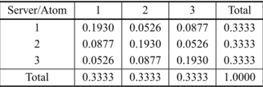
The dispatch frequencies for the infinite waiting line are shown in Table 5. The symmetric nature of the model is reflected in these frequencies: (i) all servers have the same total dispatch frequency, (ii) all atoms have the same total frequency of units dispatched to them, and (iii) the dispatch vectors have the same pattern for all units, in which dispatch frequencies decrease according to whether the unit is dispatched as preferential, first or second backup unit.
Table 5– Dispatch frequencies for infinite waiting line.
Server/Atom 1 2 3 Total
1 0.1930 0.0526 0.0877 0.3333 2 0.0877 0.1930 0.0526 0.3333 3 0.0526 0.0877 0.1930 0.3333 Total 0.3333 0.3333 0.3333 1.0000
first unit is twice the rate of units 2 and 3, keeping the same total rate (µ1 =1.50,µ2 =0.75, µ3 =0.75). The relevant data for the infinite waiting line are shown in Tables 6 and 7. It can be observed that the faster unit has lower workload and it is dispatched more frequently than the slower units. Although the slower units have the same service rate, unit 2 is seen to have a lower occupation rate than unit 3. This difference is due to the fact that unit 2 is the first backup of the faster and less busy server (unit 1).
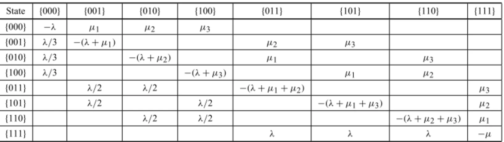
2.2 The centralized model with random dispatches
In this toy-model, it is assumed that all service units share the same home location and there are no preferences as to the unit being dispatched to service a call. In building the system of equations for equilibrium state probabilities, we must argue differently from the previous model. The transition rate, from say, state{000}to state{001}, must be 1/3 of the total arrival rate since the random dispatch will select server 1, on average, 1/3 of the time out of three free units. In a similar way, the transition rate from state{001}to state{011}must be 1/2 of the total arrival rate because, in this case, we have two free servers to choose randomly from, and, in the long run, server 2 will be chosen half the time out of two free units.
In order to build the balance equation for a given state, say{011}, we argue the following: the system leaves state{011}if a call arrives, or a service is completed by server 1 or 2. The rate associated with this transition is (λ+µ1+µ2)P{011}. Conversely, the system enters state {011}: (i) from state{001}half the time a call arrives in the system; (ii) from state{010}half the time a call arrives or (iii) from state{111}when a service is completed by server 3. The rate associated with these transitions are(λ/2)P{001} +(λ/2)P{010} +µ3P{111}. The steady state flow balance reasoning leads to the following equation for state{011}:
(λ+µ1+µ2)P{011} =(λ/2)P{001} +(λ/2)P{010} +µ3P{111}
or
(λ/2)P{001} +(λ/2)P{010} −(λ+µ1+µ2)P{011} +µ3P{111} =0.
Table 8– Coefficient matrix of the system of equations for the centralized model with random dispatches.
{ } { } { } { } { } { } { } { }
{ } −λ µ µ µ
{ } λ/ −(λ+µ ) µ µ
{ } λ/ −(λ+µ ) µ µ
{ } λ/ −(λ+µ ) µ µ
{ } λ/ λ/ −(λ+µ +µ ) µ
{ } λ/ λ/ −(λ+µ +µ ) µ
{ } λ/ λ/ −(λ+µ +µ ) µ
{ } λ λ λ −µ
In evaluating the dispatch frequencies of unqueued calls (fi j[u]), the random nature of the dispatch policy must be taken into account, and appropriate formulas constructed. For example, the dis-patch frequency of server 1 to atom 2 is obtained by combining the probability that the incoming call comes from atom 2, which isλ2/λwith: (i) 1/3 of the probability that all servers are free; (ii) half the probability that server 1 is one of two free servers; and (iii) the probability that server 1 is the only free server. The resulting expression is thus:
f12[u]=(λ2/λ)
(1/3)P{000} +(1/2) P{010} +P{100}+P{110}
The dispatch frequencies for servicing queued calls are not affected by server preferences, de-pending only on arrival pattern and the probability that a given server is the first one to complete service when all servers are busy. They can be evaluated following the same procedure described for the basic model.
A centralized system can be viewed as a stage in the natural growth of a small emergency medical service built based on a local hospital. The growing demand of such a system both in volume of the calls and covered area can be faced by increasing the number of ambulances located in the hospital. The time may come in which it is asked as to the effect of decentralizing the system to improve its performance in terms of, say, response time. For an example of a related situation in practice, the reader is referred to the case of theSAMU-Campinas studied in Takedaet al. (2007). This problem can be addressed by looking at the average travelled distances in both centralized and decentralized models. The average travelled distance per call can be evaluated as the weighted sum of the (home location of the) units to atom distances, the weighting factors being the dispatch frequencies.
average of the distances in Table 1 weighed by the dispatch frequencies of Table 5, the average travelled distance per call for the decentralized model turns out to be 0.58.
Table 9– Unit to atom distances matrix for the centralized model.
Server/Atom 1 2 3
1 0 2 1
2 0 2 1
3 0 2 1
2.3 The partial backup model
The next toy-model we look at is a partial backup model. It assumes that each atom is the home location of a server, and that a server can only service calls from its preferential atom and from the second closest atom. Server 1, for example, can take calls from atoms 1 and 2, but not from atom 3. The corresponding dispatch matrix is shown in Table 10.
Table 10– Server dispatch prefe-rences for the partial backup model.
Atomi Server preferences
1st 2nd
1 1 2
2 2 3
3 3 1
It may be assumed that the decision to not dispatch server 1 to atom 2 is based on the existence of a secondary ESS to handle such a call and a zero capacity waiting line model seems appropriate. Some practical examples appear in SAUs on highways, as the ones ofAnjos do Asfaltostudied in Mendonc¸a & Morabito (2001) andCentroviasstudied in Iannoni & Morabito (2007). The flow equations of the system can be built in a way similar to that used for the basic model. Care must be taken, however, in determining some of the upward transition rates. Consider state{011}, for instance, where both servers 1 and 2 are busy and server 3 is free. A call from atom 1 will not change the state of the system because it cannot be serviced by server 3, the only server available (Table 10); the call will be lost. The upward transition rate from state{011}to state{111}will therefore be:(λ2+λ3). The flow equation around state{011}will be:
(λ2+λ3+µ1+µ2)P{011} =(λ1+λ2)P{001} +λ1P{010} +µ3P{111}.
The full coefficient matrix for this model is shown in Table 11.
will be evaluated as the joint probability that the incoming call has originated in atom 2, server 2 is busy and server 1 is free:
f12[u]=(λ2/λ)(P{010} +P{110})
The dispatch frequency of serveri to atom j is defined simply as the fraction of all dispatches that send serveri to atom j; so we would expectP
i,j f [u]
i j =1. Due to lost calls, however, the dispatch frequencies based on the formula above will add up to less than one; in fact, they will add up to the fraction of calls that are serviced by the system, leaving out the lost calls. For this reason, a second step is required in which results from the first step are normalized to sum one.
Table 11– Coefficient matrix of the system of equations for the partial backup model. State {000} {001} {010} {100} {011} {101} {110} {111}
{000} −λ µ1 µ2 µ3
{001} λ1 −(λ+µ1) µ2 µ3
{010} λ2 −(λ+µ2) µ1 µ3
{100} λ3 −(λ+µ3) µ1 µ2
{011} λ1+λ2 λ1 −(λ2+λ3 µ3
+µ1+µ2)
{101} λ3 λ1+λ3 −(λ1+λ2 µ2
+µ1+µ3)
{110} λ2+λ3 λ2 −(λ1+λ3 µ1
µ2+µ3)
{111} λ2+λ3 λ1+λ2 λ1+λ3 −µ
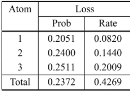
The most distinctive characteristic of this model is the fraction of lost calls, both per atom and system wide. To show how the fraction of lost calls can be evaluated, we work out an instance in whichλ1 =0.4,λ2 =0.6,λ3=0.8 andµ1=µ2 =µ3=1.0. By solving the corresponding system of linear equations, we obtain the hypercube state probabilities as shown in Table 12. From these equilibrium probabilities, the dispatch frequencies are evaluated (Table 13).
Table 12– Hypercube state probabilities for the partial backup model. State {000} {001} {010} {100} {011} {101} {110} {111} Prob 0.1979 0.1018 0.1120 0.1425 0.0799 0.1259 0.1148 0.1252
Table 13– Dispatch frequencies.
Server/Atom 1 2 3 Total
The first thing to observe in Table 13 is the total dispatch frequency of 0.7628, which corres-ponds to the fraction of calls that are serviced by the system, resulting in a fraction of lost calls of 0.2372. The dispatch frequencies as displayed in Table 13 refer to frequencies per call de-manding service. To obtain the dispatch frequencies per serviced calls, those frequencies must be normalized to add up to one. The fraction of lost calls of a given atom corresponds to the sum of the probabilities associated to the states in which both preferential and the backup units are busy.
For atom 1, for instance, the states to consider are those in which units 1 and 2 are busy, namely
{011}and{111}. The loss probabilities per atom are shown in Table 14. The last column of this table shows the number of calls lost per unit of time, obtained by multiplying the demand rate of the atom and the corresponding probability. The ratio of the total lost call rate to the total demand rate gives the system wide fraction of lost calls. It can be observed that, in the partial backup loss model, the probability that all servers are busy does not equal the loss probability (see Table 12).
Table 14– Probabilities of loss and rate of lost calls.
Atom Loss
Prob Rate 1 0.2051 0.0820 2 0.2400 0.1440 3 0.2511 0.2009 Total 0.2372 0.4269
3 THE MULTIPLE DISPATCH HYPERCUBE MODEL
3.1 The basic model
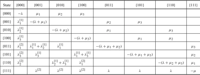
In order to describe the basic multiple dispatch hypercube model, we consider once again our system with three atoms connected by a one-way ring road (Fig. 1) with identical servers and preference matrix of Table 2. However, now we assume that in each atom j, calls can be of two types: type 1 calls (with arrival rateλ[j1]) that require the dispatch of only one unit, and type 2 calls (with arrival rateλ[j2]) that require the simultaneous response of two units. The total arrival rate of the system is:
λ=λ[11]+λ1[2]+λ[21]+λ2[2]+λ3[1]+λ[32];
the total arrival rate of type 1 calls is:λ[1]=P jλ
[1]
j , and the total arrival rate of type 2 calls is: λ[2]=P
jλ [2]
j .
are sent simultaneously; if one of them is busy, the third preferential is dispatched. When only one of the three preferential servers is available, it is assigned as a single dispatch. For both type 1 and type 2 calls, if all servers are busy, the call is lost to the system. Examples of this multi-dispatch ESS in practice are the police patrol systems studied in Chelst & Barlach (1981).
Regarding the service process, type 1 calls are serviced by a single unitiwith mean service rate µi, whereas type 2 calls are serviced by two unitsi andk, operating independently with mean service ratesµiandµk, respectively. Consequently, the model considers the two units servicing the same type 2 call as the same as two units servicing two separated type 1 calls.
The new detail observed in building the set of flow-balancing equations with respect to the toy-models of Section 2 is that: two servers become busy in the same upward transition when a type 2 call arrives and they correspond to the two highest ranked units available in the atoms server preference list. Moreover, a single server becomes busy in a transition if a type 1 call arrives at the system and this server is the first or next backup available, as well as if a type 2 call arrives at the system and the server is the only unit available in the preference list. Consequently, note that some upward transitions can occur on the diagonals of the cube representing the toy-model in Figure 2, rather than just transitions on the cube edges, such as:{000} → {011}, {000} → {101},
{000} → {110}, {001} → {111}, {010} → {111} and {100} → {111}.
For instance, consider once again state{011}, where both servers 1 and 2 are busy and server 3 is free. At this state, unit 3 can be dispatched to any atom to service a call as the preferential or backup server (see server preference list on Table 2), and the downward transition{000} → {011}
also needs to be included, since servers 1 and 2 become simultaneously busy with transition rate (λ[12]). Therefore, the flow equation of state{011}is:
λ+µ1+µ2P{011} =λ1[2]P{000} +λ[11]+λ2[1]P{001} +λ1[1]P{010} +µ3P{111}.
Note that the system leaves state{011}if a call arrives or a service is completed by server 1 or 2 (left hand side of equation). Conversely, in the right hand side of the equation the system enters state {011}: (i) from state{000}when a type 2 call arrives from atom 1; (ii) from state {001}
when a type 1 call arrives from atoms 1 or 2; (iii) from state {010}when a type 1 call arrives from atom 1; or (iv) when a service is completed by server 3. The full coefficient matrix of the system of equations for this toy-model (with zero line capacity and total backup) is shown in Table 15. By comparing to Table 3 of Section 2.1, we can observe that some blank cells in Table 3 are filled in Table 15 (e.g., in the first column and last line) representing the transition rates on diagonals or double dispatch (when two servers become busy simultaneously).
Table 15– Coefficient matrix of the system of equations for the multiple dispatch total backup model.
{ } { } { } { } { } { } { } { }
{ } −λ µ µ µ
{ } λ[ ] −(λ+µ ) µ µ
{ } λ[ ] −(λ+µ ) µ µ
{ } λ[ ] −(λ+µ ) µ µ
{ } λ[ ] λ[ ]+λ[ ] λ[ ] −(λ+µ +µ ) µ
{ } λ[ ] λ[ ] λ[ ]+λ[ ] −(λ+µ +µ ) µ
{ } λ[ ] λ[ ]+λ[ ] λ[ ] −(λ+µ +µ ) µ
{ } λ[ ] λ[ ] λ[ ] λ λ λ −µ
unit is never assigned. A practical example of such a system is theSAU-Centroviascase studied in Iannoniet al.(2008, 2009). The flow equations of the system can be built in a way similar to the single partial backup model, and by taking into account multiple dispatch transitions.
For instance, for state{011}, server 3 is idle and can service only calls arriving from atoms 2 and 3, and any call arriving from atom 1 will be lost. In case of type 2 calls arriving from atoms 2 and 3, server 3 is sent as a single dispatch since it is the only server available. The flow equation of state{011}for this zero waiting line partial backup multiple dispatch model is:
λ[21]+λ[22]+λ3[1]+λ[32]+µ1+µ2P{011}
=λ[12]P{000} +λ1[1]+λ[12]+λ[21]P{001} +λ[11]+λ1[2]P{010} +µ3P{111}.
Observe on the left hand side of this flow equation that the system leaves state{011}if either a call arrives at atoms 2 and 3, or a service is completed by server 1 or 2. Moreover, observe on the right hand side that the system enters state{011}: (i) from state{000}when a type 2 call arrives from atom 1 with rateλ[12]; (ii) from state{001}when a type 1 or type 2 call arrives from atom 1 (server 2 is sent as a single dispatch to service type 2 calls, since one of the two first preferential servers is busy), or a type 1 call arrives from atom 2 (see Table 10); (iii) from state{010}when a type 1 or type 2 call arrives from atom 1; or (iv) when a service is completed by server 3. The full coefficient matrix for this toy-model (with zero line capacity and partial backup) is shown in Table 16 (compare to Table 11 of Section 2.3).
In the case of the multi-dispatch model with total backup, the loss probability is equal to the state probability of all busy servers, P{111}, whereas in the partial backup multi-dispatch, a call can be lost to the system even when there are servers available, as shown in Section 2.3. Therefore, in a multiple dispatch toy-model, we have: the loss probability of type 1 calls, Ploss[1], the loss probability of type 2 calls,Ploss[2], and the loss probability of any call,Ploss. For example, the loss probabilityPloss, considering partial backup, for the system in Figure 1 can be formulated as:
Ploss =
λ[11]+λ[12]
λ P{011} +
λ[21]+λ[22]
λ P{110} +
λ[31]+λ[32]
T U T O R IA L O N H Y P E R C U B E Q U E U E IN G MO D E L S A N D A P P L IC A T IO N S IN E ME R G E N C Y S E R V IC E { } { } { } { } { } { } { } { }
{ } −λ µ µ µ
{ } λ[ ] −(λ+µ ) µ µ
{ } λ[ ] −(λ+µ ) µ µ
{ } λ[ ] −(λ+µ ) µ µ
{ } λ[ ] λ[ ]+λ[ ] λ[ ]+λ[ ] −(λ[ ]+λ[ ]+λ[ ] µ
+λ[ ] +λ[ ]+µ +µ )
{ } λ[ ] λ[ ]+λ[ ] λ[ ]+λ[ ] −(λ[ ]+λ[ ]+λ[ ] µ
+λ[ ] +λ[ ]+µ +µ )
{ } λ[ ] λ[ ]+λ[ ] λ[ ]+λ[ ] −(λ[ ]+λ[ ]+λ[ ] µ
+λ[ ] +(λ[ ]+µ +µ
{ } λ[ ] λ[ ] λ[ ] λ[ ]+λ[ ] λ[ ]+λ[ ] λ[ ]+λ[ ] −µ
+λ[ ]+λ[ ] +λ[ ]+λ[ ] +λ[ ]+λ[ ]
Note in this equation that each term is obtained as the joint probability that the arriving call originates at atom j (type 1 or type 2) and the two preferential servers are busy (see Table 10). For example, for atom 1, a call arriving (with probability λ[11]+λ[12]λ) when servers 1 and 2 are busy (with probabilitiesP{011}andP{111}) is lost to the system. As mentioned before, in case of type 2 calls, they can be serviced by a single server (possibly with the help of another system) if just one server from its dispatch list (with two servers) is available, and they are lost if both servers are busy.
Regarding the dispatch frequencies, we can calculate other statistics in addition to the fraction of dispatches that send serveri to atom j(fi j), such as: the fraction of dispatches that send serveri to atom jto service a type 1 call(fi j[1])(considering only type 1 calls), the fraction of dispatches that send serveri to atom jto service a type 2 call(fi j[2])(considering only type 2 calls), and the fraction of dispatches that send serversi andkto atom j to service a type 2 call(f([i2,]k)j). For example, considering the zero line total backup multiple dispatch model, the dispatch frequency of server 3 to atom 2 to service a type 2 call (taking into account only type 2 calls) as a single dispatch(f32[2])is evaluated as the joint probability that the incoming type 2 call has arrived from atom 2 and server 3 is the only available one (as a result, it is sent as single dispatch):
f32[2]=(λ [2] 2 /λ
[2])P{011}
(1−Ploss[2]) , where λ
[2]=λ[2] 1 +λ
[2] 2 +λ
[2] 3 and P
[2]
loss =Ploss =P{111}.
Alternatively, the dispatch frequency of sending servers 2 and 3 to atom 2 to answer a type 2 call is evaluated as the joint probability that the incoming type 2 call arrives from atom 2 and server 2 and 3 are idle:
f(2,3)2[2] =(λ [2] 2 /λ
[2])(P{000} +P{001})
(1−Ploss[2]) .
Similarly to the single dispatch frequencies of Section 2, the sum of these measures to all type 2 dispatches yields: 3 X j=1 3 X i=1
fi j[2]+ 2
X
i=1 3
X
k=i+1 f([i2,k])j
=1.
Using the fractions of dispatches and the inter-atoms travel distance matrix in Table 1, we obtain interesting travel distance measures, such as the mean travel distance to service type 1 calls,Tˉ[1] and the mean travel distance to service type 2 calls,Tˉ[2], defined as:
ˉ
T[1]= 3
X
j=1 3
X
i=1 fi j[1]tˉi j
and
ˉ
T[2]= 3 X j=1 2 X
i=1 3
X
k=1+1
f([i2,]k)jmin(tˉi j,tˉk j)+ 3
X
i=1 fi j[2]tˉi j
wheretˉi jis the mean travel distance from the base of serverito atom jgiven in Table 1. More-over, the mean travel time to the first and to the second ambulance arriving at a given type 2 call location can be determined, respectively, as follows:
ˉ
Tf = P3
j=1
P2 i=1
P3 k=i+1 f
[2]
(i,k)j min(tˉi j,tˉk j) P3
j=1
P2 i=1
P3 k=i+1 f
[2] (i,k)j
ˉ
Ts = P3
j=1
P2 i=1
P3 k=i+1 f
[2]
(i,k)j max(tˉi j,tˉk j) P3
j=1
P2 i=1
P3 k=i+1 f
[2] (i,k)j
In order to show how some of these measures can be evaluated in this zero line toy-model (consi-dering total and partial backup), we solve the example of Section 2 withλ[11]=0.30,λ[21]=0.45, λ3[1] = 0.60,λ1[2] = 0.10,λ2[2] = 0.15,λ3[2] = 0.20 andλ = 1.80 (note now that type 2 calls correspond to 25% of the total calls in each atom), andµ1 =µ2 =µ3 =1.0. By solving the corresponding system of linear equations of the zero line capacity and multiple dispatch model with total and partial backup, we obtain the hypercube state probabilities of Table 17. Table 18 presents the workload statistics obtained by these models.
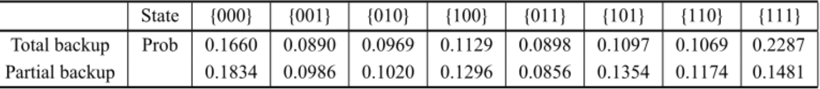
Table 17– Hypercube state probabilities for the multiple dispatch models with finite capacity queue. State {000} {001} {010} {100} {011} {101} {110} {111} Total backup Prob 0.1660 0.0890 0.0969 0.1129 0.0898 0.1097 0.1069 0.2287 Partial backup 0.1834 0.0986 0.1020 0.1296 0.0856 0.1354 0.1174 0.1481
Table 18– Server workloads for the multiple dispatch models. Serveri Workloads
Total backup Partial backup 1 0.5172 0.4676 2 0.5222 0.4531 3 0.5582 0.5305
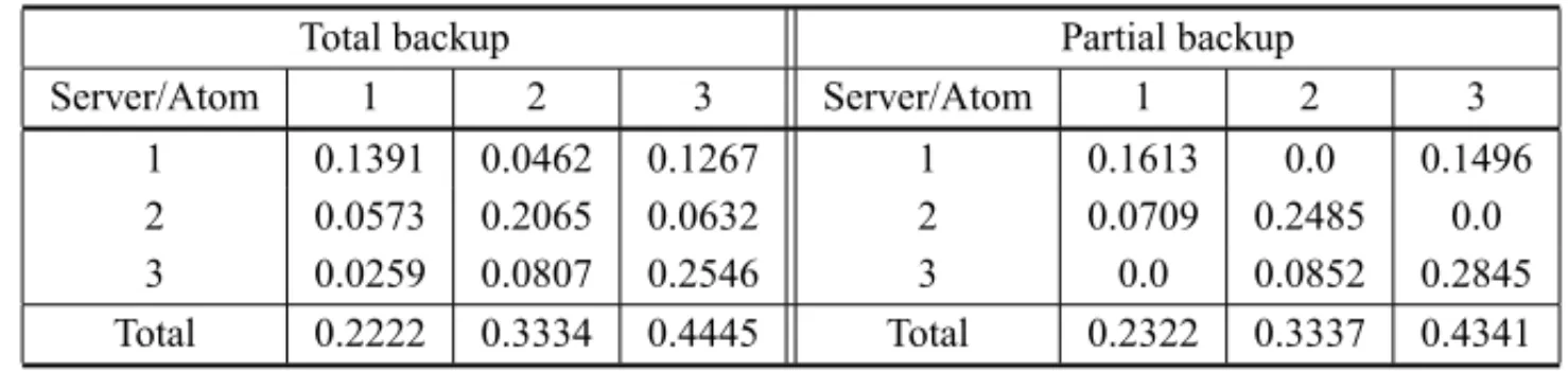
The system loss probability(Ploss)for the total backup model is 22.86%, whereas for the partial backup model, it is 26.64%. For the fraction of dispatch statistics as defined above, Table 19 presents the type 1 dispatch frequencies (fi j[1])obtained by these toy-models. Calculating the travel distance measures described above using the distance matrix of Table 1, we obtain: Tˉ[1]=
0.535,Tˉ[2]=0.535,Tˉ
f =0.220 andTˉs =1.432 for the total backup model, andTˉ[1]=0.306, ˉ
T[2]=0.306,Tˉf =0.0 andTˉs =1.0 for the partial backup model.
3.2 The model with a third state of each server
Table 19– Fraction of all type 1 dispatches that sends unitito atomj. Total backup Partial backup
Server/Atom 1 2 3 Server/Atom 1 2 3
1 0.1391 0.0462 0.1267 1 0.1613 0.0 0.1496 2 0.0573 0.2065 0.0632 2 0.0709 0.2485 0.0 3 0.0259 0.0807 0.2546 3 0.0 0.0852 0.2845 Total 0.2222 0.3334 0.4445 Total 0.2322 0.3337 0.4341
type 1 calls (single dispatch), type 2 calls (double dispatch) and type 0 “calls” (type 0 refers to locally occurring demand for service not received by the operations center, as the PIA aforemen-tioned, so that it does not involve actual calls or dispatches) with arrival rateλ[j0]. Then the total arrival rate at an atom j becomes: λj = λ[j0]+λ
[1] j +λ
[2]
j . Therefore, at a given time instant, the status of each server can be: (0) idle, (1) busy servicing a type 1 or a type 2 call, (2) busy servicing a type 0 “call”. Consequently, there are 33=27 possible states for the system.
Furthermore, the mean service rate of non-assigned calls (type 0 calls) distinguishes from the mean service rate of assigned calls (type 1 and type 2 calls), and usually there is no backup for these calls, since if the preferential server is not available when a type 0 event occurs, this call is lost to the system. Accordingly, type 0 “calls” have null travel time and no backup server, and each serveri has mean service ratesµ[I]i for types 1 and 2 calls, andµi[I I]for type 0 calls. Examples of related situations in practice are the police deployment system studied in Larson & Mcknew (1982) and the highway emergency medical system studied in Iannoni & Morabito (2007).
For instance, in building the flow balance equation to state{011}and considering total backup and the preference matrix in Table 2, we take into account that server 3 can also service type 0 “calls” at atom 3 (with rateλ[30]), and that type 0 “calls” occurring in atoms 1 and 2 are lost since servers 1 and 2 are busy. Moreover, the system can enter state{011}from state{211}when a type 0 “call” service is completed by server 3 with rateµ[I I]3 . As a result, the flow equation for the state{011}for this zero line capacity total backup model becomes:
λ−λ[10]+λ[20]+µ[I]1 +µ[I]2 P{011}
=λ[11]+λ[21]P{001} +λ1[1]P{010} +µ[I]3 P{111} +µ[I I]3 P{211}
Analyzing other states in this toy-model, for instance, state{121}where both units 1 and 3 are busy servicing a type 1 or a type 2 call, and unit 2 is busy servicing a type 0 call, we obtain the following flow equation:
µ[I]1 +µ[I I]2 +µ[I]3 P{121} =λ[32]P{020}
Observe in this equation that the system leaves state{121}if a service type 1 or type 2 is com-pleted by server 1 or server 3, or if a service type 0 is comcom-pleted by server 2, whereas the system enters state{121}: (i) from state{020}when a call type 2 arrives from atom 3 with arrival rate λ[32]; (ii) from state{021}when a call arrives in the system, except type 0 “calls” from any atom; (iii) from state{101}when a type 0 “call” arrives at atom 2, and (iv) from state{120}when a call arrives in the system, except to type 0 “calls” from any atom. Due to its size and complexity (even for a toy-model), the full coefficient matrix for this model is omitted.
Observe that the system loss probability is given by the joint probability that: (i) a type 0 call is originated at atom j, and the system is at a state in which the preferential server of atom jis busy, and (ii) a call of any type arrive at the system and all servers are busy, given by:
Ploss = λ[10]λ X
i,j,k6=0P{i j k} +λ [0] 2
λX
i,j6=0,k P{i j k} +λ[30]
λX
i6=0,j,kP{i j k} + X
i6=0,j6=0,k6=0P{i j k}.
We slightly modified the 3-server toy-model of Section 3.1, by including the type 0 “call” arrival rates and mean service times of these events. We examine an instance in which: λ[11] = 0.30, λ[21] = 0.45,λ[31] = 0.60,λ[12] = 0.10, λ2[2] = 0.15,λ[32] = 0.20,λ1[0] = 0.04,λ[20] = 0.06, λ3[0] =0.08, and the respective service rates for each unitiare: µ1[I]=µ[I]2 =µ[I]3 =1.0 and µ[I I]1 =µ[I I]2 =µ[I I3 ]=0.75. By solving the total backup zero line capacity multi dispatch toy-model with the third status discussed in this section, we computed the 27 state probabilities values in order to evaluate the mean performance measures. Table 20 presents the server workloads obtained considering the two busy status for each serveri:ρi[I]in type 1 and 2 calls andρi[I I]in type 0 calls. For instance, the expressions to evaluate these workloads to server 3 are:
ρ3[I] = P{100} +P{101} + P{102} +P{110} +P{120} +P{111} +P{112} +P{121} + P{122}
ρ3[I I] = P{200} +P{201} + P{202} +P{210} +P{220} +P{211} +P{212} +P{221} + P{222}.
Table 21 presents the type 1 dispatch frequencies by solving the total backup zero line capacity model (calculated in a similar way as the toy-models from previous sections). The system loss probability for all calls is Ploss =27.30%. In particular, for type 0 “calls” this probability is
Ploss[0] =55.93%.
Other performance measures can be computed for this system as, for example, type 2 dispatch frequencies(f([i2,k])j),i.e., the fraction of dispatches sending two serversi andksimultaneously (where unitiis the first ranked available server preference of atom jbetweeniandk): f(1,2)1[2] =
Table 20 – Server workloads for the zero line capacity multi dispatch total backup model.
Serveri Workloads
ρi[I] ρi[II] 1 0.5114 0.0247 2 0.5084 0.0364 3 0.5371 0.0446
Table 21– Fraction of all type 1 dispatches that sends unitito atomj.
Server/Atom 1 2 3
1 0.1364 0.0497 0.1318 2 0.0585 0.2008 0.0666 3 0.0272 0.0828 0.2461 Total 0.2221 0.3334 0.4445
3.3 The model with differentiated servers
In this last toy-model, we investigate a zero line capacity multiple dispatch partial backup mo-del, where the servers can be of different types. As mentioned before, there are several ESS operating with differentiated servers. For example, in some urban emergency medical systems, the ambulances can be either advanced support vehicles or basic support vehicles (case study of SAMU-Campinasin Takedaet al., 2007). Furthermore, in some systems on urban areas and on highways, the dispatch policies involve ambulances and medical vehicles – the medical vehicle is smaller and faster, but it cannot transport patients (case study ofSAU-Centroviasin Iannoni & Morabito (2007). There are other ESS in which single or multi dispatches of differentiated ser-vers occur in accordance with the type of event in common, such as vehicles and equipment for fire control services (Swersey, 1994). Consider that in our 3-servers system in Figure 1, server 1 is distinct from servers 2 and 3, since it involves other type of personnel and equipment. Assume that each atom is the home location of a server, and that we have partial backup dispatches accor-ding to the type of call and type of servers required. Thus, server 2 and 3 cannot be the backup of server 1. Consequently, in this modified version of the multiple dispatch model, calls in each atom of the system can be of 5 types, instead of only 2 types as in the basic model in Section 3.1:
– Type 1a calls (with arrival rateλ[j1a]): calls that require server 1 only. If server 1 is busy, the call is lost since server 2 or 3 is not dispatched as backup.
– Type 2a calls (with arrival rateλ[j2a]): calls that require the double dispatch of two distinct servers, server 1 and server 2 or server 3 (the first of the two available in the atom prefe-rence list). In the dispatch prefeprefe-rence list, for these calls there are three candidate servers (server 1 as first preference and servers 2 and 3 as second or third preferences). In this case, if server 1 is busy and the second preference is idle (servers 2 or 3), the former is sent as single dispatch even if the third preference is also idle, since servers 2 or 3 cannot replace server 1 (they are never assigned together to a type 2a call). However, the third preference can be sent with server 1 in case the second preference is busy.
– Type 2b calls (with arrival rateλ[j2b]): calls requiring the double dispatch of identical servers (servers 2 or 3). In this case, server 1 is never dispatched. Moreover, similar to type 2 calls of the toy-model of Section 3.1, there are two candidate servers. If only one is idle, it is sent as a single dispatch, whenever the backup unit is also busy, the call is lost.
– Type 3a calls (with arrival rateλ[j3a]): calls requiring the triple dispatch, involving servers 1, 2 and 3. However, when two or only one of them is available, a double or even a single dispatch may be assigned to such calls. If the three servers are busy, the call is lost.
The total arrival rate from atom j is defined as: λj =λ[j1]+λ[j2]+λ[j3], whereλ[j1] =λ[j1a]+ λ[j1b], λ[j2] =λ[j2a]+λ[j2b], andλ[j3] =λ[j3a]are, respectively, the arrival rates of calls requiring single (type 1 calls), double (type 2 calls) and triple (type 3 calls) dispatches to atom j. Similarly to the basic model in Section 3.1, type 1 calls are serviced by a single serveriwith a mean service rateµi. Type 2 calls are serviced by two serversiandk, which operate independently with mean service ratesµiandµk, respectively, whereas type 3 calls are serviced by three serversi,k, and l, which operate independently, with mean service ratesµi,µkandµl, respectively.
In order to model the dispatch policy, we use separate dispatch preference lists for each type of call, splitting each atom into sub-atoms A and B. This procedure is referred to aslayering (Larson & Odoni, 1981; Takedaet al., 2007, Iannoni & Morabito, 2007). Therefore, each atom j is divided into two layers: layer A (sub-atom j A) for type 1a, 2a and 3a calls serviced by distinct servers (1, 2, 3); and layer B (sub-atom j B) for type 1b, 2b calls serviced by identical servers (2 and 3). The original three atoms system is analyzed as a six sub-atoms system. The corresponding dispatch matrix is shown in Table 22.
Table 22– Server preference list (multi dispatch with differentiated servers). Atoms Sub-atoms Types of call 1stserver 2ndserver 3rdserver
1 1A 1a, 2a, 3a 1 2 3
1B 1b, 2b 2 3
2 2A 1a, 2a, 3a 1 2 3
2B 1b, 2b 2 3
3 3A 1a, 2a, 3a 1 3 2
Consider once again the state{011}and the dispatch preferences in Table 22. The system leaves this state when a call arrives, except calls type 1a from atoms 1 (1A), 2 (2A) and 3 (3A) that may be lost to the system, given that server 1 is busy and it is the only server that can service this type of call. Conversely, the system enters state{011}: (i) from state{000}when a type 2a call arrives from atoms 1 or 2 requiring the double dispatch of distinct servers 1 and 2; (ii) from state{001}
when a type 1b call arrives from atoms 1 or 2, requiring a single dispatch and server 2 is sent; or when a type 2a call arrives from atoms 1 or 2, requiring a double dispatch of two distinct servers (1 and 2), and, as server 1 is busy (and it cannot be replaced by server 3), server 2 goes to the call location as single; (iii) from{010}when a type 1a call arrives from atoms 1, 2 or 3 (single dispatch of server 1); and (iv) from state{111}when server 3 completes service. Hence, the flow equation around state{011}is:
λ− λ11a+λ12a+λ31a+µ1+µ2P{011}
= λ[12a]+λ2[2a]P{000} + λ[11b]+λ[12a]+λ[21b]+λ[22a]P{001}
+λ11a+λ12a+λ13a
P{010} +µ3P{111}.
The full coefficient matrix for this model is shown in Table 23.
As one would expect, the multi dispatch model with distinct servers and different types of calls provides additional performance statistics than the multi dispatch models presented in Sections 3.1 and 3.2. Most of these performance measures are described in details in Iannoni & Morabito (2007). For example, we may have: the loss probability of any call(Ploss)and the loss probability of each type of call (e.g., the loss probability of typemcall(Ploss[m]),m=0,1 (1a and 1b), 2 (2a and 2b), 3 (3a)). We can also obtain several frequency statistics, according to the type of call in the system, such as: single dispatch frequencies to type 1 calls (types 1a and 1b); double dispatch frequencies to type 2 calls (types 2a and 2b); double dispatch frequencies to type 3 calls (when one of the three candidate servers is busy); single dispatch frequencies to type 2b calls (when one of the two candidates servers is busy) and to type 2a and 3 calls (when two of the three candidates servers are busy), triple dispatch frequencies to type 3 calls; and the fraction of all types of dispatches from serverito atom j(fi j).
In order to show some results for this model, let us consider once again the toy-model with 3-servers of Figure 1, where now the arrival rates to each type of call (preserving the total arrival rateλ=1.80) is given by Table 24, and the mean service rates are:µ1=µ2=µ3=1.0.
The state equilibrium probabilities of this system are shown in Table 25. By using these pro-babilities we can calculate all the other measures, for example the workload for each serveri, is:ρ1=0.2994,ρ2 =0.5494,ρ3=0.5356. The system loss probability for any call(Ploss)is 31.75%; for type 1 calls(Ploss[1])the loss probability is 33.53%; for type 2 calls(Ploss[2])is 27.20%; and for type 3 calls(Ploss[3])is 11.55%.
Calculating dispatch frequencies statistics in a similar way to Section 3.1, we find the type 1 dispatch frequencies(fi j[1])presented in Table 26 (whereP3
i=1
P3 j=1 f
[1]
T U T O R IA L O N H Y P E R C U B E Q U E U E IN G MO D E L S A N D A P P L IC A T IO N S IN E ME R G E N C Y S E R V IC E { } { } { } { } { } { } { } { }
{ } −λ µ µ µ
{ } λ[ ]+λ[ ] −λ− λ[ ] µ µ
+λ[ ] +λ[ ]+λ[ ]
+µ
{ } λ[ ]+λ[ ] −(µ +λ) µ µ
{ } λ[ ] −(µ +λ) µ µ
{ } λ[ ]+λ[ ] λ[ ]+λ[ ] λ[ ]+λ[ ] −λ− λ[ ]
+λ[ ]+λ[ ] +λ[ ] +λ[ ]+λ[ ] µ
+µ +µ
{ } λ[ ] λ[ ]+λ[ ] λ[ ]+λ[ ] −λ− λ[ ] µ
+λ[ ] +λ[ ]+λ[ ]
+µ +µ
{ } λ[ ]+λ[ ] λ[ ]+λ[ ] λ[ ]+λ[ ] −λ− λ[ ] µ
+λ[ ] +λ[ ]+λ[ ] +λ[ ]+λ[ ] +λ[ ]+λ[ ]
+λ[ ]+λ[ ] +λ[ ]+λ[ ] +λ[ ]+λ[ ]
+λ[ ]
+µ +µ
{ } λ[ ]+λ[ ] λ[ ]+λ[ ] λ[ ]+λ[ ] λ[ ]+λ[ ] −λ− λ[ ] −λ− λ[ ] λ[ ]+λ[ ] −µ
+λ[ ] +λ[ ]+λ[ ] +λ[ ]+λ[ ] +λ[ ]+λ[ ] +λ[ ]+λ[ ]
+λ[ ]+λ[ ]
+λ[ ]
Table 24– Arrival rates each type of call for atomj.
Atoms Arrival rate Type Type 1 Type 2 Type 3 λj λ1ja, λ1jb λ2ja, λ2jb λ3ja
1 0.4 a 0.06 0.03 0.005
b 0.24 0.065
2 0.6 a 0.09 0.045 0.0075
b 0.36 0.0975
3 0.8 a 0.12 0.06 0.01
b 0.48 0.13
Table 25– Hypercube state probabilities for the multi dispatch zero line capacity model with distinct servers and partial backup.
State {000} {001} {010} {100} {011} {101} {110} {111} Prob 0.1924 0.0668 0.1446 0.1348 0.0606 0.0565 0.2287 0.1155
(just considering type 2 calls – types 2a and 2b), f([i2,]k)j. For instance, the fraction of dispatches sending serveri = 1 (distinct server) to atoms 1, 2 and 3 to service a type 2a call (as double and single dispatch) are: f(1,2)1[2] =0.0315, f(1,3)1[2] =0.0139, f(1,2)2[2] =0.0473, f(1,3)2[2] =0.0209, f(1,2)3[2] =0.0260, f(1,3)3[2] =0.0649, f11[2] =0.0220, f12[2] =0.0331 and f13[2] =0.0441 (where
P3 j=1[
P3 i=1 f
[2] i j +
P2 i=1
P3 k=i+1 f
[2]
(i,k)j] = 1)). Regarding travel distance measures, we ob-tain:Tˉ[1] =0.7515,Tˉ[2]=0.7957,Tˉf =0.6280 andTˉs =1.2009, and the region wide travel
distance aggregating all call types is:Tˉ =0.7671.
Table 26– Fraction of all type 1 dispatches that sends unitito atomjfor the multi dispatch model with distinct servers and partial backup.
Server/Atom 1 2 3
1 0.0468 0.0703 0.0937 2 0.1205 0.1808 0.1024 3 0.0549 0.0823 0.2484 Total 0.2222 0.3334 0.4445
4 CONCLUDING REMARKS
used to provide useful insights into problems of interest, but are mostly unable to directly address the complexity of real world ESS.
The application of hypercube family models to analyze real world ESS are promising since they are often able to capture the dispatch particularities of these systems. Some interesting ongoing and future research includes the extension of these models to: (i) capture demand scenarios du-ring different periods of the day or week of the ESS; (ii) represent priority disciplines to service queued calls; (iii) represent the re-dispatching of servers when the server can be dispatched du-ring the trip back to its base; (iv) include travel time distributions in analyzing ESS where the travel times are a significant portion of the service times (e.g., rural areas, highways); (v) con-sider multiple dispatch where the multiple servers are not sent simultaneously (e.g., the second server is sent later, if required); (vi) perform transient analyzes in situations where the steady-state assumption is not reasonable. Furthermore, other motivating future research would be the development of more effective approximate hypercube methods for embedding optimization pro-cedures in analyzing large-scale ESS, in which the use of the exact models is computationally prohibitive.
A APPENDIX
The probability that server 1 is the first server to become free when all servers are busy is given byP(X1=min(X1,X2,X3). By using an auxiliary random variableZ =min(X2,X3), we can write the desired probability as P(X1<Z). To obtain the distribution ofZ, we observe thatX2 andX3are independent exponential random variables with parametersµ2andµ3, respectively, so that:
P(Z >t)=P(X2>t)P(X3>t)=(e−µ2t)(e−µ3t)=e−(µ2+µ3)t
or
P(Z ≤t)=1−e−(µ2+µ3)t
It turns out that Z = min(X2,X3)has an exponential distribution with parameter(µ2+µ3). Then the desired probability can be obtained as:
P(X1<Z) =
Z ∞
x1=0 Z ∞
z=x1
(µ1e−µ1x1)(µ2+µ3)e−(µ2+µ3)zd x
1d z
P(X1<Z) =
Z ∞
x1=0
(µ1e−µ1x1)e−(µ2+µ3)x1d x1
By multiplying and dividing the integrand byµ=(µ1+µ2+µ3), we obtain:
P(X1<Z)=
µ
1 µ
Z ∞
x1=0
µe−µx1d x
1.
ACKNOWLEDGEMENTS
We would like to thank the three anonymous reviewers for their useful comments and suggesti-ons. This research was partially supported by CNPq, Brazil, and Fonds AXA pour la Recherche, France.
REFERENCES
[1] ALBINOJCC. 1994. Quantificac¸˜ao e locac¸˜ao de unidades m´oveis de atendimento de emergˆencia e interrupc¸˜oes em redes de distribuic¸˜ao de energia el´etrica: aplicac¸˜ao do Modelo Hipercubo. Disserta-tion, Universidade Federal de Santa Catarina, Florian ´opolis, Brazil.
[2] ATKINSONJB, KOVALENKOIN, KUZNETSOVN & MYKHALEVYCHKV. 2006. Heuristic solution methods for a hypercube queueing model of the deployment of emergency systems.Cybernetics and Systems Analysis,42(3): 379–391.
[3] ATKINSONJB, KOVALENKOIN, KUZNETSOVN & MYKHALEVYCHKV. 2008. A hypercube queu-eing loss model with customer-dependent service rates.European Journal of Operational Research,
191(1): 223–239.
[4] BATTAR, DOLANJM & KRISHNAMURTHYNN. 1989. The maximal expected covering location problem: Revisited.Transportation Science,23: 277–287.
[5] BRANDEAU M & LARSON RC. 1986. Extending and applying the hypercube queuing model to deploy ambulances in Boston. In: SWERSEYAJ & IGNALLEJ. (Eds). Delivery of Urban Services.
TIMS Studies in the Management Science,22: Elsevier, 121–153.
[6] BROTCORNE L, LAPORTE G & SEMET F. 2003. Ambulance location and relocation models.
European Journal of Operational Research,147: 451–63.
[7] BURWELLTH, JARVISJP & MCKNEWMA. 1993. Modeling co-located servers and dispatch ties in the hypercube model.Computers & Operations Research,20(2): 113–119.
[8] CHELSTK & BARLACHZ. 1981. Multiple unit dispatches in emergency services: models to estimate system performance.Management Science,27(12): 1390–1409.
[9] CHIYOSHI F, GALVAO˜ RD & MORABITO R. 2000. O uso do modelo hipercubo na soluc¸˜ao de problemas de localizac¸˜ao probabil´ısticos.Gest˜ao & Produc¸˜ao,7(2): 146–174.
[10] CHIYOSHIFY, GALVAO˜ RD & MORABITOR. 2001. Modelo hipercubo: an´alise e resultados para o caso de servidores n˜ao-homogˆeneos.Pesquisa Operacional,21: 199–218.
[11] CHIYOSHIFY, GALVAO˜ RD & MORABITOR. 2003. A note on solutions to the maximal expected covering location problem.Computers & Operations Research,30: 87–96.
[12] COSTA DMB. 2004. Uma metodologia iterativa para determinac¸˜ao de zonas de atendimento de servic¸os emergenciais. Dissertation, Universidade Federal de Santa Catarina, Florian ´opolis, Brazil. [13] GALVAO˜ RD, CHIYOSHI FY, ESPEJO LGA & RIVAS MPA. 2003. Soluc¸˜ao do problema de
localizac¸˜ao de m´axima disponibilidade utilizando o modelo hipercubo.Pesquisa Operacional, 23: 61–78.
[15] GALVAO˜ RD & MORABITOR. 2008. Emergency service systems: The use of the hypercube queu-eing model in the solution of probabilistic location problems.International Transactions in Operati-onal Research,15: 525–549.
[16] GEROLIMINIS N, KARLAFTIS M & SKABARDONIS A. 2009. A spatial queuing model for the emergency vehicle districting and location problem.Transportation Research B,43: 798–811. [17] GEROLIMINISN, KEPAPTSOGLOUK & KARLAFTISM. 2011. A hybrid hypercube – genetic
algo-rithm approach for deploying many emergency response mobile units in an urban network.European Journal of Operational Research,210(2): 287–300.
[18] GOLDBERGJB. 2004. Operations research models for the deployment of emergency services vehi-cles.EMS Management Journal,1(1): 20–39.
[19] HALPERNJ. 1977. The accuracy of estimates for the performance criteria in certain emergency ser-vice queueing systems.Transportation Science,11: 223–242.
[20] IANNONIAP & MORABITOR. 2007. A multiple dispatch and partial backup hypercube queuing model to analyze emergency medical systems on highways.Transportation Research E,43(6): 755– 771.
[21] IANNONIAP, MORABITOR & SAYDAMC. 2008. A hypercube queueing model embedded into a genetic algorithm for ambulance deployment on highways.Annals of Operations Research,157(1): 207–224.
[22] IANNONIAP, MORABITOR & SAYDAMC. 2009. An optimization approach for ambulance location and the districting of the response segments on highways.European Journal of Operational Research,
195: 528–542.
[23] IANNONIAP, MORABITOR & SAYDAMC. 2011. Optimization large-scale emergency medical sys-tem operations on highways using the hypercube queuing model.Socio-Economic Planning Sciences,
45: 105–117. doi:10.10.16/j.seps.2010.11.001.
[24] JARVISJP. 1985. Approximating the equilibrium behavior of multi-server loss systems.Management Science,31: 235–239.
[25] KOLESARP & SWERSEY AJ. 1986. The deployment of urban emergency units: a survey. In: Ma-nagement science and the delivery of urban services, edited by A. SWERSEY& E. INGALL.TIMS Studies in the Management Science, North-Holland, Elsevier22: 87–119.
[26] LARSON RC. 1974. A hypercube queuing model for facility location and redistricting in urban emergency services.Computers & Operations Research,1: 67–95.
[27] LARSON R & MCKNEW MA. 1982. Police patrol-initiated activities within a systems queuing model.Management Science,28(7): 759–774.
[28] LARSONRC. 2004. OR models for homeland security.OR/MS Today,31: 22–29. [29] LARSONRC & ODONIAR. 1981. Urban operations research. Prentice Hall. New Jersey.
[30] LUQUEL. 2007. Um estudo dos m´etodos de soluc¸˜ao do modelo hipercubo de filas para sistemas emergenciais de grande porte. Dissertation, Instituto Nacional de Pesquisas Espaciais, S ˜ao Jos´e dos Campos, Brazil.
[32] MARIANOVV, BOFFEYB & GALVAO˜ RD. 2009. Optimal location of multi-server congestible faci-lities operating as M/Er/m/N queues.Journal of the Operational Research Society,60: 674–684. [33] MENDONC¸AFC & MORABITOR. 2001. Analyzing emergency service ambulance deployment on
a Brazilian highway using the hypercube model.Journal of the Operation Research Society, 52: 261–268.
[34] MORABITOR, CHIYOSHIF & GALVAO˜ R. 2008. Non-homogeneous servers in emergency medi-cal systems: practimedi-cal applications using the hypercube queueing model.Socio-Economic Planning Sciences,42: 255–270.
[35] OWENSH & DASKINMS. 1998. Strategic facility location: A review.European Journal of Opera-tional Research,111: 423–447.
[36] RAJAGOPALANHK, SAYDAMC & XIAOJ. 2008. A multiperiod set covering location model for a dynamic redeployment of ambulances.Computers & Operations Research,35(3): 814–826. [37] REVELLECS. 1989. Review, extension and prediction in emergency service siting models.European
Journal of Operational Research,40: 58–69.
[38] REVELLECS & EISELTHA. 2005. Location analysis: A synthesis and survey.European Journal of Operational Research,165: 1–19.
[39] SACKSSR & GRIEFS. 1994. Orlando Police Department uses OR/MS methodology, new software to design patrol districts.OR/MS Today, Baltimore, 30–32.
[40] SAYDAM C & AYTUG H. 2003. Accurate estimation of expected coverage: revisited. Socio-Economic Planning Sciences,37: 69–80.
[41] SWERSEYAJ. 1994.Handbooks in OR/MS. Amsterdam: Elsevier Science BV,6: 151–200. [42] TAKEDARA, WIDMERJA & MORABITOR. 2007. Analysis of ambulance decentralization in urban
emergency medical service using the hypercube queueing model.Computers & Operations Research,