Pesqui. Oper. vol.24 número3

A METHODOLOGY TO FILTER TIME SERIES: APPLICATION TO MINUTE-BY-MINUTE ELECTRIC LOAD SERIES

Mayte Suarez-Farinas Rodrigo Lage de Sousa Reinaldo Castro Souza *

Electric Engineering Department

Pontifícia Univ. Católica do Rio de Janeiro (PUC-Rio) Rio de Janeiro – RJ

[email protected]

*Corresponding author/autor para quem as correspondências devem ser encaminhadas

Recebido em 11/2002; aceito em 08/2004 após 1 revisão Received November 2002; accepted August 2004 after one revision

Abstract

In this article a methodology for filtering a time series is presented, with application to high frequency series such as the minute-by-minute electric load series. The goal of this approach is to detect and substitute the irregularities of the time series that can produce distortions on the modelling stage. Outlier values are detected through a dynamic linear model and the Bayes factor tool; missing values are then interpolated with a Smoothing Cubic Spline. The performance of the proposed approach is illustrated using real data and evaluated through a series of tests where the irregularities have been simulated.

Keywords: load series; DLM model; irregularities in time series; cubic spline; Bayes factor.

Resumo

Neste artigo apresenta-se uma metodologia para a filtragem de séries temporais, com aplicação em séries de alta freqüência. Esta metodologia tem como objetivo detectar e substituir as irregularidades da série temporal que podem comprometer a etapa de modelagem. São detalhados o modelo linear

dinâmico utilizado para detectar os valores outliers e o emprego do Fator de Bayes. Na interpolação de

valores faltantes utiliza-se o Spline Cúbico Suavizado. O desempenho da metodologia proposta é

avaliado a través de vários testes onde as irregularidade foram simuladas.

Palavras-chave: série de cargas; modelo linear dinâmico; irregularidades em séries

1. Introduction

Following a worldwide trend, the Brazilian electric sector has been undergoing intense transformation over the last few years. In this new context, load forecasting for very short periods assumes vital importance, serving as a base not only for the calculation of future pricing of electric power, but also for the programming of optimum dispatch of the plants in the system carried out by the National Operator of the Electric Power System (ONS). Besides this operational use of these forecasting, they are also important in the routine short-term transactions of the pool electricity market, which, in Brazil, is under responsibility of another private body known as MAE (Wholesale Electricity Market).

Aimed at developing a profile for a computational system to forecast short-term electric load series for the ONS, the Cahora Project was created in a partnership between Cepel and PUC-Rio. This system and the implemented models are detailed in Rizzo (2001). The first great challenge in developing forecasting models was the great amount of irregularities found in the data retrieval system, described as follows.

CNOS, the ONS headquarters located in Brasilia, is responsible for the consolidation of load measurements for electric energy utilities in the Brazilian system. The readings of the measurement points arrive at the data retrieval centre by telemetry, at approximately 20-second intervals. Every minute, a recording is made of the available value in the reading. This system of data retrieval is subject to the occurrence of irregularities that can be motivated by erroneous information transmission, errors in data consolidation or unexpected load behaviour (blackout). These irregularities can mainly be described as:

x Occurrence of missing values: when there is no load-value readings during the interval of one minute.

x Occurrence of outliers: when the registered value is nonsense, outside the range of expected behaviour. This can be due, for example, to measurement failure at some point of the interchange or inherent problems in the information sending process. This category also includes real values corresponding to unexpected events, such as load failures or blackouts.

These irregularities can impair the performance of any forecasting model. Thus, before carrying through the half-hour load series modelling, a data treatment module has been developed. Using a filter for Missing Values and Outliers (FMO) these irregularities are corrected, transforming the minute by minute data recording into a statistically modelled time series, that can be aggregated to create higher periods series (for example, at half-hour intervals). The FMO has two main functions: that of detection of Outliers, declaring them to be missing values; and the interpolation of all resultant missing values. Once the values have been declared to be missing, these values must be substituted by values in conformity to the dynamics of the series, to pass on to the modelling stage. Since the system works as a daily basis operation, it will filter out the data obtained throughout the day on a minute-by-minute basis, at the end of the day.

In this article we describe the methodology implemented for outlier detection and missing value interpolation. Theoretical aspects related to the Dynamic Linear Models and Bayes factor, both used in outlier detection procedure and Smoothing Cubic Spline, commonly used to interpolation, are discussed in section 2 and 3. A Pattern Filter is presented in section 4 and the whole procedure is illustrated in section 5 using real electric load data. Finally, results obtained in the simulations carried out to evaluate the performance of the proposed methodology are presented in Section 6.

2. Detection of Irregularities

To model the dynamics of the time series, we used a Bayesian Linear Model with a discounting factor for the trend and the slope and a scale factor for the variance of the observations. Canton (1999) used a simpler model with a similar purpose but the trend components were not considered. For outlier detection, we used the Bayes factor, as described in West & Harrison (1986). Because some important discontinuities did not fit into this first implementation, such as the irregularities that will be described further ahead, some modifications to the original procedure have been made in order to detect them. Next, we briefly describe the outlier detection process, including a brief summary about the dynamic linear model setup and Kalman Filter equations.

2.1 The Dynamic Linear Model (DLM)

Given a time series Yt, the DLM is described by:

corr(Z

t t t t t t

t t t 1 t t

Y F . ~ N[0, V ]

G . ~ N[0, W ]

c

T Q Q

T T Z Z _t t,Q t)=0 (2.1)

where time t=1...,T; Yt is the vector of observations, with dimension nx1;Tt is the vector of parameters with dimension qx1 containing the non-observable components of the model (level, slope, seasonal component, etc.);Zt and Qt are independent and normally distributed random errors, uncorrelated to one another.

In the Bayesian formulation of this model the variances of the errors, given by the matrices Vt and Wt, must be specified. The problem of evolution of error variances must be solved, when we assume that they are unknown. Poleet al. (1994) and West & Harrison (1997) proposed a learning procedure for the unknown observation variances Vt, in terms of a scale factorIthat, in the case of normality, is the observation precision. The idea is to scale all variances and covariances in the updating equations of the DLM using I. The recursive equations of the Kalman Filter are still valid; however, conditional distributions of I will be normal while the marginal distributions will be t-Student with the degrees of freedom given by the corresponding marginal distribution ofI. Working with Vt=I

-1

, the model (2.1) can be rewritten as:

1

t t t t t

* 1

t t t 1 t t t

Y F . ~ N[0, ]

G . ~ N[0, W ]

c

T Q Q I

T T Z Z I (2.2)

observation decays with age. Thus, the prior variance for time instant t is calculated as a function of the posterior variance in time t-1, determined by a discount factorG0 (0 <G0d 1). The discount factor represents the amount of information lost with time as the series evolves. This is equivalent to establishing the variance of errors of the state vector as Wt=(G0

-1

-1)GtCt-1Gt, where Ct-1 is the variance of the posterior state vector. In this case, different discount factors for each component of the state vector are considered, as in Ameen & Harrison (1985). Thus, the vector of discount factor will be G=(G1,G2,…,Gn). For a 1-day long minute-to-minute load series, we consider a local linear trend model (F=[1,0], G=[1 1;0 1] and values of 0.9 and 0.8 were used for discount factors of level and trend respectively. So, 10% and 20% of level and trend information decays during each interval of time. (See Ameen & Harrison (1985) for comments about discount factor selection).

2.2 Kalman Filter

In what follows, we summarize the recursive equations of the Kalman Filter for this model. The distributions conditioned to values of I are the same as in the DLM with known variances and the marginal distributions are obtained from the former. The interested reader may find details about the dynamical model elsewhere, in particular in Poleet al. (1994) and Harrison & West (1997).

Initialization

At t=0, we assume * 1

0 0 0 0

(ș |D , ) ~ N m ,CI ª_¬ I º_¼, ( |D ) ~I ₀ G

>

@

Priors on time t

State Vector: * 1 , where R

t t 1 t t

(T | D, ) ~ N[a , RI I] t*I -1

= Rt.

Scale Factor: (It| Dt 1) ~ G [nt 1 / 2, dt 1 / 2], with mean 1/S

t-1, where St-1=dt-1/nt-1. The unconditional (on I) prior for state vector: , where R

t 1

t t 1 n t t

(T | D) ~ T [a , R ]

* *

t 1 t t t 1 t

m, R G C Gc

t=Rt*St-1. Here, at and Rt are calculated as in the known variance model, considering Wt calculated through the discount factors. Thus: at Gt G G where

is the inverse of the discount matrix.

* 1/ 2 1/ 2

1 2 n

diag( , ,..., )

G G G G 1/ 2

One-step-ahead forecasting

Conditional distribution: (YtDt1, )~N[ft,Q*t 1]

I I with ft F 'at t, Qt 1 .

* '

t t t F R F

*

The unconditional distribution (on I):

t 1 t Dt 1) ~ Tn[f , Q ]t t

(Y with Qt=St-1Q

* t-1. This result is similar to the one obtained when a known variance was considered, if we consider the expected value of prior St-1 as a point estimation for I until time t-1:

*

t t 1 t t t 1

Posterior (Update)

Scale Factor: p( |DI t 1,Y ) ~ G[n /2,d /2]t t t , where ,

e

2 *

t t 1 t t 1 t

n n 1, d d e /Qt t innovations.

State Vector: * 1

t t t t

(T D , ) ~ N[m , CI I], where m a * * t tR F e /Qt t t t

* 1 1 * * * *

t t R F F' Rt t t

I I _t/Q_t

C R

The unconditional distribution (marginal):

t t t) ~ T [m , Cn t t

T

( D , where

and S

] t

*

t t

C C S

t is the point estimation for the scale factor. Under these considerations, and taking into account that Rt=Rt*St-1, the equations can be rewritten as:

t

t t t t t t t t t t t t t

t-1 S

m a R F e /Q , C R R F F' R /Q

S

2.3 Bayes Factor

The Bayes factor concept was introduced by Jeffreys (1961), and constitutes a very useful tool for testing hypotheses and model selection. The Bayes factor is none other than the ratio between the likelihood function of the standard model (ModelS) and the likelihood of an alternative model (Model A). In the time series context it is used as a measure of the predictive capacity of the model. A thorough discussion, in the classical and bayesian context with multiple references and applications can be found in Kass & Raftery (1995).

West (1986) considers a procedure for a sequential monitoring of the model, based on the Bayes factor. This procedure, also discussed in West & Harrison (1986), continuously validates the predictive capacity of the model, under the bayesian approach. Since the objective is to develop a tool sensitive to local failure in the model, the Bayes factor concept was adapted. Let A be the alternative model and pA(Yt~Dt-1) be its predictive distribution. Then we can define:

t(k) p (y ,...,yt t k 1Dt k ) / p (y ,...,yA t t k 1 Dt k ) 1 k t

: d d (3.1)

If we consider :t(0)=1 t, we obtain a recursive equation for :t(k): :t(k) H .t :t 1(k 1) , where Ht is the Bayes factor based only on yt: Ht p (y Dt t 1) / p (yA t Dt 1).

In our case, the predictive distributions are t-Student

>

@

t 1

t t 1 n t t

Y | D ~ T f , Q . If we consider the alternative model, based on the use of “power discounting” as in Smith (1979), we will assume a diffuse predictive density, that is, with the same mean and variance Qat such that Qt = UQat. Then, the Bayes factor becomes:

t-1

t-1

t-1 n 1

2 ₂

t t n 1

t-1

2

t t-1 t

t n 1 2

2 2 t-1 t

t t

t-1 t (Y f ) n

Q n e

H

n e

(Y f ) n Qa

ª º

« » _{ª º}

¬ ¼ _«

» U

¬ ¼

ª º

« »

¬ ¼

Given an adjusted alternative, a value less than 1 and significantly small for Ht is an indication of the existence of discontinuity in the series. Ht indicates the existence of a potential outlier, but in cases of small or gradual changes, individual Bayes factors (based only on yt) may not be small enough to indicate failure in the model. Thus it is necessary to use jointly:t(k), whose small values suggest a possible change in the past. The algorithm proposed by West (1986) is summarized as follows: At time t, whatever may have previously occurred, proceed as follows:

Step 0. Select values of W > 0,U[0,1] and QIN.

Step 1. Compute in sequence quantities Lt and

A

Lt= Ht min(1,Lt-1) and At, the run-length parameter, as

1 1

1 1

1 1

ª

«_¬A _t

A t t

t

t

if L

if L

Step 2. Determine irregularities A. Assessment of St

If HttW, yt is consistent with the standard model St, go to B. If not, (Ht<W), yt is potentially an outlier; go to 3A.

B. Assessment of St, St-1, …

If LttW, the sequence of standard model is satisfactory (system controlled). Go to 3B.

Or else (Lt<W,) or (At> Q); then, we have structural breaks. Go to 3A.

Step 3. Update

A. Reject observation yt. Update Kalman Filter equation allowing for change: incrementing the uncertainty of state vector: mt= at, Ct=ĮCt

B. The sequence of standard model is satisfactory. Standard update of Kalman Filter equation.

When = 1 the discontinuity is of the “transient” type. Value > 1 indicates a structural change that started in instant t -A + 1. When > Q, even when > Q, we can admit that at instant t, a slow structural change is occurring, from instant t - + 1.

t

A At

t

A

t At

At

Considering the characteristics of the short-term load series, certain alterations to West’s algorithm had to be considered. In West’s algorithm, when we are in the presence of any type of discontinuity the update of the model must be made in such a mode as to allow for changes in the model. The variance matrix of posterior density is multiplied by a factor greater than one. This factor can be a matrix, allowing a different inflation for the posterior variance of each component. This is also advisable in the case of missing values.

This algorithm should identify outliers and structural changes. In our case, the minute-by-minute load series frequently has 2 and up to 4 consecutive outliers, without this implying a structural change. An adaptation of the model, that increased the uncertainty of the model when faced with an outlier, would make it difficult to detect other outliers later on. As our goal is not modeling but the detection of discontinuities, we propose to increase the uncertainty only when a structural change is detected, keeping the uncertainty unchanged when an outlier is detected. Furthermore, our data presents large intervals with consecutive missing values; consecutive increments to the variance matrix would make it diverge numerically, making the system unavailable for outlies detection. Thus, we decided not to increment variance in the case of missing values.

According to the nature of the data, abrupt structural changes cannot happen because the load cannot have a very strong variation from one minute to the next. Hence, both the outlier values and structural changes must be substituted. When a structural change is detected, if it is a permanent one, all the values in its neighbourhood are substituted in order to smooth the structural change.

3. Missing Values Interpolation

Some methodologies for missing values estimation in time series have been proposed the literature. Parametric alternatives have been widely used (Brubacher, S.R. et al., 1976), by means of a statistical model to adjust the data, and using it later in the interpolation. Ferreiro (1987), Harvey & Pierse (1984) and Ljung (1989) use this approach as well.

A natural idea to substitute the missing values and outliers would be to use the bayesian model adjusted in the outlier declaration stage and then to substitute the extraneous observations with the one-step-ahead forecasts made in the previous instant. However, the existence of data blocks with many consecutive missing observations (or declared outliers), sometimes for more than a one hour period (60 observations), made it necessary to abandon these techniques because, as the forecast horizon grows the forecasts cease to be reliable. Thus, we decided to use the smoothing cubic spline, previously applied to the interpolation of time series by Gordon (1996) and to the handling of missing values in Koopman (1991) and Koopmanet al. (1998).

3.1 Smoothing Cubic Spline (SCS)

The Smoothing Cubic Spline (SCS) is a non-parametric techniques that has been applied in interpolation problems in time series (see Ferreiro, 1987; and Koopmanet al., 1998) with good results. This method has been used in some packages such as the SsfPack (Koopman

et al., 1998b). However, the SCS is not well-behaved for series with a considerable number

solutions with accented curvature when many consecutive missing values are presented, distancing itself from the pattern of the data, as we will see further ahead.

The underlying idea in cubic spline is the smoothing of a third-order polynomial. This smoothing is effected through a model in state space form that represents the spline, afterwards using the Smoothing Kalman Filter (SKF), as described in Kohn & Ansley (1987). This type of model takes into consideration all the available values and not only three points.

Weinertet al. (1980) defines in a general way the concept of smoothing spline, discussing the problem and establishing the existence and uniqueness of the solutions. Kohn & Ansley (1987) discuss the particular case of polynomial splines defined as follows:

Let t1, t2... tNbe the available time periods. The problem of interpolation by smoothing polynomial splines consists of the searching of a polynomial f that minimizes the loss function:

(3.3)

^

`

^

`

N _{2 1}

2

t i ₀

i 1

Y (t ) L (t)

¦

³

where L is the differential operator L=dm/dtm. When m=2, we will have the smoothing cubic spline and the loss function consists of the integral of the square curvature, and the solution is such that Yti=f(ti).

Wahba (1978) and Weinertet al. (1980) represent the spline as the limit of the conditional expectancies of a random process. This allows Kohn & Ansley (1987), Koopman (1991) to establish efficient algorithms to adjust the smoothing cubic spline, through the recursive equations of the SKF to state space form of the random model. The reader may find a synthetic description in Durbin & Koopman (2001).

In the case where the number of consecutive missing values is not so high, spline cubic offers a good solution. But, on the other hand, when there are many consecutive missing values to interpolate, the spline does not reflect all the details of the load curve due to the softness of the solution. For this reason we propose to substitute missing values with a convex combination of cubic spline and a value which reflects the load-curve pattern. Let Yt be the minute-by-minute load series. Assume that Yt is a missing value at time t=to. This missing value will be substituted by the convex linear combination of the values SYt and TYt. That is: Yto=DTYto+(1-D)SYto, where St is the value interpolated by smoothing cubic spline and TYtis the value of the load corresponding to the same time instant of the day with the load pattern nearest to the current day pattern. Given the load curve, the procedure to find a similar stretch to interval [t-stretch, T-1] where t is the corresponding time instant and Yt is the value to substitute. The criterion used to select similar stretch could be the minimum mean square error of the average quadratic error, after adjusting both intervals to the same mean.

4. Pattern Filter

stereotyped and reproducible. The telemetry system that feeds data to CNOS may have technical or transmission problems resulting, rarely, in a large (days) batch of data which fail to conform to this stereotyped daily pattern. It has happened, for example, that the load curve of a certain day failed to match the expected pattern for that day, without any visible outliers that could cause such a deviation. To solve this problem it was decided to implement the Filter of Pattern (FP) on the aggregated series every 30 minutes.

Pattern Filter Methodology

In previous work, Sobral (1999) established a classification of hourly load curves in several types for one of the Brazilian utilities using a 4x4 Kohonen Neural Network. In this work, the days were grouped according to the hourly load pattern and the prototypes were obtained. These prototypes will serve as a base for the implementation of the Filter of Pattern.

As the idea is to compare the prototypes with the load series at 30-minute intervals, the same groups have been used. From the hourly-load profiles of each group, we have obtained through linear interpolation the profiles of the load curve at each 30-minute interval. For day d we have a 30-minute load curve and then we analyze whether it follows the expected pattern. In order to do this, we select the most adequate profile using certain criteria. We use for this selection the nearest prototype to a Mean Absolute Percentage Error (MAPE). Taking into consideration that the goal is the daily pattern and not the mean of the load, we make sure that the two curves (the daily curve and the nearest prototype) have the same mean, for the MAPE computation. If the MAPE of the nearest profile is bigger than the specified threshold, we consider this day to be outside the expected standard and substitute it.

We do not propose that the whole day should be substituted because it might be the case that not all intervals of the day are responsible for the pattern failure. Thus, the day is divided into the following intervals: 00:00h to 05:30h; 06:00h to 11:30h; 12:00h to 14:30h; 17:00h to 19:30h; 20:00h to 23:30h. With them, we detect those with a MAPE bigger than the threshold. These intervals are substituted by the corresponding intervals of the profile curve that had been adjusted to have the same mean as the curve of day under study. The threshold chosen for the MAPE was 5%. At first glance, this value may seem small but we should remember that both curves have the same mean. Furthermore, to choose this value, we observed the behaviour of this statistics for a number of days, including some days that had been considered out-of-pattern by the experts.

5. Application to Real Data

(a) (b)

Figure 5.1 – Minute-by-minute load series. Month: August (a) Original Series. (b) Outliers detected.

We then used the missing values interpolation procedure described in section 3 to substitute 348 observations (0.78%) declared missing values and outliers of the load series. The resulting series is shown in Figure 5.2 (b).

(a) (b)

Figure 5.2 – minute-by-minute load series. Month: August (a) Original Series. (b) Series having substituted outliers and missing values.

A typical case where the Pattern Filter is required is illustrated in Figure 5.3. Here we show the series for September 1999. After the missing values and outlier filter, the series was aggregated in a 30-to-30 minutes series as shown in Figure 5.3 (a). An anomaly is obvious in the period between the 13th and 20th of September (around observations 600-1000), as an abrupt decrease in the daily variance. Power engineers assure us that this decrease in the variance did not, in fact, happen. Figure 5.3 (b) shows the resultant series after pattern filtering, showing a more plausible pattern.

(a) (b)

Figure 5.3 – Aggregated 30-to-30 minute Load Series. Month: September. (a) Original Series (b) Filtered Series.

This example was meant only as a qualitative illustration that the methodology is well behaved. In the next section we shall quantitatively evaluate the performance of the procedure in a variety of situations.

6. Test and Results

6.1 Outlier Test

For this test, outliers were artificially generated in the set of times described in Table 1. In observations chosen to become outliers, the value of the real load was increased by 50%, that is, if in a specific minute the value of the load were 1000, it would be substituted by 1500. The resulting data was then passed through the outlier filter. The table containing the data where outliers were generated can be found in Annex 2 of Table A1. The filter detected all outliers generated in this fashion, for a 100% success rate.

6.2 Missing Value Tests

Two types of missing values were considered: short and long term sets.

6.2.1 Test for short-term missing values

In the original data, three 15-minute-long sequences were declared missing (i.e, their load values were set to -999.99); they appear in Table 4. The same missing-value sequences were considered for both utilities. Table A2 in Annex 2 contains data from which missing values were generated.

The MAPE of the value filled-in by the filter versus the real value for each sequence of missing values was computed for each day, for special days, and for common days, at peak hours and at normal off-hours, as well as the General MAPE. The results appear in Table 6.1.

Table 6.1 – Results of filter – short-term missing values

MAPE

South Southeast

Peak-hour demand 0.0463 0.0846

Off-hour demand 0.0595 0.0739

Special Days 0.0604 0.0842

Common Days 0.0449 0.0792

GENERAL 0.0507 0.0811

The results obtained with the application of the filter in short-term sequences can be considered good in terms of MAPE, all values being below 0.1%. For common days as well as for special days, the maximum values of this measure were under 0.118% and 0.125%, respectively for South and Southeast utilities. Average values occurred between 0.04% and 0.061% for South utility and between 0.07% and 0.085% for Southeast utility.

6.2.2 Test for long-term missing values

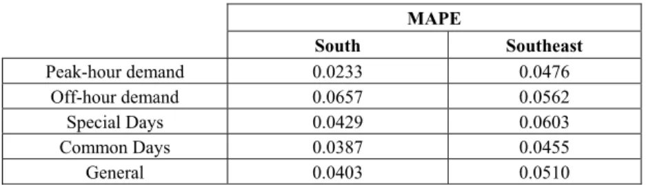
the real value was computed. These values can be found in Table 6.2. Besides the interval value, there appear values consolidated by day, by type of day and the general value as well.

Table 6.2 – Results of the filter – long-term missing values

MAPE

South Southeast

Peak-hour demand 0.0233 0.0476

Off-hour demand 0.0657 0.0562

Special Days 0.0429 0.0603

Common Days 0.0387 0.0455

General 0.0403 0.0510

The results obtained with the application of the filter continue to be good when long-term sequences are considered. Both for weekdays as well as for holidays, the maximum values for this measure were under 0.062% and 0.105%, respectively, for South and Southeast. Average values remained between 0.023% and 0.066% for South utility and between 0.045% and 0.061% for Southeast utility. Values for peak-hour demand were slightly better but the length of the sequence was smaller than in the off–hour demand period.

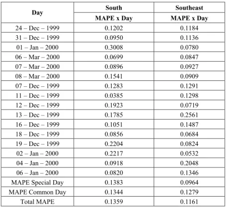
6.3 Test for Pattern Filtering

The data used for this test were previously filtered and added in a thirty-to-thirty minute series. Thus, these data do not present any other type of irregularity. To introduce an irregularity into the load standard, each day was substituted by its average, so that this day had an unexpectedly low standard deviation. The MAPE of the values filled by the filter in relation to the real values were computed. The procedures for attainment of the profiles of the daily curve of Southeast and South utilities are detailed in Annex 1.

The results obtained through the application of the PF in 30-by-30-minute sequences turned out well. Both for common days as well as for special days, the maximum values of this measure were under 0.3% and 0.26%, respectively, for South and Southeast utilities. Average values were placed between 0.14% and 0.13% for South and between 0.096% and 0.128% for Southeast utility.

7. Conclusions

Table 6.3 – Results of Pattern Test Utilities

South Southeast Day

MAPE x Day MAPE x Day

24 – Dec – 1999 0.1202 0.1184

31 – Dec – 1999 0.0950 0.1136

01 – Jan – 2000 0.3008 0.0780

06 – Mar – 2000 0.0699 0.0847

07 – Mar – 2000 0.0896 0.0927

08 – Mar – 2000 0.1541 0.0909

07 – Dec – 1999 0.1283 0.1291

11 – Dec – 1999 0.0385 0.1298

12 – Dec – 1999 0.1923 0.0719

13 – Dec – 1999 0.1785 0.2561

16 – Dec – 1999 0.1051 0.1487

18 – Dec – 1999 0.0856 0.0684

19 – Dec – 1999 0.2204 0.0824

02 – Jan – 2000 0.2217 0.0532

04 – Jan – 2000 0.0918 0.2048

06 – Jan – 2000 0.0820 0.1346

MAPE Special Day 0.1383 0.0964

MAPE Common Day 0.1344 0.1279

Total MAPE 0.1359 0.1161

Acknowledgments

The authors would like to thank Sandra Canton for discussion of the ideas of this paper, Lucio de Medeiros and anonymous referees for their comments on the original draft of the paper, Marcelo Magnasco for the carefully revision of the manuscript and CNPq for financial support.

References

(1) Ameen, J.R.M. & Harrison, P.J. (1985). Normal Discount Bayesian Models (with discussion).In:Bayesian Statistics 2 [edited by J.M. Bernardoet al.], North Holland, Amsterdam, 271-298.

(2) Brubacher, S.R. & Tunnicliffe Wilson, G. (1976). Interpolating Times Series with Application to the estimation of holiday Effects on electricity. Applied Statistic,25(2), 107-117.

(4) Durbin, K. & Koopman, S.J. (2001). Time Series Analysis by State Space Models.

Oxford, New York.

(5) Ferreiro, O. (1987). Methodologies for the estimation of missing observations in time series.Statistics and Probability Letters,5, 565-69.

(6) Gordon, F. (1996). Previsão de carga diária através de modelos estruturais usando splines. Doctoral Thesis, DEE/PUC-Rio.

(7) Harrison, P.J. (1965). Short term sales forecasting. Applied Statistics,15, 102-139. (8) Harvey, A.C. & Pierse, R. (1984). Estimating missing observation in the economic time

series.Journal of American Statistical Association,79(385), 125-131.

(9) Jeffreys, H.J. (1961). Theory of Probability. Third Edition. Clarendon Press, Oxford. (10) Kohn, R. & Ansley, C.F. (1987). A New algorithm for spline smoothing based on

smoothing a stochastic process. SIAM J Sci Statistical Computing,8, 33-48.

(11) Koopman, S.J.; Shephard, N. & Doornik, J.A. (1998). Statistical algorithms for models in state space using Ssf Pack 2.2. Econometrics Journal,1, 1-55.

(12) Koopman, S.J. (1991). Efficient smoothing algorithms for time series models. Doctoral Thesis.

(13) Koopman, S.J.; Shephard, N. & Doornik, J.A. (1998b). SsfPack 2.0: Statistical algorithms for models in state space. AnOx link to underlying C code. Available on website: cwis.kub.nl/~fews/center/staff/koopman/SsfPack.htm.

(14) Ljung, G.M. (1989). A note on the estimation of missing values in time series.

Commun. Statist. – Simula.,18(2), 459-465.

(15) Pole, A.; West, M. & Harrison, J. (1994). Applied Bayesian Forecasting and Time

Series Analysis. Chapman & Hall, New York.

(16) Kass, R. & Raftery, A.E. (1995). Bayes factors. Journals of the American Statistical Association,90, 773-795.

(17) Rizzo, G.M. (2001). Previsão de Carga de Curtíssimo Prazo no Novo Cenário Elétrico Brasileiro. Master’s Degree Dissertation, DEE, PUC-Rio.

(18) Sobral, A. (1999). Modelo de previsão horária de carga elétrica para Light. Master’s Degree Dissertation, DEE, PUC-Rio.

(19) Wahba, G. (1978). Improper priors, spline smoothing and the problem of guarding against model errors in regression. J. Roy. Statist. Soc. Ser. B,40, 584-589.

(20) Weinert, H.L.; Byrd, R.H. & Sidhu, G.S. (1980). A stochastic framework for recursive computation of spline functions: part II, Smoothing splines. J. Optim. Theory Appl.,30, 255-268.

(21) West, M. & Harrison, J. (1989). Bayesian Forecasting and Dinamic Models. Springer-Verlag, New York.

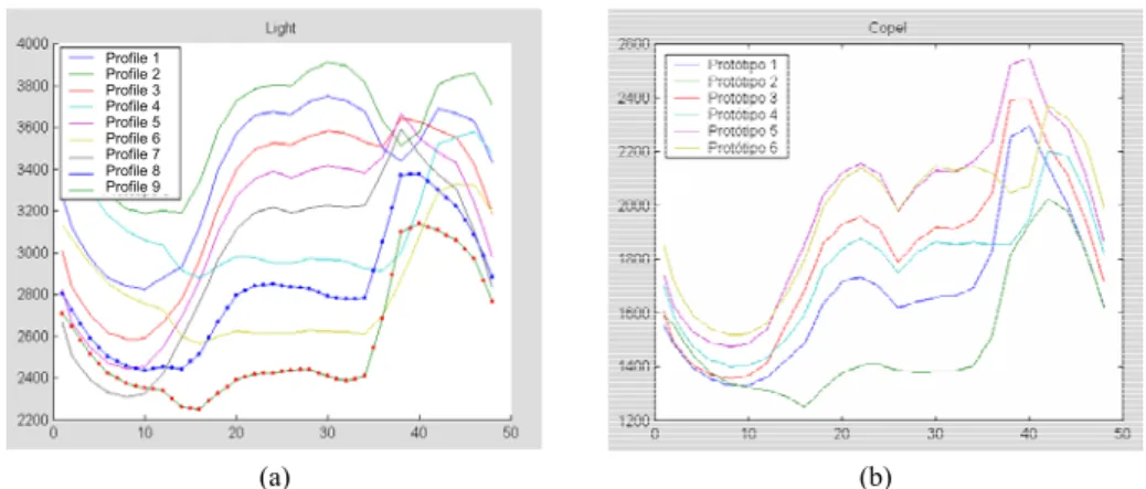
Appendix 1 – Load Profiles for Southeast and South Utilities

The Load profiles used as base for the filter of standards was estimated by Sobral (1999) who used a neural network argument (Kohonen classification) to derive the different profiles for both utilities. The Kohonen algorithm produces 9 and 6 distinct profiles, respectively, for the two utilities being analyzed, as shown below in Figure 9. For more details, the reader is referred to Sobral (1999).

Profile 1 Profile 2 Profile 3 Profile 4 Profile 5 Profile 6 Profile 7 Profile 8 Profile 9 Profile 1 Profile 2 Profile 3 Profile 4 Profile 5 Profile 6 Profile 7 Profile 8 Profile 9

(a) (b)

Figure 9 – 30-to-30-minute-load-curve profiles. a) Southeast utility b) South utility.

Appendix 2 – Observations Used in the Simulation

Table A1 – Observations that generated outliers

Type of Day Year Day Day of the Week Hours

24 – Dec Special Day 06:00; 15:00; 19:00 1999

31 – Dec Special Day 06:10; 15:10; 19:10 01 – Jan Holiday 06:20; 15:20; 19:20 06 – Mar Carnival 06:30; 15:30; 19:30 07 – Mar Carnival 06:40; 15:40; 19:40 Day of Special

Event or

holiday ₂₀₀₀

08 – Mar Carnival 06:50; 15:50; 19:50 07 – Dec Tuesday 07:00; 16:00; 20:00 11 – Dec Saturday 07:10; 16:10; 20:10 12 – Dec Sunday 07:20; 16:20; 20:20 13 – Dec Monday 07:30; 16:30; 19:30 16 – Dec Thursday 07:40; 16:40; 20:40 18 – Dec Saturday 07:50; 16:50; 20:50 1999

19 – Dec Sunday 08:00; 17:00; 21:00 02 – Jan Sunday 08:10; 17:10; 21:10 04 – Jan Tuesday 08:20; 17:20; 21:20 Normal Day

2000

Table A2 – Short-termmissing values sequence

Type of

Day Year Day

Day of the

Week Hours

24 – Dec Special Day 05:30 to 05:44; 14:30 to 14:44; 18:30 to 18:44 1999

31 – Dec Special Day 05:35 to 05:59; 14:35 to 14:49; 18:35 to 18:59 01 – Jan Holiday 05:40 to 05:54; 14:40 to 14:54; 18:40 to 18:54 06 – Mar Carnival 05:45 to 05:59; 14:45 to 14:59; 18:45 to 18:59 07 – Mar Carnival 05:50 to 06:04; 14:50 to 15:04; 18:50 to 19:04 Day of

Special Event or

Holiday 2000

08 – Mar Carnival 05:55 to 06:09; 14:55 to 15:09; 18:55 to 19:09 07 – Dec Tuesday 06:00 to 06:14; 15:00 to 15:14; 19:00 to 19:14 11 – Dec Saturday 06:05 to 06:19; 15:05 to 15:19; 19:05 to 19:19 12 – Dec Sunday 06:10 to 06:24; 15:10 to 15:24; 19:10 to 19:24 13 – Dec Monday 06:15 to 06:29; 15:15 to 15:29; 19:15 to 19:29 16 – Dec Thursday 06:20 to 06:34; 15:20 to 15:34; 19:20 to 19:34 18 – Dec Saturday 06:25 to 06:39; 15:25 to 15:39; 19:25 to 19:39 1999

19 – Dec Sunday 06:30 to 06:44; 15:30 to 15:44; 19:30 to 19:44 02 – Jan Sunday 06:35 to 06:49; 15:35 to 15:49; 19:35 to 19:49 04 – Jan Tuesday 06:40 to 06:54; 15:40 to 15:54; 19:40 to 19:54 Normal

Day

2000