AN ADD/DROP PROCEDURE FOR THE CAPACITATED PLANT LOCATION PROBLEM
Claudio Thomas Bornstein *
Engenharia de Sistemas e Computação / COPPE Universidade Federal do Rio de Janeiro
Rio de Janeiro – RJ [email protected]
Manoel Campêlo
Departamento de Estatística e Matemática Aplicada Universidade Federal do Ceará
Fortaleza – CE
* Corresponding author / autor para quem as correspondências devem ser encaminhadas
Recebido em 06/2003; aceito em 10/2003 Received June 2003; accepted October 2003
Abstract
The capacitated plant location problem with linear transportation costs is considered. Exact rules and heuristics are presented for opening or closing of facilities. A heuristic algorithm based on ADD/DROP strategies is proposed. Procedures are implemented with the help of lower and upper bounds using Lagrangean relaxation. Computational results are presented and comparisons with other algorithms are made.
Keywords: capacitated plant location problem; ADD/DROP procedures; heuristic methods; Lagrangean relaxation.
Resumo
O problema de localização de facilidades capacitado com custos de transporte lineares é considerado. Testes exatos e heurísticas para abrir ou fechar facilidades são apresentados. Um algoritmo heurístico baseado em estratégias ADD/DROP é proposto. Os procedimentos são implementados com o auxílio de limites inferiores e superiores provenientes de relaxação lagrangeana. Resultados computacionais são apresentados e comparações realizadas com outros algoritmos.
1. Introduction
The capacitated plant location problem (CPLP) may be formulated as:
minimize kj kj k k
k I j J k I c x f y
∈ ∈ ∈
+
∑ ∑
∑
subject to kj k k
j J
x a y k I
∈
≤ ∀ ∈
∑
kj j k I
x b j J
∈
= ∀ ∈
∑
0 ,
kj
x ≥ ∀ ∈ ∀ ∈k I j J
{0,1}
k
y ∈ ∀ ∈k I
where I is the set of possible plant locations each with a maximum capacity ak and fixed cost
fk, J is the set of demand centers each with a demand bj, and ckj is the unit transportation cost
between a facility k and a consumer j. The variable xkj represents the amount sent from k to j,
and yk means locating (or not) plant k.
The CPLP is a well known combinatorial optimization problem belonging to the class of the NP-Hard problems. For large instances there may be the need of reduction tests, problem relaxation and heuristic methods. Christofides & Beasley (1983), Beasley (1988) and Barcelo et al. (1991) have used problem reduction and Lagrangean relaxation to solve the CPLP. Thizy (1994) has used Lagrangean relaxation for a variant of the CPLP. Beasley (1993) has developed a framework for producing Lagrangean heuristics for the capacitated and the uncapacitated plant location problems. A good comparison of heuristic methods for the CPLP is presented by Cornuejols et al. (1991).
Here we present a heuristic algorithm for the CPLP based on dominance criteria between fixed and variable costs. These criteria may work in an exact way or just as a heuristic method for determining the status of facilities. Jacobsen (1983) and Mateus & Bornstein (1991) have used them within ADD or DROP heuristics. Holmberg & Ling (1995) have applied an ADD heuristic for the CPLP with staircase costs. More recently Bornstein & Azlan (1998) have used these ideas within the simulated annealing framework.
In the next section we present reduction tests and heuristics based on dominance criteria. The tests and heuristics are well known from literature. However, we combine them in a new way producing the algorithm proposed in section 3. We use lower and upper bounds for the cost increments in order to get an efficient implementation. These bounds can be obtained by Lagrangean relaxation (see Azlan, 1995).
In section 4 we present computational results. A comparison with other known algorithms is made. Finally, the last section points out to some conclusions.
2. Dominance Criteria
Given a subset K⊆Iof the potential plant locations, let
( ) min kj kj ( )
k K j J
w K c x x X K
∈ ∈
= ∈
∑ ∑
represent the solution value of the transportation problem T(K) associated with the CPLP, where
( ) [ kj] kj k, ; kj j, ; 0,kj ,
j J k K
X K x x x a k K x b j J x k K j J
∈ ∈
= = ≤ ∀ ∈ = ∀ ∈ ≥ ∀ ∈ ∀ ∈
∑
∑
.If X K( )= ∅, we consider w K( )= +∞.
The function w( ) has the important property of supermodularity (Proposition 10 in Wolsey, 1983). A function w( ) is said to be supermodular (or equivalently −w( ) submodular) if
( ) ( ) ( ) ( )
w K −w K∪ ≤i w K′ −w K′∪i ∀K′⊆K and ∀ ∉i K (see Wolsey, 1983 and
Nemhauser & Wolsey, 1988). Thus, supermodularity is a kind of concavity.
For i∈ −I K let δi( )K =w K( )−w K( ∪ ≥i) 0 evaluate the increase/decrease in transportation costs if we close/open facility i. Furthermore, let ∆i( )K = fi−δi( )K evaluate the balance between fixed and variable costs with respect to facility i. The function ∆i( ) gives rise to criteria for opening or closing plant i.
Let K0 and K1 be the sets of closed and opened plants, i.e., K0= ∈{i I |yi =0} and
1 { | i 1}
K = ∈i I y = . Facilities whose status is still undefined remain in K2= −I K0−K1. We can state the following rules (see Akinc & Khumawala, 1977 and Mateus & Bornstein, 1991):
Add-test: If ∆i(K1∪K2− ≤i) 0 then yi =1. Drop-test: If ∆i(K1)≥0 then yi=0.
Starting with K0 =K1= ∅ we begin using the Add-test, assigning plants to K1. If K1 is
big enough (X K( 1)≠ ∅), allowing the evaluation of ∆i(K1), we may use the Drop-test, allocating plants to K0. The optimality of the decision is assured by supermodularity of w( ).
Increasing set K0 decreases set K1∪K2 leading to non-increasing values of
1 2
( )
i K K i
∆ ∪ − . Similarly, increasing K1 yields non-decreasing values of ∆i(K1).
The following figure illustrates how the Add- and Drop- tests work. The arrows show how
1
( )
i K
∆ and ∆i(K1∪K2−i) move while the tests are used.
→ ←
1
( )
i K
∆ ∆i(K1∪K2−i)
(
1]
If we get K2 ={ }i then ∆i(K1)= ∆i(K1∪K2−i), closing the gap
[
∆i(K1),∆i(K1∪K2−i)]
,meaning that the use of the Add- and Drop- tests leads to an optimal solution of the CPLP. Unfortunately this seldom happens. There is usually a situation where
1 1 2 2
( ) 0 ( )
i K i K K i i K
∆ < < ∆ ∪ − ∀ ∈ . In order to proceed, the following heuristics may be used (see Jacobsen, 1983):
Add-heuristic: If ∆i(K1)<0 then yi=1
Drop-heuristic: If ∆i(K1∪K2− >i) 0 then yi=0
Now supermodularity does not guarantee optimality anymore. Moreover, for a plant i
satisfying ∆i(K1)< < ∆0 i(K1∪K2−i) the rules above allow both yi=0 and yi=1.
Trying to escape from this dilemma we look for a plant giving min (∆i K1) or
1 2
max (∆i K ∪K −i). The former seems to be the best one to be opened whereas the latter seems to be the most advantageous one to be closed.
One of the difficulties with the Add- and Drop- tests and heuristics is the requirement of solving a great number of transportation problems, which may be very time consuming. The use of approximations for ∆i( ) is an alternative for efficient implementation. Using the dual solutions of problems T K( 1∪K2) and T K( 1), Azlan (1995) applies Lagrangean relaxation to calculate lower bounds wL(K1∪K2−i) and wL(K1∪i). Thus, upper and lower bounds
1 2
( )
U
i K K i
∆ ∪ − and ∆Li(K1) are obtained (see also Bornstein & Azlan, 1998).
3. The Algorithm
The algorithm uses the dominance criteria studied in the previous section. It starts with
0 1
K =K = ∅ and K2=I and repeatedly applies the tests and heuristics defined above. The
algorithm consists of two phases. Phase 1 defines the status of all plants, ending with
2
K = ∅. Plants are assigned to K1, K0 and K0, where K0 is the set of temporarily closed plants. Phase 2 refines the solution reexamining the plants placed in K0. The number of plants assigned to K0 depends on a parameter ε. Smaller values of ε result in a greater number of plants to be only temporarily closed.
Phase 1 begins with the Add-test being used at step 2. Facilities still remaining in K2 have
1 2
( ) 0
U
i K K i
∆ ∪ − > leading to the use of the Drop-heuristic. At step 4 facility s with
maximum ∆Ui (K1∪K2−i) is chosen. For greater accuracy the exact value ∆s(K1∪K2−s) is calculated at step 5 and examined at step 6. If ∆s(K1∪K2− ≤s) 0 (this is possible
because now we consider the exact value) then we open facility s. If
1 2
0< ∆s(K ∪K − ≤s) fs(1−ε), where 0≤ <ε 1, then we put s in K0. Finally if
1 2
(1 ) ( )
s s
PHASE 1
Step 0: (* Initialization *)
2 1 0 0
1 2
Set and . Choose 0 <1
Calculate ( )
K I K K K
w K K
ε
= = = = ∅ ≤
∪
Step 1: (* Calculating approximations for K2*)
1 2 1 2 1 2 2
Calculate (δiL K ∪K − =i) wL(K ∪K − −i) w K( ∪K ) ∀ ∈i K
1 2 1 2 2
( ) ( )
U L
i K K i fi δi K K i i K
∆ ∪ − = − ∪ − ∀ ∈
Step 2: (* Choosing plants to be opened *)
{
2 1 2}
1 1 2 2Set A= ∈i K |∆Ui (K ∪K − ≤i) 0 , K =K ∪A and K =K −A
Step 3: (* Phase 2? *)
2
If K = ∅, Phase 2!
Step 4: (* Choosing plant s *)
{
}
2
1 2 1 2
( ) max ( )
U U
s K K s i K∈ i K K i
∆ ∪ − = ∆ ∪ −
Step 5: (* Calculating exact values for plant s *)
1 2
1 2 1 2 1 2
Calculate ( )
( ) ( ) ( )
s s
w K K s
K K s f w K K s w K K
∪ −
∆ ∪ − = − ∪ − + ∪
Step 6: (* Defining status of plant s *)
2 2
1 2 1 1
1 2 0 0 0 0
{ }
If ( ) 0 then { } and go to step 3
If ( ) (1 ) then { } else { }
Go to step 1
s
s s
K K s
K K s K K s
K K s f ε K K s K K s
= −
∆ ∪ − ≤ = ∪
∆ ∪ − ≤ − = ∪ = ∪
The convergence of phase 1 can be shown very easily. There are two loops. The first consists of steps 1 to 6 and the second consists of steps 3 to 6. At each iteration of phase 1 one of the two loops is executed and a facility is discarded from set K2 at step 6. This finishes
emptying set K2 leading to phase 2.
Phase 2 uses the Add-heuristic meaning the evaluation of ∆i(K1) or its lower bound
1
( )
L i K
∆ . Therefore we need K1 big enough to guarantee X K( 1)≠ ∅. Let us show that
this will always happen at the end of phase 1. One should just consider that at step 6 an element s will only be removed from K1∪K2 if ∆s(K1∪K2− >s) 0. This means
1 2
( )
w K ∪K − < ∞s . Thus, we never get X K( 1∪K2)= ∅. As phase 1 finishes with
2
K = ∅ we can assure that X K( 1)≠ ∅.
At phase 2 each plant in K0 is reexamined. It may be opened, interchanged with a plant
(plant r) from K0 to be opened. If ∆r(K1)≤0 it is opened at step 11 according to the
Add-heuristic. Otherwise, we proceed to Part 2.2 (steps 12 to 17) which embodies an interchange heuristic. We examine whether the opening of plant r can still be advantageous by simultaneously closing a plant from K1. In case of disadvantage plant r is closed
definitively.
PHASE 2
Step 7: (* Stop? *)
0
If K = ∅, STOP!
Step 8: (* Calculating approximations for K0*)
1 1 1 0
1 1 0
Calculate ( ) ( ) ( )
( ) ( )
U L
i
L U
i i i
K w K w K i i K
K f K i K
δ δ
= − ∪ ∀ ∈
∆ = − ∀ ∈
Step 9: (* Choosing plant r,the most probable plant from K0 to be opened *)
{
}
0
1 1 0 0
( ) min ( ) and { }
L L
r K i K∈ i K K K r
∆ = ∆ = −
Step 10: (* Calculating exact values for plant r *)
1 1 1 1
Calculate (w K ∪r) and ∆r(K )= fr−w K( )+w K( ∪r)
Step 11: (* Is it truly better to open plant r ? *)
1 1 1
If ∆r(K )≤0 then K =K ∪{ } and go to step 7r
Step 12: (* Calculating approximations for K1r *)
1 1
1 1 1 1
Calculate ( ) ( ) ( )
r
U L r
i i
K K
K r i f w K r i w K r i K
=
∆ ∪ − = − ∪ − + ∪ ∀ ∈
Step 13: (* Choosing plant s the most probable plant from 1 r
K to be closed *)
1 0 0
If Kr = ∅ then K =K ∪{ } and go to step 7r
{
}
1
1 1
( ) max r ( )
U U
s K r s i K∈ i K r i
∆ ∪ − = ∆ ∪ −
Step 14: (* Close plant r definitevely ? *)
1 1 0 0
If ∆Us(K ∪ − ≤ ∆r s) r(K ) then K =K ∪{ } and go to step 7 r
Step 15: (* Calculating exact values for plant s *)
1 1 1 1
Calculate (w K ∪ −r s) and ∆s(K ∪ − =r s) fs−w K( ∪ − +r s) w K( ∪r)
Step 16: (* Discard plant s ? *)
1 1 1 1
If ∆s(K ∪ − ≤ ∆r s) r(K ) then Kr =Kr−{ } and go to step 13 s
Step 17: (* Interchange plants r and s *)
Let us examine the interchange heuristic with a little more detail. Plants that will be further examined in order to be closed are placed in 1
r
K . Initially, at step 12, we make 1 1
r
K =K . At
step 13 we choose plant 1
r
s∈K with the largest upper bound ( 1 )
U
i K r i
∆ ∪ − . The next steps
compare the cost increase ∆r(K1) with the cost reduction ∆s(K1∪ −r s).
At step 14 if ∆Us (K1∪ − ≤ ∆r s) r(K1) then an interchange between r and s will not lead to
an improvement. Neither will an interchange between r and any other plant from K1,
because s has a maximum upper bound. Thus, ∆i(K1∪ − ≤ ∆r i) r(K1) ∀ ∈i K1 and plant r
can be definitively closed.
Otherwise ( 1) ( 1 )
U
r K s K r s
∆ < ∆ ∪ − and a refinement is necessary. We calculate the exact value ∆s(K1∪ −r s) at step 15. If we still have ∆r(K1)< ∆s(K1∪ −r s) the interchange is accomplished at step 17, opening plant r and closing plant s.
Finally, ∆s(K1∪ − ≤ ∆r s) r(K1)< ∆Us (K1∪ −r s) means that although an interchange with s does not improve the solution, another plant in 1
r
K could do it. Plant s is discarded from 1 r K
and a new attempt is made. The result is the loop between steps 13 and 16.
With respect to the convergence of phase 2 let us first consider the innermost loop which runs from step 13 to step 16. Each time this loop is executed one element is discarded from
1 r
K . In the worst case we get 1
r
K = ∅, exiting the loop at step 13. The other loops all
include step 9 where one facility r is discarded from set K0. We finish by getting K0= ∅
bringing phase 2 to an end.
At this point a general comment relating to upper and lower bounds ∆Ui ( ) and ( )
L i
∆ should be made. They are only used where a great number of transportation problems would have to be solved otherwise. Where plants are opened or closed, even temporarily closed, exact values are calculated.
4. Computational Results
The algorithm was implemented in FORTRAN 77 using a transportation procedure based on Ahrens & Finke (1980). When solving a transportation problem we generally start from the solution of the problem solved previously. One should not forget that most problems differ from the previous one in a single closed or opened plant.
With respect to upper and lower bounds, ∆Ui (K1∪K2−i) is evaluated following Bornstein & Azlan (1998) and ( 1)
L i K
∆ is calculated according to ΩiD in Mateus & Bornstein (1991).
The value of ε was fixed in 0.05.
proposed algorithm with Lagrangean heuristics which have proved to work quite well even with large problems. The comparison is made with an algorithm due to Beasley (1993).
The proposed algorithm (PA) and the SAE-best algorithm considered by Bornstein & Azlan (1998) were run on a PC 486, 100 MHz. Results of the cross decomposition algorithm were extracted from Table I in Van Roy (1986). They were generated on a IBM 3033U. The Lagrangean heuristic in Beasley (1993) was run on a Cray X-MP/28 using CFT compiler with maximum optimization.
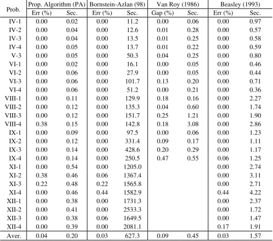
Table 1 presents the computational results for Kuehn & Hamburger (1963) test problems.
The data was obtained from Beasley’s (1990) OR-Library. Problems IV-VI are 16 50× ,
problems VIII and IX are 25 50× and problems XI and XII are 50 50× . The first number relates to potential plant locations and the second to the number of demand centers. Van Roy (1986) uses a different numbering.
The second column of Table 1 shows that the relative difference between the solution value obtained by PA and the optimal value was always under 0.4%. For 22 out of 25 problems, i.e. 88%, the optimal solution was found. Times were always under 0.55 seconds.
Table 1 – Computational results based on Kuehn and Hamburger data.
Prop. Algorithm (PA) Bornstein-Azlan (98) Van Roy (1986) Beasley (1993) Prob. Err (%) Sec. Err (%) Sec. Gap (%) Sec. Err (%) Sec.
IV-1 0.00 0.02 0.00 11.2 0.00 0.06 0.00 0.97 IV-2 0.00 0.04 0.00 12.6 0.01 0.28 0.00 0.57 IV-3 0.00 0.04 0.00 13.5 0.01 0.25 0.00 0.58 IV-4 0.00 0.05 0.00 13.7 0.01 0.22 0.00 0.59 V-3 0.00 0.05 0.00 50.3 0.04 0.25 0.00 0.80 VI-1 0.00 0.02 0.00 16.1 0.00 0.05 0.00 0.46 VI-2 0.00 0.06 0.00 27.9 0.00 0.05 0.00 0.44 VI-3 0.00 0.06 0.00 101.7 0.13 0.20 0.00 0.71 VI-4 0.00 0.06 0.00 51.2 0.00 0.21 0.00 0.36 VIII-1 0.00 0.11 0.00 129.9 0.18 0.16 0.00 2.27 VIII-2 0.00 0.12 0.00 135.3 0.04 0.60 0.00 1.74 VIII-3 0.00 0.12 0.00 151.7 0.25 1.21 0.00 1.90 VIII-4 0.38 0.15 0.00 142.8 0.18 3.08 0.00 2.86 IX-1 0.00 0.09 0.00 97.5 0.00 0.06 0.00 1.23 IX-2 0.00 0.12 0.00 331.4 0.09 0.17 0.00 1.11 IX-3 0.00 0.14 0.00 428.6 0.20 0.29 0.00 1.17 IX-4 0.00 0.14 0.00 250.5 0.47 0.55 0.06 1.25
XI-1 0.00 0.54 0.00 1205.0 0.00 2.74
XI-2 0.38 0.46 0.06 1367.4 0.00 3.11
XI-3 0.22 0.48 0.22 1565.8 0.00 2.71
XI-4 0.00 0.46 0.44 1582.9 0.44 4.22
XII-1 0.00 0.38 0.00 1731.3 0.00 2.37
XII-2 0.00 0.41 0.00 2533.3 0.00 1.72
XII-3 0.00 0.38 0.06 1649.5 0.00 1.47
XII-4 0.00 0.39 0.00 2081.1 0.17 1.91
Although numbers from Table 1 give an idea about the efficiency of each algorithm, comparisons have to be made very carefully. To measure the quality of the solution, PA, Bornstein & Azlan (1998) and Beasley (1993) use the relative difference (ERR%) between the solution value obtained by the algorithm and the optimal value. However, for Bornstein-Azlan, ERR% is calculated taking the best solution of a 5-run of each problem. Considering an average value instead of the best value for the 5-run, shifts the average ERR% for the 25 problems from 0.03% to 0.13% ! On the other hand, Van Roy (1986) evaluates his solutions using the relative duality gap (GAP%) which only provides an upper bound for ERR%. The fact that Van Roy does not give the value of the generated solutions unfortunately makes it impossible to calculate ERR% for his results at Table 1.
With respect to times only the first two algorithms can effectively be compared, since similar machines were used. The SAE-best algorithm presented by Bornstein & Azlan (1998) expends much more time than PA. Also Beasley (1993) and Van Roy (1986) are computationally more expensive than PA. Although times of the first two algorithms are almost equivalent to times spent by PA, one has to consider that they were run on more powerful machines. One should also take into account that both Beasley (1993) and Van Roy (1986) provide upper and lower bounds for the optimal solution.
Summing up, a good trade-off seems to exist for PA between the quality of the solution and the computational time. This is what should be expected from a heuristic.
To test the performance of PA for larger instances, we considered 100 1000× randomly
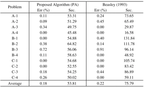
generated problems available at Beasley’s (1990) OR-Library. Table 2 compares PA only with Beasley (1993) because for the other algorithms data was not available for problems of this dimension. The relative error of PA was always less than 0.75%, but for only 4 out of 12 problems the optimal solution was obtained. Times were less than one minute. Again, PA obtains solutions with quality similar to those obtained by Beasley (1993). Times, however, are much smaller.
Table 2 – Computational results based on Beasley data.
Proposed Algorithm (PA) Beasley (1993) Problem
Err (%) Sec. Err (%) Sec.
A-1 0.11 53.31 0.24 73.65 A-2 0.09 51.29 0.45 65.49 A-3 0.34 49.75 0.00 29.87 A-4 0.00 45.48 0.00 16.58
B-1 0.00 54.88 0.40 131.84
B-2 0.38 64.82 0.14 111.78
B-3 0.72 56.06 0.91 96.14 B-4 0.11 58.63 0.00 48.92
C-1 0.00 54.68 0.00 105.74
C-2 0.00 52.55 0.00 83.42 C-3 0.18 54.25 0.44 86.89 C-4 0.26 50.02 0.00 59.11
5. Conclusions
A central dilemma of the CPLP is the conflict between the minimization of fixed and variable costs each driving the solution in a different direction. The minimization of variable/transportation costs in the extreme case forces the solution towards putting a plant near each demand center i.e. represents a tendency towards decentralization. On the other hand, due to economies of scale, fixed costs are generally minimized by placing a central unit which supplies all demand centers. Of course, the joint minimization of fixed and variable costs means that there needs to be a compromise between the centralization and decentralization tendencies.
The algorithm presented in this paper moves around this dilemma, detecting dominances among the two types of costs and locating plants according to these dominances. The computational results show that it is able to tackle large scale problems finding almost always near optimal solutions at very low cost.
However not everything is as positive as it may seem. The Achilles’ heel is the shortsightedness of the algorithm, i.e. the tendency to act only locally, determining whether each plant should be opened or not sequentially. One should not forget that the dilemma mentioned above is a global question where all the complex interrelations between the various plants and demand centers play an important role. To counterbalance this tendency the algorithm has at phase 2 an interchange heuristic which tries to detect relations between plants.
Detecting dominances locally may lead to distortions with respect to determining a global optimal solution. These distortions may heavily rely on data. This is the reason for introducing parameters which may correct these distortions. In the sense of greater transparency only one parameter was introduced in the algorithm. Greater values of
ε
make it easier to close plants at phase 1. Closed plants are not further examined at phase 2. On the other hand smaller values of ε result in putting plants in K0 instead of K0. Plants in K0will be examined again at phase 2 and are object of the interchange heuristic. As a general principle one should have in mind that decreasing ε generally leads to better solutions at a higher computational cost. For the set of tested problems, using
ε
equal to 0.05 seems to lead to the best value solution, i.e. leads to the best possible solution within a reasonable computational cost. Decreasingε
further down may only lead to a very slight improvement of the solution at a much higher computational cost.Acknowledgments
The authors are partially supported by CNPq (grants nr. 523158/94-7 and 300251/00-9) and FUJB (grant nr. 5561-1).
References
(1) Ahrens, J.H. & Finke, G. (1980). Primal Transportation and Transshipment Algorithms. Zeitschrift fur Operations Research, 24, 1-32.
(2) Akinc, U. & Khumawala, B.M. (1977). An Efficient Branch and Bound Algorithm for the Capacitated Warehouse Location Problem. Management Sci., 23, 585-594.
(3) Azlan, H.A.B. (1995). Aplicação do Algoritmo Simulated Annealing ao Problema de Localização Capacitado, Usando Testes de Redução (The Use of Simulated Annealing for the Capacitated Plant Location Problem Using Reduction Tests). D.Sc. Thesis, COPPE/UFRJ, Rio de Janeiro.
(4) Barcelo, J.; Fernandez, E. & Jörnsten, K.O. (1991). Computational Results from a New Lagrangean Relaxation Algorithm for the Capacitated Plant Location Problem. European J. Operational Research, 53, 38-45.
(5) Beasley, J.E. (1988). An Algorithm for Solving Large Capacitated Warehouse Location Problems. European J. Operational Research, 33, 314-325.
(6) Beasley, J.E. (1990). OR-Library: distributing test problems by electronic mail. J. Operational Research Soc., 41, 1069-1072.
(7) Beasley, J.E. (1993). Lagrangean Heuristics for Location Problems. European
J. Operational Research, 65, 383-399.
(8) Bornstein, C.T. & Azlan, H.B. (1998). The Use of Reduction Tests and Simulated Annealing for the Capacitated Plant Location Problem. LocationSci., 6, 67-81.
(9) Christofides, N. & Beasley, J.E. (1983). Extensions to a Lagrangean Relaxation
Approach for the Capacitated Warehouse Location Problem. European J. Operational
Research, 12, 19-28.
(10) Cornuejols, G.; Sridharan, R. & Thizy, J.M. (1991). A Comparison of Heuristics and
Relaxations for the Capacitated Plant Location Problem. European J. Operational
Research, 50, 280-297.
(11) Holmberg, K. & Ling, J. (1995). A Lagrangean Heuristic for the Facility Location Problem with Staircase Costs. Technical Report LiTH-MAT-R-1995-24, Linköping University, Sweden.
(12) Jacobsen, S.K. (1983). Heuristics for the Capacitated Plant Location Problem. European J. Operational Research, 12, 153-261.
(13) Kuehn, A.A. & Hamburger, M.J. (1963). A Heuristic Program for Locating Warehouses. Management Sci., 9, 643-666.
(15) Nemhauser, G.L. & Wolsey, L.A. (1988). Integer and Combinatorial Optimization. J. Wiley & Sons.
(16) Thizy, J.M. (1994). A Facility Location Problem with Aggregate Capacity. INFOR, 32, 1-18.
(17) Van Roy, T.J. (1986). A Cross Decomposition Algorithm for Capacitated Facility Location. Operations Research, 34, 145-163.
(18) Wolsey, L.A. (1983). Fundamental Properties of Certain Discrete Location Problems.