THE PHILLIPS CURVE AND INFORMATION RIGIDITY
IN BRAZIL
Sidney M. Caetano* Guilherme V. Moura†
Abstract
This work aims at testing the null hypothesis of no sticky information against the alternative of sticky information using Brazilian data. The rejection of the null hypothesis allows us to derive the expected time be-tween information updates. The median of market participants’ predic-tions collected by Gerin/Bacen is used as a proxy to firms’ expectation contained in the sticky information version of the Phillips curve. Our esti-mates imply that inflation expectations in Brazil are updated about once each five quarters, which in part can be attributed to reduced uncertainty about Brazilian inflation in the period of analysis.
Keywords: Phillips Curve, Sticky Information, Inflation Expectations.
Abstract
O objetivo deste trabalho é testar a hipótese de ausência de rigidez de informação no Brasil. A metodologia permite também derivar a frequên-cia de reajuste informacional via Curva de Phillips sob Rigidez de Infor-mação. Para tanto, a mediana das projeções de mercado divulgadas pela Gerin/Bacen são utilizadas comoproxypara as expectativas contidas na curva de Phillips. As estimativas obtidas são consistentes com o modelo e implicam em atualização de informação a cada cinco trimestres. Portanto, o período de atualização de informações estimado para o Brasil é próximo de alguns estimados para países europeus e norte americanos, o que em parte pode ser atribuído à redução nas incertezas inflacionárias brasileiras no período de análise.
Keywords:Curva de Phillips, Rigidez de Informação, Expectativas de In-flação.
JEL classification:E31,D84
*Departamento de Economia, Universidade Federal de Viçosa. Email: [email protected].
†Programa de Pós-Graduação em Economia, UFSC. Email: [email protected]
1
Introduction
The stylized facts about inflation dynamics indicate that: i) monetary pol-icy actions require some lags to have their full impact on inflation; ii) there is a high serial correlation in inflation; iii) disinflation policies have contrac-tionary effects; and iv) monetary policy actions have their maximum effects on
cyclical output before they have their maximum effect on inflation (see (Khan
& Zhu 2006) for US evidence, and (Döpke et al. 2008) for european stylized facts).
BACEN (2007) shows that Brazilian output gap initially reacts with a lag of one quarter after changes in the interest rate, while inflation response to output gap changes occurs one or two quarters afterwards. Thus, monetary policy effects occurs with lags in Brazil as well. The high persitency in
Brazil-ian inflation is studied in Campêlo & Cribari-Neto (2003), and Tombini & Alves (2006) show that disinflationary policies have contractionary effects in
Brazil.
The stylized facts in Brazil show that the Brazilian output gap initially reacts with a lag of one quarter after changes in the interest rate, while the inflation response to the output gap occurs one or two quarters afterwards, (BACEN 2007, p.120-21). Therefore, it can be observed that the first inflation reaction to variations in the output gap only occurs two or three quarters af-ter the change in the inaf-terest rate. The maximum effect upon inflation occurs
even later than that. One of the important characteristics of the dynamics of inflation in Brazil is its degree of persistence or serial correlation. In the eight-ies until the mid-nineteight-ies, this was a serious problem where the economy had a high degree of inertia. Later, after the Real Plan, the inertia showed a strong decline. Campêlo & Cribari-Neto (2003) show that the inertial component in the Brazilian inflationary dynamics is second order. Tombini & Alves (2006) show that there was an increase in the cost of disinflation.
The search for an explanation of these facts has led to great discussion and the development of explanatory models, such as the New Keynesian models of price rigidity. This class of models is based on the seminal work of Taylor (1980) and Calvo (1983), and has offered a Phillips curve where current
in-flation is determined by the current output gap and current expectations of future inflation.
Based on the concept of "sticky information", Mankiw & Reis (2002) pro-posed a new model to solve the puzzle of the inertia in inflation and to explain the dynamic effects of aggregate demand on output and on the price level.
According to their theory, companies do not immediately update their old information. The main aspect of the model is that information about macroe-conomic conditions diffuses slowly through the population. They assume
pre-determined prices, which result from the costs of acquiring information and processing information, or costs of reoptimization (sticky information). Com-panies may decide not to continuously update their prices, choosing a trajec-tory for them, which would be followed until new information collection and processing are performed. Such behavior is based on the rationale that there are costs associated to obtaining and processing information. In the model, the specification of the inflation dynamics is given by what Mankiw & Reis (2002) called the "sticky-information Phillips curve” (SIPC).
the effects of monetary policy: disinflations are always contractionary;
mone-tary policy shocks have their maximum impact on inflation with a substantial delay; and the change in inflation is positively correlated with the level of economic activity. These characteristics, as mentioned above, are common to different economies, including Brazil.
Faced with the evolution of the research on Phillips curve, and with the discussion about information rigidity as an alternative way to sustain a slow adjustment of prices, it is important to investigate the empirical performance of the Phillips curve under sticky information using Brazilian data. Despite the growing international literature on this topic, not many studies about the existence or not of some degree of information rigidity in Brazil are available, and this work tries to fill this gap.
The implications of the sticky-information model are closer to those of Fischer’s contracting model, (see Fischer 1977). A key feature of the SIPC is that current inflation depends not only on current output gap, but also on past expectations of inflation and the growth rate of the current output gap. However, there is no clear hint on how to proxy these past expectations of inflation. Khan & Zhu (2006) use a method based on out of sample predictions obtained via an estimated VAR to proxy firms’ expectations. Gorodnichenko (2006), on the other hand, uses the Michigan survey of consumer expectations, and Döpke et al. (2008) uses the median of market participants’ predictions to proxy firms’ expectations contained in the aforementioned version of the Phillips curve.
This feature complicates the estimation of the empirical SIPC. At this point, we use nonlinear least squares to estimate the degree of information rigidity in the Brazilian economy, which will be determined by the parameterλ. We use the empirical approach of Döpke et al. (2008) to test of the null hypothesis of no information rigidity (λ= 1) against the alternative of sticky information (λ,1), which is a test to verify if the model from Mankiw & Reis (2002) is valid in Brazil. Guillèn (2008) also estimates the SIPC model for Brazilian data. However, he uses the method of Khan & Zhu (2006) to model firms’ inflation expectation.
Guillèn (2008) presents essays about the expectations of inflation in Brazil, focusing on information rigidity, and information readjustment. The author is concerned about the dispersion of the expectations, its median and the ap-plication of the Gorodnichenko (2006) proposal to evaluate the information rigidity theory. Some results corroborate the literature, while others were not predicted by the theory. Guillèn (2008) uses a method different from ours
to proxy firm’s expectations, which is based on out of sample predictions ob-tained via an estimated VAR. His results suggest that a company takes about six months to readjust its information set.
Our estimates imply that inflation expectations in Brazil are updated about once each five quarters, which in part can be attributed to reduced uncertainty about Brazilian inflation in the period of analysis. This value is compatible with the average duration among the updates of information for American firms estimated by Khan & Zhu (2006). Brazilian companies would be ex-pected to update their information about the level of prices more often, due to Brazilian hyperinflation experienced in the past. However, since the pe-riod analyzed is characterized by economic and price stability, the costs for information update may be higher than the costs of inflation in this period.
present the Phillips curve under information rigidity. Section 2 discusses the methodology and the data set used, and section 3 deals with the results and discusses them. Some conclusions are drawn in section 4.
2
The Role of Inflation Expectation
The way agents determine, transmit, and update their expectations has re-ceived great attention from scholars and policy makers in recent decades, since they are important for understanding the transmission mechanism of monetary policy.
Friedman (1968) and Phelps (1969) used adaptive expectations to explain the phenomenon of stagflation. However, the hypothesis of adaptive expec-tations was criticized, since the expected inflation should not take into con-sideration only previous inflation. Lucas (1973), based on the work of Muth (1961), increased the information set used when considering expectations in a Phillips curve. Thereafter, economic models started to take into consideration this broader idea of expected inflation, using not only past inflation to form expectations but also all the information available to the economic agents. In spite of criticism, such hypothesis has been considered more realistic and has been employed in several economic models thereafter.
In the 80s, based on the work of Taylor (1980), Tybout & R. (1995) pro-posed a Phillips curve model, where price rigidity plays an important role, and where current inflation depends on the output and on the expectations about future inflation. This model became known as theNew Keynesian Phillips Curve. However, a series of puzzles were detected in this model, namely: cred-ible disinflation would generate expansion instead of recession; the persis-tence of inflation would not be explained; and, finally, the gradual response to real shocks in such model would not be justifiable.
Mankiw & Reis (2002) have recently constructed a model of New-Keynesian Phillips Curve in which the rigidity is of information instead of prices, but that would still support a slow price adjustment. Following the concept of expectations under rigid information, they argue that agents may use all avail-able information to form their expectations, but, due to costs in obtaining and processing this information, agents and firms do not update their expectations every time period. In this sense, the hypothesis of sticky information does not exclude the hypothesis of rational expectations, because even having constant access to information, agents prefer to maintain the information set lagged to avoid costs in processing the new information1.
According to Döpke et al. (2008), information rigidity would be observed for countries such as Germany, France, Italy and the United Kingdom. For Italy, the readjustment of the expectations would take place every six months, while for the other countries, the gap would be of one year.
Next, we briefly present the standard New Keynesian Phillips Curve based on sticky prices, and derive the model of sticky information from Mankiw & Reis (2002).
1Mankiw et al. (2004) investigate if inflation expectations in the United States are either based
2.1 The New Keynesian Phillips Curve
A model widely used to derive the Phillips Curve is the one proposed by Calvo (1983), which assumes that the readjustment of prices by each company is not synchronized with the readjustment of the others. Each company readjusts its price randomly when it receives a signal. The probability of receiving the signal in this period is equal toλand the average time until a price adjustment is equal toλ1. Therefore, the probability that the readjustment of prices occurs injperiods is given by:
P(X=j) =λ(1−λ)j−1, j= 1,2, . . . .
This probability does not depend on the past history of updates. Thus, the expected time between updates of information is λ1, since the average time until a price adjustment is equal to the expectation of random variables of the geometric distribution:
E[X] = ∞ X
j=1
jP(X=j) = ∞ X
j=1
jλ(1−λ)j−1=1
λ (1)
For example, when λ = 0.5 in a model for quarterly data, the average time of readjustment will be two quarters. The parameter λcan also be seen as the fraction of firms that use the updated information in their decisions about prices. The remaining fraction of firms, 1−λ, continues to use old or outdated information.
The New Keynesian Phillips Curve based on the model of Calvo (1983) has three important relations. The first one gives the desired price the firm wants to charge:
p∗
t=pt+αyt, (2)
where the current desired pricep∗
t is a function of current outputytand the current price level pt2. In fact, y should be interpreted as an output gap, since the potential product is normalized to zero. Equation (2) shows that the desired relative price increases in the periods of growth and decreases in recessions, and thatα refers to the sensitivity of the optimal price to the current output gap.
The second relation shows that when a firm has the opportunity to change the price, it adjusts its price by making a weighted average of the current desired price and all the prices desired in the future:
xt=λ ∞ X
j=0
(1−λ)jEt[pt+j∗ ], (3)
where the future desired prices receive lower weights as the horizon increases. The third equation reveals how the price level is determined:
pt=λ ∞ X
j=0
(1−λ)jxt−j, (4)
where the level of prices is a weighted average of prices prevailing in the model economy.
The solution to these three last equations leads to the New Keynesian Phillips Curve:
πt= αλ 2
1−λ !
yt+Et[πt+1], (5)
which states that the inflation rateπt =pt−pt−1 today is a function of the output gap, and of next period’s expected inflation.
A small value ofαmeans that a firm’s desired relative price is not very sen-sitive to macroeconomic conditions. Thus, ifα is small, then each firm gives more weight to what other firms are charging than to the level of aggregate demand.
The New Keynesian Phillips Curve can be written in a more compact form as follows:
πt=βyt+Et[πt+1], (6)
whereβ=αλ1 2 −λ
.
2.2 The Phillips Curve under Information Rigidity
Mankiw & Reis (2002) presented an alternative model for the dynamics of prices, where in each period, a fraction of firms updates their optimal price trajectory given the currently available information. Other firms remain with their optimal trajectories based on lagged information.
It is a closed economy model, where firms are expected to work in a mo-nopolistic competition environment. The firm chooses the optimal price in each period, but the information used to calculate this optimal price is not necessarily up-to-date information, implying that information is sticky. In other words, in contrast to the model of sticky prices, the prices are always changing, but some prices are based on old and outdated information.
Firms form their expectations rationally, but because of the costs associ-ated to the update of old information or new information processing, the ex-pectations do not change very often.
Similarly to the previous model of the New Keynesian Phillips Curve, the optimal price of the firm is given by (2). However, the firm that updated its plansjperiods ago set its price according to:
xtj=Et−j[pt∗]. (7)
pt=λ ∞ X
j=0
(1−λ)jxjt. (8)
Using equations (2), (7), and (8), a new equation for the price level is de-rived:
pt = λ ∞ X
j=0
(1−λ)jEt−j[pt+αyt], (9)
= λ(pt+αyt) +λ ∞ X
j=0
(1−λ)j+1Et−j−1[pt+αyt]. (10)
The price level for the immediately preceding period is
pt−1=λ ∞ X
j=0
(1−λ)jEt−j−1[pt−1+αyt−1]. (11)
Subtracting (11) from (10), we obtain the equation for the inflation rate
πt=λ(pt+αyt) +λ ∞ X
j=0
(1−λ)jEt−j−1[πt+α∆yt] (12)
−λ2 ∞ X
j=0
Et−j−1[pt+αyt].
Now, equation (10) can be used to show that:
pt−
αλ
1−λ
yt = λ ∞ X
j=0
(1−λ)jEt−j−1[pt+αyt]. (13)
Using (13) to replace the last term in (12), we obtain the Phillips Curve under sticky information
πt=
αλ
1−λ
yt+λ ∞ X
j=0
(1−λ)jEt−j−1[πt+α∆yt], (14)
where∆yt=yt−yt
−1is the growth of the output gap. Therefore, the inflation rate depends on the output gap, inflation expectations and expectations of output gap growth.
It is important to note that prices do not need to be sticky. In the sticky price model, current expectations of the future economic conditions play a relevant role in determining the inflation rate. In information rigidity, on the other hand, past expectations of the current conditions are highlighted, generating a different price and output dynamics as a response to changes in
Furthermore, in an empirical study on the sticky information Phillips curve, the parametersα andλshould be estimated, thus determining the sensitiv-ity of the optimal price to the current output gap, and the frequency of in-formation readjustment, respectively, i.e., the estimated structural parame-ter λrefers to the degree of information rigidity, and a higher value means that many firms use the updated information when determining their prices, which leads to a smaller degree of information rigidity. Therefore, inflation becomes more sensitive to the current output gap and less sensitive to the past expectations of the current inflation and the growth rate of the current output gap. The parameterαcan also be interpreted as the real degree of rigidity, as discussed by Ball & Romer (2003).
3
Methodology and Data
From the empirical point of view, the specification of the sticky information Phillips Curve given in (14) involves old expectations of present events, such as the inflation rate and the output gap. The first step for the estimation of this model is to determine how these expectations included in the sticky information Phillips Curve are calculated.
Khan & Zhu (2006) carry out an analysis for the United States, Canada and the United Kingdom, using out of sample forecasts based on a VAR model as proxy for the expectations contained in (14). Guillèn (2008) adopts the same strategy for Brazilian data, while Döpke et al. (2008) analyze European data using expectations for the inflation and for the output gap based on the median of the expectations of several institutions collected in a survey.
Here, an approach similar to that of Döpke et al. (2008) will be used, where the median of the market projections published by the Gerin/Bacen 3 will serve as proxy for the inflation expectations contained in (14). This approach seems to be more reasonable, once the hypothesis that the companies con-struct their expectations based on market projections, widely available in the Gerin/Bacen website, seems more likely to us than the hypothesis that compa-nies construct a VAR model to serve as the basis for their expectations related to several future events. Moreover, since Guillèn (2008) already analyses this issue using the approach of Khan & Zhu (2006), it seems natural to evaluate the results of a different approach. According to Central Bank of Brazil (2004,
p. 116), out of 104 informants, 84 were financial institutions (52 banks, 23 resource administrators, and 9 brokerage firms and distributors), 14 consul-tancy companies and 6 non-financial companies and class entities. The Cen-tral Bank of Brazil argues that, in practice, companies and entities, regardless of their sector, present smaller capacity to respond to macroeconomic changes than the participants of the financial sector and consultancy companies, due to the very nature of their professional activity, mainly in the presence of data of high frequency and/or in an environment of volatilities.
Another aspect to be pointed out in equation (14) is the infinite sum of past expectations. In any empirical study on the sticky information Phillips curve, this sum has to be truncated at some pointjmax. Given that the Gerin/Bacen collects projections four or five steps ahead, jmax will be fixed at 3. In this point, the approach based on projections of a VAR model is advantageous,
3The reference dates follow the last working day, previously to the date when the IPCA-15 is
since jmax can be fixed at a higher value, taking into consideration expecta-tions formed in a more distant past, although it still has to be truncated at some point. In order to analyse the effect of the truncation lag jmax used in
the summation of the empirical version of (14), we present results based on bothjmax= 2 andjmax= 3 in Table 1 and 2.
Data about expectations for the output gap and for the inflation are con-structed as in Döpke et al. (2008), where the growth expectations of the GDP together with the data of the effective GDP are combined to form a series of
ex-pected GDP. This series is then filtered in a way to decompose the logarithm of the original series into potential output (trend) and cyclical movements, characterizing the output gap. To guarantee the robustness of the results with respect to the filter used, both the Christiano & Fitzgerald (2003) bandpass fil-ter and the HP filfil-ter developed by Hodrick & Prescott (1997) were used. Time series of the GDP for the first quarter of 2001 until the first quarter of 2009 were obtained at the IBGE website in table 1620 of the Sidra.
The IPCA is used as a price index, and the medians of the projections for the growth rate of the IPCA4 are used to construct the expected IPCA time series for one, two, three and four steps ahead, exactly as it was done for GDP. The data for the IPCA general index were collected at the Ipeadata website for the same period, while the medians of the projections of the GDP and IPCA growth were obtained at the website of Banco Central do Brasil for the fourth quarter of 2001 until the first quarter of 2009.
Due to the nonlinear characteristic of equation (14), the method of nonlin-ear least squares (see Davidson & MacKinnon 1993) is used to estimate the sticky information Phillips curve model. Therefore, the regression equation estimated was:
πt=xt(β) +ut, ut∼i.i.d(0, σ2) (15)
wherext(β) is a nonlinear function ofβ, which determines the conditional mean ofπtwith respect to the independent variables used, and is given by
xt(β) =
αλ
1−λ
yt+λ 3 X
j=0
(1−λ)jEt−j−1[πt+α∆yt]. (16)
The parametersβ= (α, λ) are estimated as the ones that minimize the sum of the squared residuals. For the model describe by (15) and (16), the function to be minimized is
SSR(β) = T X
t=1
(πt−xt(β))2= (π−x(β))′(π−x(β)), (17)
4Studies for Brazil show that market inflation forecasts do not conform to the strict
rational-ity hypothesis. Carvalho & Bugarin (2006) found that, although market forecasts did not show systematic biases, they were not efficient in the use of the information available with respect to
where the last equality is simply the matrix representation ofSSR(β).
The first order conditions for the minimum are achieved by differentiating
(17) with respect to the vector of parametersβ. The parameter estimatesbβare the ones that satisfy
−2X(βb)′π+ 2X(bβ)′x(bβ) = 0, (18)
whereX(βb) is a (T×2) matrix containing the partial derivatives ofxt(β) with respect to βand evaluated at the bβvalues. Estimates of the standard errors associated with theβbestimates are given by
s(bβ) = r
s2X(bβ)′X(bβ)−1, (19)
wheres2 is an estimate of the variance of the error term in equation (15), which is given by (T−2)−1SSR(βb). A Newton-Raphson’s type algorithm was
used to find the fixed point of the system given by the first order conditions in (18) with a convergence criterion of 1.0E−08.
4
Results and Discussion
4.1 A Sensitivity Analysis
Khan & Zhu (2006) argue that sinceαdepends on the structural parameters of the model economy, it is not possible to precisely estimate it together with
λ. Therefore, these authors fixedαto either 0.10 or 0.15. These values are con-sidered the most likely also by Mankiw & Reis (2002) and Woodford (2003), and they imply strategic complementarities in the decisions about price ad-justment of the firms. The alternative α = 0.2 is included by Döpke et al. (2008) for European data, and by Guillèn (2008) for Brazilian data.
We tried to jointly estimate the parametersλandα, but the estimates of
αandλwere very imprecise, exactly as described by Khan & Zhu (2006), and Döpke et al. (2008). Therefore, we adopted the same strategy, used by them, and fixedαto either 0.10, 0.15 or 0.20.
The results of the estimates ofλare presented in Table 1 and 2. The hy-pothesis to be tested is H0: λ= 1, which would imply the non-existence of information rigidity, against the alternative hypothesis H1: λ <1, implying some degree of information rigidity.
The estimates ofλare statistically different from 1, supporting the sticky
information Phillips curve model presented in the section 2.2. The null hy-pothesis of non-existence of information rigidity can be rejected with 99% of confidence for all the different values ofα, and for both filters used for the
calculation of the output gap. In contrast to Khan & Zhu (2006) and Döpke et al. (2008), the estimates ofλfor the Brazilian case are not very sensitive to the value ofα. However, the estimates ofλare more sensitive to the trunca-tion lagjmax used in the summation of the empirical version of (14). Table 1 presents results based onjmax= 2, while Table 2 contains results based on
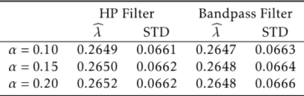
Table 1: Estimates of the Sticky Information Phillips Curve forjmax= 2
HP Filter Bandpass Filter b
λ STD bλ STD
α= 0.10 0.2649 0.0661 0.2647 0.0663
α= 0.15 0.2650 0.0662 0.2648 0.0664
α= 0.20 0.2652 0.0662 0.2648 0.0666
Note: Estimates are based on observations from the third quarter of 2002 to the first quarter of 2009. Data on inflation expectation is based on end of the quarter projections made one working day before the release of IPCA-15.
Table 2: Estimates of the Sticky Information Phillips Curve forjmax= 3
HP Filter Bandpass Filter b
λ STD bλ STD
α= 0.10 0.2036 0.0542 0.2035 0.0543
α= 0.15 0.2037 0.0542 0.2035 0.0543
α= 0.20 0.2038 0.0542 0.2035 0.0544
Note: Estimates are based on observations from the fourth quarter of 2002 to the first quarter of 2009. Data on inflation expectation is based on end of the quarter projections made one working day before the release of IPCA-15.
based onjmax = 2 and onjmax = 3 are somewhat large, they are not statisti-cally significant given the standard errors presented and the difference in
es-timates could be only due to estimation error associated with a finite sample. As the original summation in (14) goes to infinity, we favor the results based onjmax= 3, although both summation are still very poor approximations to an infinite summation. The fact that the λ estimates decrease from around 0.265 to 0.203 might be seen as an evidence that the infinite summation has not converged yet. However, it will only be possible to achieve a better ap-proximation to (14) using actual market predictions when more data about price and output expectations in Brazil are available.
Results in Table 2, imply an average estimate forλ= 0.2036. Using this value to calculate the average duration among the updates of information, we obtain 0.20361 = 4.9116. This means that, on average, firms update their information about the evolution of prices every five quarters. This value is compatible with the average duration among the updates of information for American firms estimated by Khan & Zhu (2006).
4.2 Inflation and Output Dynamics
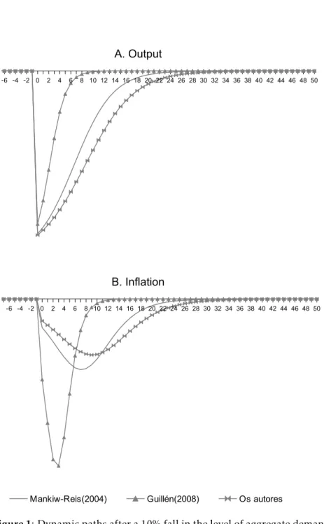
Following the experiments of Mankiw & Reis (2002), we now consider three hypothetical policy experiments, where we posit a path for aggregate demand
mt. We then derived the path for output and inflation generated by the sticky-information model estimated in this paper and compared it with the paths generated by the sticky-information models of Mankiw-Reis and Guillèn (2008). The details of the solution are presented in the appendix of Mankiw & Reis (2002).
In order to do this exercise, we need to introduce in the model an equation for aggregate demand,mt=pt+yt. This equation can be viewed as a quantity-theory approach to aggregate demand. Alternatively,mcan be viewed more broadly as incorporating the many other variables that shift aggregate de-mand. We considermas exogenous.
We simulate three scenarios based onα= 0.1, where the first one is based on our estimates andλ= 0.2036; the second one is based on Mankiw & Reis (2002) and setsλ= 0.25; and the third one hasλ= 0.5 as estimated by Guil-lèn (2008). Based on Mankiw-Reis’ estimates, firms make, on average, adjust-ments once a year. Based on Guillén, about once each two quarters, and based on our estimates, inflation expectations in Brazil are updated about once each five quarters.
A drop in the level of aggregate demand
The first experiment we consider is a sudden and permanent drop in the level of aggregate demand. The demand variablemt is constant and then, at time zero, it unexpectedly falls by 10 percent and remains at this new level.
The top graph in Figure 1 shows the path of the output predicted by each of the three calibrations. In all three, the fall in demand causes reces-sion, which gradually dissipates over time, faster in the calibration of Guillèn (2008). The impact of the fall in demand on output is close to zero at ten quar-ters and twenty-five quarquar-ters, following our calibration and that of Guillén, re-spectively. In the calibration of Mankiw-Reis, the impact of the fall in demand on output is close to zero at twenty quarters. In the bottom of Figure 1, we examine the response of inflation. In Guillén’s calibration, the greatest impact of the fall in demand on inflation occurs almost immediately. The other two calibrations show a more gradual response. In the sticky-information model based on Mankiw-Reis’ results, the maximum impact of the fall in demand on inflation occurs at seven quarters; based on our estimates, the maximum impact is reached in the nineth quarter; and based on Guillén’s in the third quarter.
A sudden disinflation
Here we consider a sudden and permanent shift in the rate of demand growth. The demand variablemtis assumed to grow at 10 percent per year (2.5 percent per period) untilt= 0. In periodt= 0, the central bank setsmt at the same level as it was in the previous period and, at the same time, announces that
mt will remain constant thereafter. Figure 2 shows the path of output and inflation predicted by the three calibration.
! " # ! $
based on Guillén’s estimate predicts faster reduction in inflation. For Mankiw & Reis (2002), even after the disinflationary policy is in force, most price set-ters are still marking up prices based on old decisions and outdated informa-tion. With a constant money supply and rising prices, the economy experi-ences recession, which reaches its trough six quarters after the policy change based on Mankiw-Reis’ estimates; two quarters, based on Guillén; and eight quarters, in our case. Then, output gradually recovers and is almost back to normal after twenty quarters in Mankiw-Reis’s case; after ten quarters in Guillén’s; and thirty quarters in our case.
! " # ! $
An anticipated disinflation
Now suppose that the disinflation in our previous experiment is announced and credible two years (eight periods) in advance. Let us consider how this anticipated disinflation affects the path of output and inflation.
Figure 3 shows output and inflation according to the three models. The sticky-information model does not produce booms in response to anticipated disinflations. Based on Mankiw-Reis’ estimate and based on our estimates, there is no change in output or inflation until the disinflationary policy of slower money growth begins. After that, based on our model, the disinflation causes a higher recession. Based on Guillén’s estimates, the announcement has no effect on the inflation or output. Because of the announcement, many
price setters have already adjusted their plans in response to the disinflation-ary policy.
5
Conclusion
The present study focused on the test of the null hypothesis of no information rigidity (λ= 1) against the alternative of sticky information (λ,1), which is a test of whether the model from Mankiw & Reis (2002) is valid in Brazil. The rejection of the hypothesis allows us to derive the expected time between infor-mation updates. The approach used was similar to that of Döpke et al. (2008), where the median of the market projections released by the Gerin/Bacen were used as proxies for the expectations contained in the Phillips Curve.
The estimated structural parameterλ represents the degree of informa-tion rigidity, and a higher value ofλmeans that many firms use the updated information when determining their prices, which leads to a smaller degree of information rigidity. Therefore, inflation becomes more sensitive to the current output gap and less sensitive to the past expectations of the current inflation and the growth rate of the current output gap. The parameter α
captures the sensitivity of the optimal price to the current output gap. It can also be interpreted as the real degree of rigidity, as discussed by Ball & Romer (2003).
The results of the present work revealed that the null hypothesis of non-existence of information rigidity can be rejected at the 99% confidence level, which implies that Brazilian firms do not adjust their information related to the price level instantaneously. In addition, the estimates suggest that compa-nies take about five quarters to update their information about future prices. Therefore, the period of information readjustment in Brazil can be compared to that of European and American countries, maybe partly due to the reduced inflation uncertainties in Brazil during the period of the analysis. However, more precise estimates of the average duration between information updates by companies will only be possible as more data about price and output expec-tation in Brazil become available. This would not only allow the corroboration of the results presented here, but also a deeper investigation about the main determinants of the time needed for Brazilian firms to adjust their informa-tion.
Still, according Mankiw & Reis (2002), the sticky information model dis-plays three related properties that are more consistent with accepted views about the effects of monetary policy: disinflations are always contractionary,
sub-! " # ! $
stantial delay, and changes in inflation are positively correlated with the level of economic activity.
Bibliography
BACEN (2007), Banco central do Brasil. análise do mercado de câmbio. 1998-2007, Technical report, Banco Central do Brasil.
Ball, L. & Romer, D. (2003), ‘Inflation and the informativeness of prices.’, Journal of Money, Credit and Banking.35(2), 177–196.
Calvo, G. (1983), ‘Staggered prices in a utility-maximizing framework’, Jour-nal of Monrtary Economics12, 383–398.
Campêlo, A. K. & Cribari-Neto, F. (2003), ‘Inflation inertia and inliers: The case of brazil’,Revista Brasileira de Economia54, 713–739.
Carvalho, F. & Bugarin, M. (2006), ‘Inflation expectations in latin america.’, Economia (Washington),pp. 101–145.
Carvalho, V. R. & Lima, G. T. (2009), ‘Estrutura produtiva, restrição externa e crescimento econômico: a experiência brasileira’, Economia e Sociedade 18(1), 31–60.
Christiano, L. J. & Fitzgerald, T. J. (2003), ‘The band pass filter’,International Economic Review44, 435–465.
Davidson, R. & MacKinnon, J. G. (1993),Estimation and Inference in Econo-metrics, Oxford University Press.
Döpke, J., Dovern, J., Fritsche, U. & Slacalek, J. (2008), ‘Sticky information phillips curves: European evidence’, Journal of Money, Credit and Banking 40(7), 1513–1520.
Fischer, S. (1977), ‘Long-term contracts, rational expectations, and the opti-mal money supply rule’,Journal of Political Economypp. 191–205.
Friedman, M. (1968), ‘The role of monetary policy’,American Economic Re-view58, 1–18.
Gorodnichenko, Y. (2006), Monetary policy and forecast dispersion: a test of the sticky information model, Mimeo, University of Michigan.
Guillèn, D. A. (2008), Ensaios sobre a formação de expectativas de inflação., Master’s thesis, Pontifícia Universidade Católica do Rio de Janeiro.
Hodrick, R. J. & Prescott, E. C. (1997), ‘Postwar u.s. business cycles: An em-pirical investigation’,Journal of Money, Credit and Banking29(1), 1–16.
Khan, H. & Zhu, Z. (2006), ‘Estimates of the sticky-information phillips curve for the united states.’,Journal of Money, Credit and Banking38(1), 195– 207.
Lucas, Robert E., J. (1973), ‘Some international evidence on output-inflation tradeoffs’,The American Economic Review63(3), pp. 326–334.
Mankiw, N. G. & Reis, R. (2002), ‘Sticky information versus sticky prices: A proposal to replace the new keynesian phillips curve,’,The Quarterly Journal of Economics,117, 1295–1328.
Mankiw, N. G., Reis, R. & Wolfers, J. (2004), Disagreement about inflation ex-pectations,in‘NBER Macroeconomics Annual 2003’, Vol. 18 ofNBER Chap-ters, National Bureau of Economic Research, Inc, pp. 209–270.
URL:http://ideas.repec.org/h/nbr/nberch/11444.html
Muth, J. F. (1961), ‘Rational expectations and the theory of price movements’, Econometrica29(3), 315–335.
Phelps, E. S. (1969), ‘The new microeconomics in inflation and employment theory’,The American Economic Review59(2), pp. 147–160.
URL:http://www.jstor.org/stable/1823664
Taylor, J. B. (1980), ‘Aggregate dynamics and staggered contracts’,Journal of Political Economy88(1), pp. 1–23.
URL:http://www.jstor.org/stable/1830957
Tombini, A. A. & Alves, S. A. L. (2006), The recent brazilian disinflation process and costs., Working paper series 109, Central Bank of Brazil.
Tybout, M. R. & R., J. (1995), The decision to export in colombia: An em-pirical model of entry with sunk costs, Technical report, Washington: World Bank.