*e-mail: [email protected]
General detection model in
cooperative multirobot localization
Valguima Victoria Viana Aguiar Odakura
1*, Reinaldo Augusto da Costa Bianchi
2,
Anna Helena Reali Costa
31Faculdade de Ciências Exatas e Tecnologia – FACET,
Universidade Federal da Grande Dourados – UFGD, Dourados, MS, Brasil
2Centro Universitário da FEI, São Bernardo do Campo, SP, Brasil
3Laboratório de Técnicas Inteligentes – LTI, Departamento de Engenharia de Computação e Sistemas Digitais – PCS,
Escola Politécnica da Universidade de São Paulo – EPUSP, São Paulo, SP, Brasil
Received: July 7, 2009; Accepted: August 27, 2009
Abstract: The cooperative multirobot localization problem consists in localizing each robot in a group within the same environment, when robots share information in order to improve localization accuracy. It can be achieved when a robot detects and identifies another one, and measures their relative distance. At this moment, both robots can use detection information to update their own poses beliefs. However some other useful information besides single detection between a pair of robots can be used to update robots poses beliefs as: propagation of a single detection for non participants robots, absence of detections and detection involving more than a pair of robots. A general detection model is proposed in order to aggregate all detection information, addressing the problem of updating poses beliefs in all situations depicted. Experimental results in simulated environment with groups of robots show that the proposed model improves localization accuracy when compared to conventional single detection multirobot localization.
Keywords: multirobot, probabilistic localization, detection model.
1. Introduction
The multirobot localization can be performed in two different manners. Firstly, it can be done individually, where each robot solves its self-localization problem alone, based on its own resources. Secondly, it can be performed cooperatively, which takes advantage of multiple robots to improve positioning accuracy beyond what is possible with a single robot. In the latter case, cooperation is achieved by communication. The key idea of cooperation in multirobot localization is that each robot can use measurements taken by all robots in order to better estimates its own pose. In this way, the main difference between single robot and coopera-tive multiple robots localization is that multirobot can have more information than a single robot has.
Representative recent works in cooperative multirobot localization are from Roumeliotis and Bekey13 and Fox et al.2, that use Kalman filter and Markov Localization as localiza-tion algorithms, respectively.
Cooperative multirobot localization can be achieved by using detections. A detection is the situation when a robot detects and identify another one, and measures their relative distance. At this moment, the pair of robots can use detec-tion informadetec-tion to update their poses beliefs. Several works about multirobot localization, as Fox et al.2, Odakura et al.11 and Fox, Burgard and Thrun4, shown that detection is a very
useful information to improve accuracy of robot localiza-tion.
In the detection model presented by Odakura et al.11, every time two robots meet, their meeting is used not only to update their poses, but also to propagate the detection information to all robots in the group. So, robots’ poses are estimated on the basis of all information available at all time. However, that work uses Kalman filter as localization tech-nique, and is unable to perform global localization.
Another multirobot localization approach proposed by Howard et al.4 uses a detection model to update robots’ poses. The difference between that work and the works described previously is that each robot in the group estimates the poses of every other robot instead of its own pose.
Considering the same goal of improving localization accuracy, some detection related information can be used: absence of detection, propagation of detection and multide-tection. All these situations comprise the general detection model proposed in this paper. We argue the proposed model can improve localization accuracy and reduce the number of updating steps needed for localizing a group of cooperative robots, once it provides diversified information about locali-zation of robots.
locali-zation technique is introduced. The proposed general detection model to improve multirobot localization accuracy is described in Section 3. In Section 4 multirobot localiza-tion algorithm with the proposed general deteclocaliza-tion model is presented. Experiments realized are shown in Sections 5 and 6. Finally, in Section 7, our conclusions are derived and future works are presented.
2. Robot Localization
Mobile robot localization is the problem of estimating a robot’s pose within an environment based on observations. Observations consist of information about the robot’s move-ment and about the environmove-ment. Information provided by sensors are inherently uncertain, so probabilistic techniques are needed to deal with this.
The probabilistic approach uses a probabilistic represen-tation of the robot’s pose, that is, robot’s pose is modeled by a random variable and the state space of this variable consists of all the poses within the environment.
In this context, mobile robot localization can be classified as local or global. In local localization, the probability distri-bution function used is unimodal Gaussian. In consequence of this representation, the pose of the robot is assumed to be within a small area and the initial robot’s pose has to be known. In global localization, robot’s pose is represented by a multi-modal probability distribution, which allows deter-mining robot’s pose without knowledge of its initial pose.
Most approaches of local localization use Kalman filter to determine the pose of robots. In the Kalman filter approach, the robot’s pose is described by using a Gaussian distribution. The Kalman filter technique has been shown to be accurate for keeping tracking of robot’s pose5.
A global localization approach is Markov localization – ML. This localization technique maintains a probability distribution over the space of all poses of a robot in its envi-ronment, so it deals with multi-modal distributions. Markov localization relies on the Markov assumption, which states that past sensor readings are conditionally independent of future readings, given the true pose of the robot2,6.
In ML, p (xt = x) denotes the robot’s belief that it is at pose x at time t, where xt is a random variable representing the robot’s pose at time t, and x = (x, y, q) is the pose of the robot. This belief represents a probability distribution over all the space of xt.
ML uses two models to localize a robot: a motion model and an observation model. The motion model is specified as a probability distribution, where xt is a random variable repre-senting the robot’s pose at time t, at is the action or movement executed by the robot at time t. The movement can be esti-mated by proprioceptive sensors, e.g., by odometers on the wheels. In ML the motion model is described as:
− − −
′
∑
′
′
t
t t 1 t 1 t 1
x
p(
= x) =
p(
= x|
= x ,
)p(
= x ),
x
x
x
a
x
(1)where p(xt = x) is the probability density function before incorporating observation of the environment at time t.
The observation model is used to incorporate information from exteroceptive sensors, such as proximity sensors and camera. The observation model is described as:
t t t
t
t t t
x
p( |
= x)p(
= x)
p(
= x) =
,
p( |
= x )p(
= x )
′
∑
′
′
o
x
x
x
o
x
x
(2)where p(xt = x) is the probability density function after incor-porating observations of the environment at time t and ot is an observation sensed at time t.
At the beginning of localization process p(x0 = x) is the prior belief about the initial pose of the robot. If the initial pose is unknown, p(x0 = x) is uniformly distributed over all possible poses.
The Markov Localization algorithm3 is presented in Algorithm 1.
Algorithm 1. Single Robot Markov Localization.
3. General Detection Model
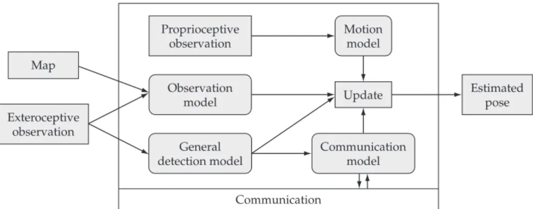
A single robot needs a map of environment and proprio-ceptive and exteroproprio-ceptive observations to be able to localize itself. All information gathered by the robot is fused with motion and observation model resulting in an estimated pose. Considering multiple robots, besides the information for single robot, the robots can use information communi-cated by other robots. A model for multirobot probabilistic localization is shown at Figure 1, the model includes general detection and communication models. All information about detections are communicated to other robots, through communication model, and used to update the robots poses beliefs.
The model for multirobot probabilistic localization consider the following assumptions:
• Initialrobots’posesareunknown. • Robotsknowanenvironmentmodel.
• Robotsareequippedwithproprioceptivesensorsthat measure their own motion.
for each pose x do
Initialize p(x0 = x)
end for loop
if robot receives an odometer reading then for each pose x do
p(xt = x) =
x’
∑
p(xt= x|xt−1 = x’,at−1)p(xt−1 = x’)end for end if
if robot receives a sensor reading then for each pose x do
p(xt = x) = p(ot|xt= x)p(xt = x)
∑
x’p(ot|xt = x’)p(xt = x’)
• Robotsareequippedwithexteroceptivesensorsthat monitor the environment, and detect and identify other robots.
• Robots are equipped with the same communication devices that allow them to exchange information. The communication model deals with the messages exchanged among robots and the synchronization of the robots at the moments of updating poses beliefs.
The General Detection Model – GDM uses useful informa-tion provided by robots of the group to update robots pose beliefs. The main information obtained is detection, however, some variants of detection can also be used:
• Positivedetection,whenarobotdetectsanotherone and measures its relative distance;
• Absence of detection, or negative detection, that provides the information about places where a robot cannot be;
• Multidetection, when a detection occurs involving more than a pair of robots. It implies ways to update poses of all robots involved in detection, and
• Propagationofadetectionfornonparticipantsrobots, that similar with the absence of detection, provides information about places where a robot cannot be. The aim of this paper is to describe general detection model. All the components for general detection model, beginning with detection between a pair of robots, are described in next sections.
3.1. Positive detection model
The positive detection model or only detection model6 is based on the assumption that each robot is able to detect and identify another robot and furthermore, the robots can communicate their probabilities distributions to other robots. Let’s suppose that robot n detects robot m, m ≠ n, and that it measures the relative distance between them, so:
n n
t t 1
n m m
t 1 t 1 n t 1
x
p(
= x) = p(
= x)
p(
= x|
= x , )p(
= x ),
−
− − −
′
∑
′
′
x
x
x
x
r
x
(3)where
x
nt represents the pose of robot n,x
mtrepresents the pose of robot m and rn denotes the measured distance between robots. The calculation
n m m
x′
p(
t 1−= x|
t 1−= x , )p(
n t 1−= x )
∑
x
x
′
r
x
′
describes the beliefof robot m over the pose of robot n. Similarly, the same detec-tion is used to update the pose of robot m.
Once a detection is made according to the detec-tion model, the two robots involved in the process share their probabilities distributions and relative distance. This communication significantly improves the localization accu-racy, when compared to a less communicative localization approach. The multirobot localization algorithm proposed by Fox et al.2 presents the advantage of performing global localization. Robots in the group cooperate to find their poses, communicating their poses beliefs when they meet.
3.2. Negative detection model
The aim of negative detection model is to show how negative information can be incorporated in multirobot localization8. The idea is that even a failed attempt to detect a robot is a useful information, which can be used to improve localization accuracy.
Negative information measurement means that at a given time, the sensor is expected to report a measurement but it did not. Most of the techniques of state estimation use a sensor model that update the state belief when the sensor reports a measurement. However it is possible to get useful information of the state from the absence of sensor measure-ments relative to the expected measurement landmarks.
Human beings often use negative information. For example, if you are looking for someone in a house, and you do not see the person in a room, you can use this nega-tive information as an evidence that the person is not in that room, so you should look for him/her in another place.
In the cooperative multirobot localization problem negative information can also mean the absence of detec-tions (in the case that a robot does not detect another one), which configures a lack of group information. In this case, the negative detection measurement can provide the useful information that a robot is not located in the visibility area of another robot. In some cases, it can be an essential
infor-Communication Proprioceptive
observation
Estimated pose Map
Exteroceptive observation
Observation model
Communication model General
detection model
Motion model
Update
mation as it could improve the pose belief of a robot that is located at a part of environment with few discriminant land-marks.
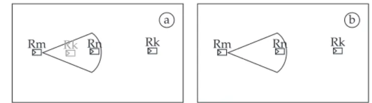
Consider two robots within a known environment and their field of view as shown in Figure 2a. If robot 1 does not detect robot 2 at a given point in time, a negative information is reported, which states that robot 2 is not in the visibility area of robot 1.
The information gathered from Figure 2a is true if we consider that there are no occlusions. In order to account for occlusions it is necessary to sense the environment to identify free areas or occupied areas. If there is a free space on the visibility area of a detection sensor, than there is not an occlusion. Otherwise, if it is identified as an occupied area it means that the other robot could be occluded by another robot or an obstacle. In this case it is possible to use geometric inference to determine which part of the visi-bility area can be used as negative detection information, as shown in Figure 2b.
Let’s suppose that robot m makes a negative detection. The negative detection model, considering the visibility area of the robot and the occlusion area, becomes:
m m
m t t t
t m m
t t t
x
p(
|
= x, ,
)p(
= x)
p(
= x) =
,
p(
|
= x , ,
)p(
= x )
− −
− ′
∑
′
′
d
x
v obs
x
x
d
x
v obs
x
(4)where
d
t− is the event of not detecting any robot and xm corresponds to the state of robot m, the robot that reports the negative detection information. The variables v and obs represent the visibility area and the identified obstacles, respectively.Whenever a robot m does not detect another robot k, we can update the probability distribution function of each k, with k ≠ m, in the following way:
k m
k t t
t k m
t t
x
p(
= x)p(
= x)
p(
= x) =
,
p(
= x )p(
= x )
−
− ′
∑
′
′
x
x
x
x
x
(5)where xk, for k = 0, …, n, represents all robots which were not detected.
Negative detection model allows solving certain localiza-tion problems that are unsolvable for a group of robots that only relies on positive detection information. A typical situa-tion is the case of robots in different rooms, in a way that one robot cannot detect the other.
3.3. Detection propagation model
In this section it is explained the detection propagation model6. In this model, all the robots in a group (bigger than two robots) can benefit from the shared information derived from a single detection (when robot m meets robot n).
Suppose a robot k in the group in doubt of being in two different poses as shown in Figure 3a. When robot m meets robot n, robot k can conclude that it is not in the robot m and n poses, once only one robot can occupy the same space in the environment at the same time. Robot k can also conclude that it is not in the way between the two meeting robots, otherwise, robot m would have detected robot k instead of robot n, as depicted in Figure 3b.
It is supposed that the detection sensor can sense robots in front of it. For example, the detection sensor could be a camera (pointing forward) to identify the robot and a prox-imity sensor to measure the distance.
The information from the two meeting robots can be prop-agated to the other robots in the group. It can be performed by the robot m, that realizes the detection. When robot n updates its pose with the information communicated by robot m, it communicates back its updated probability distribution. Robot m then calculates a probability distribution that will be communicated to the non-meeting robots:
k m
d t t
m n n
t t t
p (
= x ) = 1 (p(
= x )
p(
= x ,
= x) p(
= x)),
−
+
′′
′
+
′
x
x
x
x
x
(6)where
p (
dx
kt= x )
′′
is the information communicated to thenon-meeting robots,
p(
x
mt= x )
′
is the probabilitydistribu-tion of robot m,
p(
x
nt= x)
is the probability distribution of robot n andp(
x
mt= x ,
′
x
nt= x)
is the probability distribu-tion of a robot being in the way between the two meeting robots.Robot k can update its pose belief using the following equation:
k k
k d t t
t k k
d t t
x
p (
= x)p(
= x)
p(
= x) =
.
p (
= x )p(
= x )
′
∑
′
′
x
x
x
x
x
(7)Detection propagation model is an useful information for robots non participants of detection. It is worth to mention that the information from propagation of detection cannot be obtained with negative detection.
Robot 1
Robot 2
a b
Figure 2. a) Robot field of view. b) Occlusion in the field of view.
Rm Rk Rn Rk Rm Rn Rk
a b
3.4. Multidetection model
In this section it is described the multidetection model7, which is the problem posed when a robot participates in a detection that involves more than a pair of robots at the same time as illustrated in Figure 4. In order to solve this problem we present a multidetection model, which is an extension of the previous detection model proposed by Fox et al.2. The key idea here is to explore the best way to exchange information between robots when they meet, keeping the communica-tion requirements as minimal as possible, and increasing the localization accuracy.
The key idea is that robots with more certainty about their poses have more useful information to share with other robots, so they should communicate first, propagating their knowledge to the rest of the group.
We use the entropy value, defined by Shannon14 to measure the robot’s uncertainty of its pose:
t t
x
H =
−
∑p(
x
= x)log p(
x
= x),
(8)where p(xt = x) denotes the robot’s belief that it is at pose x. This belief represents a probability distribution over all the space of xt. In this way, entropy value H is used as an informa-tion theoretical quality measure of the pose estimainforma-tion. The entropy of p(xt = x) approximates zero if the robot is perfectly localized, and reaches a maximum value when p(xt = x) is uniformly distributed.
It is therefore necessary to define the uncertainty measure for two meeting robots instead of only one. Thus, the infor-mation gained from the meeting of two robots is given by the maximum value of entropy between the robots, as follows:
ij i j
H = max(H , H ),
(9)where Hij represents the entropy value of a meeting between robots Ri and Rj.
Suppose a group of robots taking part in a multidetec-tion configuramultidetec-tion. This configuramultidetec-tion can be represented by a graph G = (V, E), where V is the set of nodes and E is the set of directed edges. Let each robot be represented as a node, and each detection be represented as a directed edge, linking the two meeting robots, pointing to the detected robot. In this way, the configuration that each robot detects all the others can be represented as a complete directed graph. All edges (Ri, Rj) in E are labeled by a weighted value that corresponds to the entropy Hij.
If the graph presents bidirectional edges it means that two robots are detecting and being detected by each other at the same time. In this case, two types of robots should be considered: 1) homogeneous or 2) heterogeneous, regarding their exteroceptive sensors capabilities, i.e., the error intro-duced in their relative distance measures. In the first case, we just eliminate one direction of the bidirectional edge; in the latter, we just keep the direction pointing to the less accurate robot, i.e., the sensor reading from the most accurate sensor will be used to update the robots’ poses beliefs.
Given a weighted graph G, the multidetection problem can be formulated as finding a subset of edges E’ from E, in a manner that all nodes of V are incidents on edges in E’, and G = (V, E’) has the minimum total weight.
At any moment it is possible to represent the detection configuration of the robots by a graph G = (V, E). Given G, the following should be performed in order to update robots’ poses:
• Reduceallbidirectionaledgestounidirectionalones. • Weighteachedge(Ri, Rj) by Hij.
• Chooseasubsetofedges
E
′
⊂
E
, so that G = (V, E’) has the minimum weight.• SorttheedgesofE’bytheirminimumweight. • Updaterobots’beliefsfollowingtherankededgesofE’. Following this it is possible to find the detection update order to deal with multidetection, in a way that minimize the communication requirements, obtaining as much informa-tion as possible with all detecinforma-tions identified.
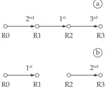
As an example, consider the robot configuration depicted by Figure 4. What is the update order that obtains the best information gain? If we suppose the minimum entropy values for the meetings are, in order,(R1, R2), (R0, R1) and (R2, R3), then, the update order should be (R1, R2), (R0, R1) and (R2, R3). So, each pair of robots updates their poses beliefs using Equation 3, following the order presented, as shown in Figure 4a. Now, suppose that the minimum entropy values for the meetings are, in order, (R0, R1), (R2, R3) and (R1, R2), then, the update order is (R0, R1) and (R2, R3) and each robot updates its pose belief using Equation 3, as can be seen in Figure 4b. It is worth noting that in this case it is not necessary to update (R1, R2), once R1 is already updated in (R0, R1) and R2 in (R2, R3).
3.4.1. Computationally tractable representation
The multirobot localization is based on the idea that in absence of detections (positive, negative or multidetection) each robot performs Markov localization independently. When a detection occurs, the robots involved in the meeting update their poses beliefs, refining their local estimates. Thus, the multirobot localization is based on a factorial representation, as it assumes that the distribution of all robots’ poses is the product of its marginal distributions. For a group of n robots:
1 n 1 n
t t t t
p( ,
x
,
x
|d) = p( |d). .p(
x
x
|d),
(10)where d is all data gathered by the robots, it includes envi-ronment, movement and detection measurements. Once the
2nd 1st 3rd
R0 R1 R2 R3 a
1st 2nd
R0 R1 R2 R3 b
Figure 4. Poses beliefs update order: a) 1st: (R1, R2), 2nd: (R0, R1), and
robots share their poses beliefs, the independence assumption does not hold. For example, when robot R1 meets R2, robot R1 updates its pose belief using the pose belief of robot R2, which means that
p( ) = p( |
x
1tx
1tx
2t)
, so independence assumptiondoes not hold, once the distribution of all robots’ poses is not the product of its marginal distribution. Thus, the factored representation is an approximation of the true distribution.
The factorial representation has the advantage that the pose estimation is carried out locally on each robot, which means a computationally tractable representation, once the computation of the join distribution of the poses of all robots is infeasible.
The risk in representing the join distribution
1 n
t t
p( ,
x
,
x
,|d)
as an approximated factored distribution is that repeated approximations may cause errors growing unboundedly over time. To reduce this risk, Fox et al.2 included a counter that, once a robot has been detected, it blocks the ability to see the same robot again until the detecting robot has traveled a pre-defined distance. Experimentally this approach showed to be sufficient. Confirming that, Boyen and Koller1 show that the stochasticity of the process serves to attenuate the effects of errors over time, fast enough to prevent the accumulated errors from growing unboundedly.Thus, the multidetection technique proposed in Section 3.4 is an approximated factored representation of the true probability distribution, but as stated by Fox et al.2 and Boyen & Koller1, the errors introduced do not lead the poses estimation to diverge.
Another problem with multidetection update occurs when one robot uses the same evidence to update its pose more than once, for example, when R0 detects R1, R1 detects R2, and R2 detects R0, if R0 and R1 update their poses beliefs, followed by R1 and R2, when R2 and R1 update their poses beliefs, R0 will receive twice the information from R1. This kind of update can easily lead to over-convergence, with pose estimates converging to some precise but inaccurate value. To avoid this, the update detection structure proposed in 3.4 stops the update when each node is visited, i.e., when all robots have their poses updated.
4. Multirobot Markov Localization
In the multirobot Markov localization each robot updates its pose belief whenever a new information is available: motion information; environment observation; detection among robots; propagation of detection to non participants robots and negative detection. It can be seen in Algorithm 2.
5. Experiments
In order to evaluate the localization results obtained with general detection model proposed in this paper we perform some experiments, comparing our approach to a previous approach based on positive detections2. The experiments are performed in simulated environment, where each robot is equipped with a proximity sensor to measure the distance to the walls in the environment, and a detection sensor, that can identify other robots and measure their relative distance. All robot sensors are assumed to be corrupted by Gaussian noise and robots know an environment model.
for each robot x ndo 0
n
0 for each pose x do
Initialize p(x = x)
end for end for loop
for each robot x do
if robot receives an odometer reading then for each pose x do
p(x = t x) = n
x’
∑
p(x = x|x = x’,a )p(x = x’)end for end if
if robot receives a sensor reading then for each pose x do
p(x = x) =
∑
x’p(o |x = x’)p(x = x’) end forend if
if robot n participates in a detection then for each pair of detection in which robot n participates
do
for each pose x do
p(x = x)= p(x = x’)
x’
∑
p(x = x|x = x’,rn)p(x = x’)end for end for end if
if robot n receives propagation of detection from robot
m then
for each pose x do
p(x = x) = pd(x = x)p(x = x)
∑x’
pd(x = x’)p(x = x’)end for end if
if robot n receives negative detection from robot m then
for each pose x do
end for end if end for end loop n t n t n t−1 n t−1 n t−1 n t n t n t n t
∑x’
p(x = m- x’)p(x = x’) tn t
p(x = m- x)p(x = x) t n t n t n t n t
p(x = n x) = t n t-1 n t-1 m t-1 m t-1 n t n t n t
p(o |x = n x)p(x = x) t
n t n
t
Algorithm 2. Multirobot Markov Localization with Generalized Detection Model
In the first part of the experiments the negative detec-tion model, detecdetec-tion propagadetec-tion model and multidetecdetec-tion model are tested separately. The environment used for these tests is an opened area. The environment has dimensions 3.2 × 2.0 meters. The robot environment model is a grid-based model, where each cell has dimensions of 0.2 × 0.2 meters, and angular resolution of 90 degrees. It results in a state space of dimension 16 × 10 × 4 = 640 states.
5.1. Experiment with negative detection model
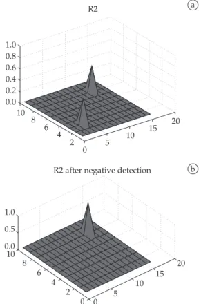
We conducted a preliminary experiment with three robots. At a given moment, robot 1 knows accurately its pose, as shown in Figure 5a. Robots 2 and 3 are in doubt about being in two places as shown in Figures 6a and 7a.
Considering that each robot cannot detect the others and environment observations are not enough to disambiguate between possible poses of robots in doubt, it should be impossible to robot 2 and 3 to find out their real poses alone at that moment.
However, robot 2 would be able to localize itself if negative detection information from robot 1 could be used to update its pose belief. In Figure 5b is shown the negative detection information derived from the belief of robot 1 and its visi-bility area. When robot 2 updates its pose using the negative detection information reported by robot 1, it becomes certain about its pose, as shown in Figure 6b. The same occurs with robot 3, as shown in Figure 7b.
If negative detection model was not used, robots 2 and 3 should walk around, waiting to detect or to be detected by a robot certain about its pose or until they find out useful landmarks at the environment. In this way, negative detec-tion provides the ability to localize robots more quickly, compared with positive detection.
0 2 4 6 8 10
5 10
15 20
0 0 2 4 6 8 10 0.0 1.0 0.5
5 10
15 20 0.0
0.5 1.0
R1 a
Negative information of R1 b
Figure 5. Experiment with negative detection model: a) Initial poses beliefs for Robot 1. b) Negative information from Robot 1.
a
b 1.0
0.8 0.6 0.4 0.2 0.0
10 8
6 4
2
0 5
10 15 20
1.0 0.5 0.0 10
8 6
4 2
0 0 5
10 15
20 R2 after negative detection
R2
Figure 6. Experiment with negative detection model: a) Initial poses beliefs for Robot 2. b) Robot 2 after negative detection.
a
b 0.0
10 8
6 4
2 0 0.2
0.4 0.6 0.8 1.0
5 10
15 20 R3
10 0.0 0.5 1.0
8 6
4 2
0 0 5
10 15
20 R3 after negative detection
5.2. Experiment with detection propagation model
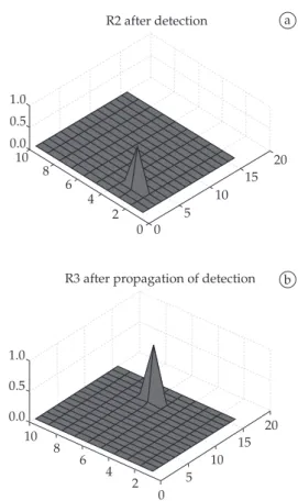
The detection propagation model was tested with three robots. At a given moment, robot 1 knows accurately its pose, as shown in Figure 8a. Robots 2 and 3 are in doubt about being in two places as shown in Figures 8b and 8c.
If robot 1 detects robot 2, using positive detection model, robot 2 becomes certain about its pose, as shown in Figure 9a, and robot 3 keeps its previous pose knowledge. Robot 3 would have to walk around, wait until it find out useful landmarks at the environment or to be part of a positive detection.
However, if detection propagation model is available, the information of the detection from robot 1 and 2 is shared with robot 3, then it becomes certain about its pose, because the possibility of being between robot 1 and robot 2 is eliminated as illustrated in Figure 9b.
R1
0.0 0.5 1.0
10 8
6 4
2
0 5
10 15
20
10 8
6 4
2 0
5 10
15 20 0.0
0.5 1.0
10 8
6 4
2 0
5 10
15 20 0.0
0.2 0.4 0.6 0.8 1.0
R3 R2
a
b
c
Figure 8. Experiment with detection propagation model: Initial poses beliefs for a) Robot 1. b) Robot 2. c) Robot 3.
a
b 10
0.0 0.5 1.0
8 6
4 2
0 0 5
10 15
20 R2 after detection
0.0 0.5 1.0
10 8
6 4
2 0
5 10
15 20 R3 after propagation of detection
Figure 9. Experiment with detection propagation model: Robot 1 detects robot 2. a) Poses belief for robot 2 after detection. b) Poses beliefs for robot 3 after propagation of detection.
R1 R2
R3 R4
Figure 10. Configuration of the four robots.
The experiment shows the improvement in cooperative multirobot localization obtained if a detection informa-tion is propagated for all robots in the group. The detecinforma-tion propagation model allows better localization results than in positive detection2.
5.3. Experiment with multidetection model
0.4 0.2 0.0
10 8
6 4
2 0
5 10
15 20 R1
10 0.0 0.5 1.0
8 6
4 2
0 0 5
10 15
20 R2
a
b
Figure 11. Experiment with multidetection model: Initial poses beliefs for a) Robot 1. b) Robot 2.
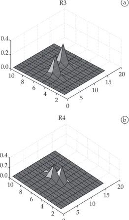
0.0 10
8 6
4 2
0 5
10 15
20 0.2
0.4
R3
0.0 10
8 6
4 2
0 5
10 15
20 0.2
0.4
R4
a
b
Figure 12. Experiment with multidetection model: Initial poses beliefs for a) Robot 3. b) Robot 4.
With the same setup described above, we tested the locali-zation results obtained with: 1) positive detection model2 and 2) our proposed multidetection model.
The positive detection model first updates poses beliefs of robots 1 and 2, resulting in a new accurate pose belief for robot 1 as shown at Figure 13a, and robot 1 and robot 2 cannot participate in other detection at this moment. The next update is from robot 3 with robot 4, resulting in poses beliefs that do not improve localization accuracy of these robots, as shown at Figures 13b and 13c. As all robots have taken part of detections, i.e., robot 1 with 2 and robot 3 with 4, there is no more updates to be done.
10 0.0 0.5 1.0
8 6
4 2
0 5
10 15
20
0 5
10 15
20
2 4 6 8 10 0.0 0.2 0.4
10 0.0 0.2 0.4
8 6
4 2
0 5
10 15
20 R4 after detection
R1 after detection
R3 after detection
a
b
c
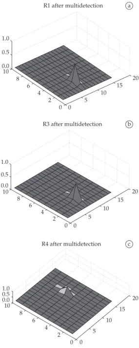
The multidetection model represents detection situation by a graph with four nodes, R1, R2, R3 e R4 and four edges, (R1, R2), (R2, R3), (R3, R4) and (R4, R1). Each edge is labeled by a weighted value that corresponds to the entropy H12, H23, H34 and H41, respectively. The edges are sorted as follows: (R1, R2), (R2, R3) and (R4, R1). The edge (R3, R4) is removed from the graph because R3 has been already updated in (R2, R3) and R4 in (R4, R1).
The results of the poses belief after the updates can be seen at Figures 14a, 14b and 14c. We can see that multide-tection model allows all robots to improve their pose beliefs differently from single detection where only one of the robots improve its belief.
5.4. Experiment with general detection model
The experiment was conducted in the environment shown in Figure 15, it is a symmetric environment with two similar rooms, three smaller similar rooms and four corri-dors. The environment has dimensions 9.2 × 6.6 meters. The robot environment model is a grid-based model, where each cell has dimensions of 0.2 × 0.2 meters, and angular resolu-tion of 90 degrees. It results in a state space of dimension 46 × 33 × 4 = 6072 states.
We perform tests with a group of twelve robots assuming the configuration depicted in Figure 15, where some of the robots know its initial pose and others do not as follows:
• Robots1,3and7knowaccuratelytheirposes. • Robots4,10and12areindoubtabouttwopossible
poses.
• Robot2isindoubtaboutthreepossibleposes. • Allotherrobotsarecompletelyuncertainabouttheir
poses.
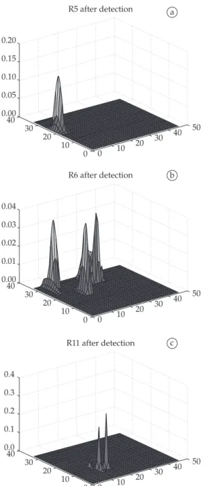
The situations of doubt are doubled marked in Figure 15. The experiment conducted with detection model performed the following updates: robot 3 with 5, robot 6 with 7, robot 8 with 9 and robot 10 with 11. The improvements obtained with the detections can be seen at Figures 17a, 17b and 17c for robots 5, 6 and 11, respectively.
The experiment conducted with general detection model can be seen at Figure 16, that shows the graph representing
10 8
6 4
2 0 0
5 10
15 20 0.0
0.5 1.0
10 0.0 0.5 1.0
8 6
4 2
0 0 5
10 15
20
10 0.0 0.5 1.0
8 6
4 2
0 0 5
10 15
20 R4 after multidetection
R3 after multidetection
R1 after multidetection a
b
c
R1
R6
R4
R7 R8 R2 R11
R10 R3
R5
R9
R12 R12
R4
R9
R2 R2
R11
R12 R3
R5
R9 R8
R7 R6
R10
Figure 14. Experiment with multidetection model: a) Robot 1 after multidetection. b) Robot 3 after multidetection. c) Robot 4 after multidetection.
Figure 15. Experiment environment.
40 30
20 10
0 0 10
20 30
40 50 0.00
0.05 0.10 0.15 0.20
R5 after detection a
40 30
20 10
0 0 10
20 30
40 50 0.00
0.01 0.02 0.03 0.04
R6 after detection b
40 30
20 10
0 0 10
20 30
40 50 0.0
0.1 0.2 0.3 0.4
R11 after detection c
Figure 17. Experiment with positive detection model: a) Robot 5 after detection. b) Robot 6 after detection. c) Robot 11 after detection.
40 30
20 10
0 0 10
20 30
40 50 0.00
0.05 0.10 0.15 0.20
R5 after multidetection a
40 30
20 10
0 0 10
20 30
40 50 0.0
0.1 0.2 0.3 0.4
R8 after multidetection b
40 30
20 10
0 0 10
20 30
40 50 0.0
0.1 0.2 0.3 0.4
R8 after multidetection c
Figure 18. Experiment with general detection model: a) Robot 5 after detection. b) Robot 6 after detection. c) Robot 8 after detection.
the detections occurring in the experiment. The order of update considering entropy values of the edges is: (R10, R12), (R7, R8), (R3, R5), (R11, R12), (R8, R9) and (R6, R7).
The resulting poses beliefs after multidetection can be seen at Figures 18a, 18b, 18c, 19a, 19b, 20a and 20b.
Detection from robot 3 to robot 5 can be propagated to robot 4, as shown at Figure 21a and negative detection from R1 improves pose beliefs of robot 2, as shown at Figure 21b.
In the experiment conducted, general detection model outperforms positive detection allowing more accurate localization results, as expected. Moreover, the integration of
techniques in GDM enables better localization results than the application of each technique separately, as follow:
• Positive detection improves beliefs of robots 5, 6 and 11.
• Multidetection improves beliefs of robots 5, 6, 8, 9, 10, 11 and 12.
• Propagationofdetectionimprovesbeliefofrobot4. • Negativedetectionimprovesbeliefofrobot2. • GDM improves beliefs of robots 2, 4, 5, 6, 8, 9, 10,
6. Experiment with Real Robots
Soccer competitions, such as RoboCup12, has been proven to be an important challenge domain for research, where localization techniques have been widely used. The experi-ments in this work were conducted in the domain of the RoboCup Standard Platform Four-Legged League, using the 2006 rules10,9. In this domain, two teams consisting of four Sony AIBO robots compete in a color-coded field: the carpet is green, the lines are white, the goals are yellow and blue. Cylindrical beacons are placed on the edge of the field at 1/4 and 3/4 of the length of the field. Considering only the white lines on the floor, that are symmetric, the field, shown in Figure 22, has dimensions 5.4 × 3.6 meters. The robot environment model is based on a grid, where each cell has dimensions of 0.3 × 0.3 meters, and angular resolu-tion of 90 degrees. It results in a state space of dimension 18 × 12 × 4 = 864 states.
The robots used in this experiment were the Sony Aibo ERS-7M3, a 576MHz MIPS R7000 based robot with 64 Mb of RAM, 802.11b wireless Ethernet and dimensions of 180 × 278 × 319 mm. Each robot is equipped with a CMOS color camera, X, Y, and Z accelerometers and 3 IR distance sensors that can be used to measure the distance to the walls in the environment.
The 416 × 320 pixel nose-mounted camera, which has a field of vision 56.9° wide and 45.2° high, is used as a
detec-40 30
20 10
0 0 10
20 30
40 50 0.00
0.05 0.10 0.15 0.25 0.20
R9 after multidetection a
40 30
20 10
0 0 10
20 30
40 50 0.0
0.2 0.4 0.6 1.0 0.8
R10 after multidetection b
Figure 19. Experiment with general detection model: a) Robot 9 after multidetection. b) Robot 10 after multidetection.
40 30
20 10
0 0 10
20 30
40 50
0.0 0.2 0.4 0.6 0.8
R11 after multidetection a
40 30
20 10
0 0 10
20 30
40 50
0.0 0.2 0.4 0.6 1.0
0.8
R12 after multidetection b
Figure 20. Experiment with general detection model: a) Robot 11 after multidetection. b) Robot 12 after multidetection.
a
b 40
30 20
10
0 0 10
20 30
40 50 0.0
0.2 0.4 0.6 0.8
R4 after propagation of detection
40 30
20 10
0 0 10
20 30
40 50 0.0
0.1 0.2 0.3 0.5 0.4
R2 after negative detection
tion sensor. In order to verify if there are any robots in the image and to measure their relative distance, we used the constellation method proposed by Lowe, together with its interest point detector and descriptor SIFT5.
In this domain, there are situations in which the robots are not able to detect the color markers, such as the beacons or the goals (corner situations, for example). In these moments, only the lines are visible, and the robots must cooperate to over-come the difficulties found by the symmetry of the field.
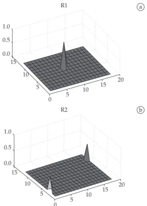
We conducted an experiment with two robots. Robot 1 is located at the center of the field facing the yellow goal. At a given moment, robot 1 knows accurately its pose, and robot 2 is in doubt about being at the yellow goal area or at blue goal area of the field. Figure 22 depicts this situation. Due to the environment symmetry it is impossible to robot 2 to find out that its real pose is in the blue goal area of the field, considering that the colored marks, goals or beacons, are not in its field of view, as can be seen in Figure 23b. However, robot 2 would be able to localize itself if negative detection information, provided by robot 1, could be used to update its pose belief.
Figures 24a and 24b show the probability density function of robot 1 and robot 2, respectively. In Figure 25a is shown the negative detection information derived from the belief of robot 1 and its visibility area. When robot 2 updates its pose using the negative detection information reported by robot 1, it becomes certain about its pose, as shown in Figure 25b.
Robot 2
Robot 2
Robot 1 Robot 1
a
b
Figure 22. Experiment: robot 1 at the center of the field and two possible positions of robot 2.
a b
Figure 23. Images from the robot cameras: a) Image seen by robot 1. b) Image seen by robot 2.
15 10
5
0 5
10 15 20
15 10
5
0 5
10 15 20 R1
R2 0.0
0.5 1.0
0.0 0.5 1.0
a
b
Figure 24. a) Probability density function of robot 1. b) Probability density function of robot 2.
7. Conclusions
We have presented a cooperative multirobot localization based on Markov localization. The novelty of the paper is the general detection model that uses diversified information to update robots poses as: detection involving two or more robots, propagation of detection for non participants robots and absence of detections.
The experimental results presented have demonstrated that our approach, when compared to a previous multirobot localization method, reduces the uncertainty in localization significantly and provide the ability to localize robots more quickly. These are highly beneficial in real world applications where robots need to actually perform a task rather than to localize perfectly.
it. In this way, we give a contribution in the direction of a precise localization, that is one of the main requirements for mobile robot autonomy.
A limitation of our work is the increase in the amount of data needed to communicate in order to update robots’ poses. Thus, in future work, we are interested in exploring the tradeoff between communication and localization accu-racy.
Another point to be explored is active detection. It means that when a robot knows its pose it can communicate it to all the robots within the group, and they can look for the right robot in order to communicate with it and improve their poses beliefs.
Acknowlegdements
This research has been conducted under the FAPESP Project LogProb (Grant No. 2008/03995-5) and the CNPq Project Ob-SLAM (Grant No. 475690/2008-7). Anna H. R. Costa is grateful to CNPq (Grant No. 305512/2008-0). Reinaldo Bianchi also acknowledge the support of the CNPq (Grant No. 201591/2007-3).
References
1. Boyen X and Koller D. Tractable inference for complex stochastic processes. In: Proceedings of the Fourteenth Annual Conference on Uncertainty in Artificial Intelligence; 1998; Madison, Wisconsin. San Francisco: Morgan Kaufmann; 1998. p. 33-42.
2. Fox D, Burgard W, Kruppa H and Thrun S. A probabilistic approach to collaborative multi-robot localization.
Autonomous Robots 2000; 8(3): 325–344.
3. Fox D, Burgard W and Thrun S. Markov localization for mobile robots in dynamic environments. Journal of Artificial Intelligence Research 1999; 11:391-427.
4. Howard A, Mataric M and Sukhatme G. Putting the “i” in “team”: an egocentric approach to cooperative localization. In: Proceedings of IEEE International Conference on Robotics and Automation; 2000; Taipei, Taiwan. New York: Kluwer Academic Publishers; 2003. p. 14-19.
5. Leonard J and Durrant-Whyte H. Mobile robot localization by tracking geometric beacons. IEEE Transactions on Robotics and Automation 1991; 7(3):376-382.
6. Lima PU. Bayesian approach to sensor fusion in autonomous sensor and robot networks. IEEE Instrumentation and Measurement Magazine 2007; 10(3):22-17.
7. Lowe D. Distinctive image features from scale invariant keypoints. International Journal of Computer Vision 2004; 60(2):91-110.
8. Odakura V and Costa AHR. Cooperative multi-robot localization: using communication to reduce localization error. In: Proceedings of International Conference on Informatics in Control, Automation and Robotics; 2005; Barcelona. Portugal: INSTICC Press; 2005. p. 88-93.
9. Odakura V and Costa AHR. Multidetection in multirobot cooperative localization. In: Proceedings of First IFAC Workshop on Multivehicle Systems; 2006; Salvador. São José dos Campos: Instituto Tecnológico de Aeronáutica (Biblioteca Central); 2006. p. 19-24.
10. Odakura V and Costa AHR. Negative information in cooperative multirobot localization. In: Proceedings of Advances in Artificial Intelligence; 2006; Ribeirão Preto, São Paulo. New York: Springer; 2006. p. 552-561. (v. LNAI 4140). 11. Odakura V, Sacchi R, Ramisa A, Bianchi R and Costa AHR.
The use of negative detection in cooperative localization in a team of four-legged robots. In: Anais do Simpósio Brasileiro de Automação Inteligente; 2009; Brasília. Porto Alegre: SBA; 2009.
12. RoboCup Technical Committee. RoboCup Four-Legged League Rule Book. Switzerland: The RoboCup Federation; 2006. 13. Roumeliotis SI and Bekey GA. Distributed multirobot
localization. IEEE Transactions on Robotics and Automation
2002; 18(2):781-795.
14. Russell S and Norvig P. Artificial Intelligence: a modern approach. New Jersey: Prentice Hall; 1995.
Figure 25. a) Negative detection information reported by robot 1. b) Probability density function of robot 2 after the incorporation of negative detection information.
a
b 15
10 5
0 0 5 10
15 20 0.0
0.5 1.0
15 10
5
0 5
10 15 20 0.0
0.5 1.0