J. Braz. Comp. Soc. vol.15 número3

*e-mail: prestes@inf.ufrgs.br

An improved particle filter for sparse environments

Edson Prestes*, Marcus Ritt, Gustavo Führ

Instituto de Informática – UFRGS, P.O. Box 15064, 91501-970, Porto Alegre, RS, Brazil

Received: July 7, 2009; Accepted: August 27, 2009

Abstract: In this paper, we combine a path planner based on Boundary Value Problems (BVP) and Monte Carlo Localization (MCL) to solve the wake-up robot problem in a sparse environment. This problem is difficult since large regions of sparse environments do not provide relevant information for the robot to recover its pose. We propose a novel method that distributes particle poses only in relevant parts of the environment and leads the robot along these regions using the numeric solution of a BVP. Several experiments show that the improved method leads to a better initial particle distribution and a better convergence of the localization process.

Keywords: boundary value problems, autonomous navigation, environment exploration, global localization, Monte Carlo localization.

1. Introduction

The localization process is an essential component of any mobile robotic system during a navigation task in the envi-ronment. It endows the robot with the capacity to determine its correct pose using the collected sensory data. This capacity is considered as a prerequisite to make a robot really autono-mous. One of the basic problems in localization is position tracking that corresponds to a local localization problem and aims to estimate actively the robot’s pose (x, y, q) from a known initial pose. It tries to compensate for noise in the sensors and errors in odometric readings that can arise in a systematic or non-systematic way to determine the most likely world pose.

Local localization techniques are particularly impor-tant during the exploration and building of environment maps. They enable the generation of a faithful representa-tion of the environment while minimizing or eliminating the mapping distortion produced by odometric errors. The task of mapping and simultaneously self-localizing is diffi-cult, because the robot needs to determine its pose based on a map that is being currently built and to map precisely the environment using the information on its pose. This problem is called Simultaneous Localization and Mapping (SLAM) and has attracted the attention of several researchers during last years21,3,2,4_.

Besides the position tracking problem, there are other challenging localization problems like the kidnapped robot problem and the wake-up robot problem. They comprise a class of global localization problems. In the wake-up problem, the robot must determine its pose without prior knowledge about its initial location. In the kidnapped robot problem, a well-localized robot is carried to another position during its navigation without being told. In both problems, global local-ization techniques must be able to handle multiple candidate poses at same time.

Most of the methods used for local localization are unable to solve global localization problems. The main reason is that global localization demands to track and to analyze multiple hypotheses simultaneously. For instance, methods for posi-tion tracking based on Kalman filtering24,17 _{represent the}

robot’s estimated pose using an unimodal Gaussian distri-bution, where the distribution mode provides the current robot position and the variance is the accuracy of the estima-tion. This distribution limits the use of Kalman filters when there are several candidate poses. To circumvent this, Jensfelt and Kristensen14 _{propose a probabilistic approach that uses}

multiple hypotheses to represent the robot pose. These hypotheses are updated according to the observation made by robot sensors. The hypothesis corresponding to the true robot pose will be more distinguishable than false hypoth-eses.

The most common approach to handle both global and local localization is the particle filter28_{. The algorithms based}

on particles belong to a class of methods known as Monte Carlo Localization (MCL). MCL algorithms are easily imple-mented and computationally efficient since they focus the search on certain regions in the space with high likelihood to contain the real robot pose. There are lots of variations of the basic algorithm. For instance, Milstein et al.19 _{suggest the use}

of clusters of particles to handle symmetric environments. They claim that the basic algorithm converges quickly to a single high probability pose even if there are more than two similar likely poses. Kwon et al.16 _{minimize the number of}

samples used in MCL using topological information about the environment. This information aims to determine where the particles should be placed in the environment. In this case, the particles are drawn around the neighborhood of the topological edges reducing the number of particles and augmenting the algorithms’ efficiency. Gasparri et al.12 _propose

clustering method to handle the global localization problem. At each resampling step, the robot executes a dynamical clustering and at each time step, it executes an evolutionary action to find out the local maxima within each cluster.

In this paper, we propose a strategy that combines path planning based on boundary value problems (BVP) and MCL to solve the global localization problem in large and sparse environments. This problem is difficult since large parts of this kind of environment do not provide relevant structural information for the robot to recover its pose. We propose a method that puts particles only in relevant parts of the envi-ronment and leads the robot along relevant regions using the numeric solution of a BVP. The main differences between our proposal compared to Coastal Navigation23 _{are that in}

our case the robot’s initial pose is unknown and our strategy takes advantage of the environment structure as a cue to particle generation.

This paper is organized as follows. Sections 2 and 3 present the Monte Carlo Localization and the BVP-path planner, respectively. Section 4 introduces the method proposed to draw particles using BVP and in Section 5 we present an experimental evaluation of the new approach. Finally, Section 6 presents our conclusions.

2. Monte Carlo Localization

Monte Carlo Localization is a class of algorithms that computes a robot’s pose using a Bayesian approach and the assumption that the environment is Markovian. Basically, the posterior densities (beliefs), Bel (S_t), over the robot state S_t at instant t, are computed using the sensor data and odometric data in a recursive way through

(1)

where h is a normalization constant, o_t is the sensor measure gathered during the robot movement at time t and at-1 is the

odometric data associated to the robot motion between the instants t–1 and t. The probability p(s_t | s_t-1, a_t-1) is associated to the probabilistic model of the robot motion and p(o_t | s_t) is the probabilistic observation model. Both models assume a Gaussian distribution with zero mean.

To compute Equation 1 is not a simple task. The main problem is the computational requirements to calculate Bel(s) over the space of possible poses. To alleviate this problem, Thrun27 _{developed a particle filtering that uses only a fraction}

of samples drawn from the poses space.

The filtering represents the beliefs by a set of m samples

i i m

t t t i=1

S = {s , w }

where each sample represents a particular pose si _{= (x, y,} q_{) and the w}i _{are non-negative importance}

factors, which sum up to one. The algorithm starts drawing m samples using the initial knowledge about the candi-date robot poses given by S₀. The initial importance factor of each sample is equal to 1/m, that is, all the samples are equiprobable to be the correct robot pose. Recursively, the new generations of samples are determined according to the steps below

1. Resampling: Sample

s

it 1− from the sample set

repre-senting

S

t 1− according to the weights

w

it 1− .

2. Sampling: The odometric data are used to deter-mine the estimated robot pose,

s

i_t, at instant t, using

− −

i

t t 1 t 1

p(s |s

, a

)

.

3. Importance sampling: The sample importance wi _is

evaluated using

w = p(o |s )

i

η

t it .

3. Path Planner Based on Boundary Value

Problems

Recently, we proposed a framework for controlling a robot in navigational tasks, like the exploration of unknown environments and the planning of paths between known positions6,7,29,22,8_{. It is based on potential fields that do not have}

local minima generated through the numeric solution of the BVP using Dirichlet boundary conditions and the following equation

∇

2

_p(r)

+ ε ⋅∇

_v

_{p(r) = 0}

₍₂₎

where v is a bias vector and e฀is a scalar value. The allowed values of the parameters e and v generate an expressive amount of action sequences that the robot can take to reach a specific target (goal position) or to explore an unknown environment. Basically, the method discretizes the environ-ment into a fixed homogeneous mesh with identical cells, like an occupancy grid. Each cell (i, j) is associated to a squared region of the real environment and possesses a potential value p_i,j. Dirichlet boundary conditions are such that the cells with high probability of having an obstacle are set to potential 1 (high) while cells containing the target are set to potential 0 (low).

In the exploratory tasks, the robot collects information on the obstacles using its sensor and updates the mesh cells. We consider the unknown regions as targets that the robot must reach then the unknown regions cells are assigned to a low potential value (see Prestes et al.22 _{and Trevisan et al.}29

for more information). By using this information, the Gauss-Seidel algorithm is employed to update the potential cells according to

− + − +

+ − + −

+

+

+

+

ε

−

+

−

i, j i 1, j i 1, j i, j 1 i, j 1

i 1, j i 1, j x i, j 1 i, j 1 y

1

p = (p

p

p

p

)

4

((p

p

)v

(p

p

)v )

8

(3)

where v = (v_x, v_y) and

ε ∈ − +

[ 2, 2]

. The robot uses the gradient descent of this potential to determine the path to follow towards the target position. This method is formally complete, i.e., if there is a path connecting the robot posi-tion to the target, it will be found. The high potential value prevents the robot from running into obstacles whereas the low potential value generates an attraction basin that pulls the robot.

extend our strategy to incorporate environmental features. They can be used as good clues to orient the exploration of an unknown environment and to construct routes between locations of interest25_{. By selecting different features in}

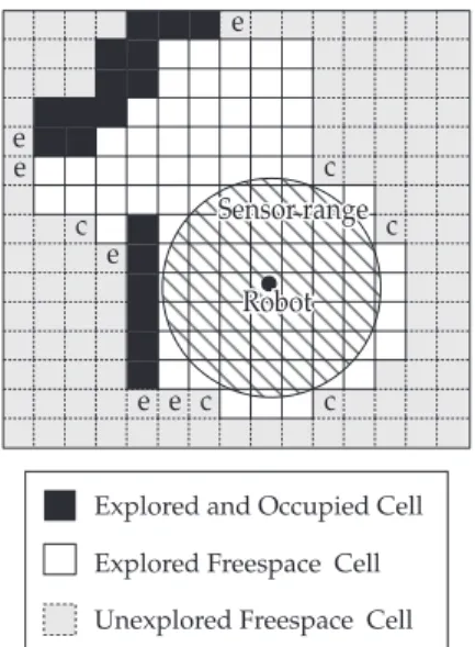
the boundaries we can generate different strategies for the complete exploration of the environment. These strate-gies are associated with the potential values attributed to the different boundary configurations used to calculate the potential in Equation 2. For example, consider the environ-ment represented in Figure 1. Regions labeled as “e” are edges of walls. When the robot explores these regions first it should exhibit a wall-following behavior. But if the robot avoids the walls seeking to fill unexplored concave regions, like the ones labeled as “c”, it should exhibit a space-filling behavior.

As we stated above, the behavior of the robot is given by the boundary conditions, where the boundary is held at a potential defined by some function along the boundary, i.e.,

∈∂Γ

p( ) = f( ) for

r

r

r

(4)

where ∂G฀is the borderline between the explored and unex-plored space of the environment G. Wall-following exploring behavior is achieved just setting a low potential (f(r) = 0) in wall edges and their neighborhood. On the other hand, space-filling exploring behavior is achieved setting low potential in unexplored concave regions.

4. Particle Selection Based on BVP

A standard particle filter draws samples uniformly at random from the environment free-space. This process has some disadvantages for localization. First, the process can demand a high number of particles to completely cover the environment in order to guarantee that the robot will be able

to recover its pose. It is known that the performance of the Monte Carlo filter highly depends on having some particles with a pose close to the real robot pose in the initial distribu-tion10_{. Second, all regions of the environment have the same}

a priori probability to contain the robot pose. In large open regions, the absence of structural information makes the system spend a lot of time processing irrelevant particles, that is, particles which cannot contribute to determine the robot pose, since the robot will only be able to localize itself when its sensors capture some information from obstacles. Third, the regions near the obstacles are in general improp-erly covered with a low particle density that can not represent adequately the real robot pose. Taking these problems into consideration, a better solution is to distribute the particles near obstacles instead of distributing them uniformly over all the environment. To make such a strategy effective, it requires a robust algorithm that leads the robot preferentially along the obstacles while guaranteeing the exploration of the complete environment.

An approach to solve these problems has been proposed by Tae-Bum Kwon16_{. They suggest to distribute the particles}

along the edges of the environment’s topological map. As these edges represent only a fraction of the environment, the method will process a smaller set of particles, thus reducing the computational cost. To localize itself, the robot initially explores the local environment until reaching an edge of the topological map, and afterwards navigates on the edges of the topological map15_{. The particles’ belief is updated only}

during this second phase.

Kwon et al.’s method is very adequate when the robot is inserted in a dense environment. As the edges correspond to the middle of the corridors, the robot will navigate the environment always sensing the obstacles around. However in a sparse environment, the edges will conduct the robot through an area where it will not be able to sense any obstacle. Particles on topological edges contribute no information in sparse environments due to the absence of structural infor-mation. Then, the method will fail because this area does not have any relevant information that can help the robot to recover its pose.

Our approach solves these problems using a combina-tion of an exploracombina-tion based on the solucombina-tion of a BVP22,9,29

and a variation of the skeletization algorithm used in image processing13_{. For localization, the robot first explores the}

environment until sensing an obstacle. We then use the inter-mediate results of the skeletization algorithm on the global map to determine relevant parts of the environment which represent all the positions where the robot can sense any obstacle. Afterwards we use the solution of a BVP defined on the skeleton and the global map to generate an initial distribution of the particles. Then, the robot continues the exploration, preferentially following obstacles, using our exploration method described in Section 3.

This approach has several advantages. First, the poten-tial produced by the BVP focuses the particle distribution on regions more probable to contain the robot’s real pose avoiding large open regions. Second, the BVP does not e

e

e c

c c

e

e e c c

Explored and Occupied Cell

Explored Freespace Cell

Unexplored Freespace Cell

Sensor range Sensor range

Robot Robot

constrain the robot movement through the middle of corri-dors (or topological edges), which is not adequate in a sparse environment. The robot will explore, for instance, the envi-ronment following walls as long as possible but switch to explore open regions if necessary. Therefore our method can be applied to any kind of environment.

Our proposal can be viewed as an integrated explora-tion strategy11,5,26,18_{, since the robot is guided to regions that}

contain information to minimize the uncertainty about its pose. Strategies like this tend to produce better results than purely random strategies, since they use additional informa-tion about the environment to determine the best next acinforma-tion to be executed. They differ mainly in the way they determine the region that must be visited, which can be chosen using a cost function. Amigoni1 _{shows that strategies that use cost}

functions to reach a balance between exploration and precision in mapping tend to be more efficient than random or greedy exploration strategies. As the environment used in the experi-ment is sparse, regions near obstacles are more important than the others becoming more attractive to the robot. Then, our approach will lead the robot to the relevant environment region, instead of the regions that represent a sparse area.

The following sections describe our method in detail. Section 4.1 shows how we use skeletization and BVP to find a better initial distribution of the particles. In Section 4.2 we show how we can use the knowledge about the exploration behavior of the robot to further improve the distribution of the initial direction of the particles.

4.1. Extracting the intermediary environment skeleton

Our method determines the cells that the robot will prob-ably visit during its navigation using the intermediary result of a skeletization process. Skeletization is a morphological thinning used in binary images that successively erodes away pixels from the boundary until no more thinning is possible. At the end, the pixels left over correspond to the image skel-eton. In our case, the erosion acts on the free-space cells and at each erosion step, also called relaxation step, the free-space is shrunk at most one cell from its boundary.

If we want to guarantee that the robot always receives sensor readings, we must constrain it to navigate always at a maximum distance drobot from the obstacles. Depending

on the environment, the robot can navigate always at a distance drobot. However, the robot may need to visit a

narrow corridor with width less than d_robot. Then the cells that should be visited comprise the intermediary result of the skeletization process after r relaxation steps, where

r

=

_d

robot/wcell and wcell is the grid cell width. Even if the

robot enters in a corridor with width less than 2drobot, the

visited cells will be identified by this method. These cells, called visiting cells, are marked and receive a potential value of 0.5. The value 0.5 has been chosen to indicate good navi-gation positions and because the potential values vary in interval [0,1]. Obstacles have a potential value of 1 and cells near the sparse regions have a potential of 0. The skeletiza-tion process is continued for another r steps and the cells,

called border cells, that represent the new intermediary skel-eton have their potential values set to 0. Then, the harmonic potential of the other cells in the free-space is computed.

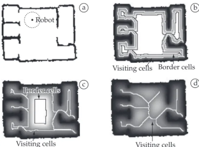
Figure 2a shows a sparse environment, the robot (solid black circle) and its view field (dashed circle). We can see that the robot can observe only a small fraction of the environment at a time. Figure 2b shows the potential field and the visiting and border cells generated using our approach. It also shows in gray scale the cells potential value, where the black and white correspond to the potential 1 and 0, respectively. The white cells have a potential value of 0 and a distance of 2d_robot or more from the obstacles. In this case, the radius of robot vision field is 2drobot. Hence, the white cells represent positions

where the robot will not sense any obstacle. Figure 2c shows the results if we double drobot in comparison to the experiment

shown in Figure 2b. Figure 2d shows the skeleton extracted after the complete convergence of the skeletization algorithm.

To generate the initial particle distribution, we use the potential value of each cell to determine its prob-ability to be selected to receive particles. Consider that we want to put k particles at a cell r = (i, j). The equation

−

−

2

Pr(r is selected) = exp( c(p(r) 0.5) )

(5)

provides the probability that each one of the k particles will be generated at space region related to the cell r, where p(r) is the potential of the cell r and c is a constant that determines what cells around the skeleton will be used to draw the parti-cles based on their potential values. The smaller the constant value the more cells near the skeleton will have high prob-ability to receive particles.

The advantage of using the solution of a BVP to deter-mine the cells’ potential is that this method adapts itself to any kind of environment and produces a linear distribution of the potential from the obstacles.

Robot

a

c

b

d

Visiting cells

Visiting cells

Visiting cells Border cells

Border cells

Border cells

4.2. Using the potential to improve filter convergence

The BVP method allows us to further improve the initial distribution of the particles. Consider the initial phase of the exploration and localization. When the robot starts in a sparse region of the environment, where it cannot sense any obstacle, the BVP path planner will generate a space-filling behavior to explore this open region, until an obstacle is found. Then, the robot will determine its orientation and shows a wall-fol-lowing behavior, moving perpendicular to the gradient of the current potential field. When encountering the first obstacle, the initial distribution of the particles is generated according to the method described in the previous section. We can improve the likelihood of producing good initial positions taking into consideration the robot’s orientation. Since it will follow walls in this phase, particles with orientation perpendicular to the gradient of the global vector field are more likely to repre-sent the robot’s actual orientation. We therefore distribute the particle orientations uniformly over all directions which do no deviate more than a maximum angle f from a direction perpen-dicular to the vector field. The angle f allows to compensate errors due to measurement and incomplete information of the robot’s local map. In our experiments, f = 30° has shown to produce good results (see section 5.4 below). Figure 3 shows an example of the particle distribution according to this method.

5. Experiments

This section presents several experiments conducted using the simulator MobileSim (version 0.4.0) of the robot Pioneer 3DX.20_{. In Subsection 5.1, we give examples of the typical}

behaviour of the global localization process in environments of different density and connectivity. Afterwards, we present the results of three experiments. In a first, preparatory experiment, we compare the ability of the uniform distribution, Kwon et al.’s method and our method based on potential fields to distribute the particles in regions with high relevance for the localization process. The second experiment compares the quality of the localization of the three initial particle distributions. The third experiment studies the improvement of convergence using the method of Section 4.2 to distribute the initial orientation of the particles, according to the robot’s orientation. In all experiments, d_robot is equal to half of the radius of the robot vision field.

Robot

a b

Figure 3. Initial distribution of particles according to initial direction of the robot. a) Global distribution of the particles and the robot’s pose after determining its initial orientation. b) Detailed view of the particles’ distribution in the region highlighted in (a).

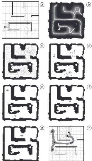
Figure 4. Example of a successful localization in environment A. a) Map of the environment. b) Potential field (in grey) used to define the initial particle distribution. c)-g) Particle distribution when the robot is at positions 1-5 and simulation steps 1, 11, 21, 60, 76, respec-tively, as shown in (h).

5.1. Global localization in environments of different

density

In this subsection, we give three examples of a global localization process using our method based on BVPs for the exploration combined with the improved initial particle distri-bution described in Section 4. We compare the behavior of the method in environments of different density, as shown in Figures 4a, 5a, and 6a. Environment A is dense, environment B sparse, but with a connected boundary and environment C sparse and non-connected. The environments have been chosen to verify that our method can be applied to any kind of environment, including sparse and non-connected ones, where a simple wall-following strategy will fail to explore the complete environment. The three environments have different sizes and grid cell widths as shown in Table 1.

In all three environments, we try to localize the robot, where it can sense any obstacle at a maximum distance of 2 m. The initial potential field and the resulting initial particle distribution are shown in Figures 4b, 5b, 6b.

a

c

e

g h

b

d

f

1 2 3

1 2 3

4

5 6 i

a

c

e

g h

b

d

f

Figure 5. Example of a successful localization in environment B. a) Map of the environment. b) Potential field (in grey) used to define the initial particle distribution. c)-h) Particles distribution when the robot is at positions 1-6 and simulation steps 1, 14, 20, 26, 39, 65 respectively, as shown in i.

Table 1. Characteristics of the three environments used in the experi-ments.

Type Size [m]

Cell size [cm]

r

A Dense 10 × 10 10 × 10 10

B Sparse, connected 30 × 24 24 × 24 4

C Sparse, unconnected 26 × 20 24 × 24 4

a

c

e

g

i

h b

d

f

1 2 3

4 5 6

Figure 6. Example of a successful localization in environment C. a) Map of the environment. b) Potential field (in grey) used to define the initial particle distribution. c)-h) Particle distribution when the robot is at positions 1-6 and simulation steps 2, 38, 65, 95, 108, 183, respectively, as shown in i.

For environment A, Figures 4c-g show the particle distri-bution when the robot is at positions 1-5, respectively, as shown in Figure 4h. The path followed by the robot during the process is the curve in Figure 4h. For environment B, Figures 5c-h illustrate the convergence of the particles to a limited region in the environment. The path followed by the robot during the process is the curve in Figure 5i. For

envi-ronment C, Figures 6c-h show the distribution of the particles when the robot is at positions 1-6, respectively, as shown in Figure 6i. The path followed by the robot during the process is the curve in Figure 6i.

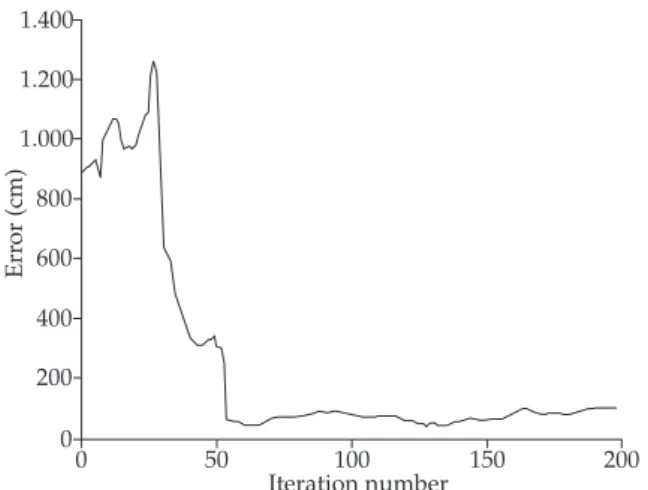
Figure 7 shows a typical example of the evolution of the localization error during the localization process in environ-ment C. The localization error is calculated as the difference between the predicted position of the robot and the actual position in the simulator. The error tends to decrease according to the data acquired by the robot and stay bounded near to zero. In this case, the localization error is bounded by 96 cm which corresponds to four times of the environment’s cell size.

The magnitude of the localization error in our experi-ments stems from two main sources:

1. _{The robot maintains a discrete map of the}

the expected sensor reading of a particle can be deter-mined to a precision of at best one cell size.

2. To determine the true localization error in the simu-lation, we have to map the current position estimate of the robot’s position, into the simulator’s coordinate system. This is done using a linear transformation. It can cause an additional, artificial error, if the robot’s map contains non-linearities introduced during the initial exploration.

For this reason, in the following experiments, we consider a localization trial being successful, if the final localization error is less than four times the map’s cell size. Observe that the error introduced by the discretization can be decreased by reducing the cell size during exploration, at a higher processing cost.

5.2. Experiment 1: Comparison of the initial particle

distribution of the three methods

With this preparatory experiment we want to verify that our method produces good environment coverage when compared to the uniform distribution and the topo-logical distribution. To this aim, we focus this experiment on the particle distribution generated by each method, more precisely, in the amount of selected cells that will contain the particles instead of the amount of particles per cell. So, we consider that each free-space cell can be selected or not to contain just one particle.

The uniform distribution selects a free-space cell with probability 0.5. The topological distribution selects cells that comprise the environment’s topological map or neighboring cells up to a distance of two cells with probability 0.5. Our method chooses a cell based on its potential value using Equation 5 and c = 20, that is, the cells with potential values in the interval [0.4, 0.6] are more likely to be used to draw the particles.

The experiments have been conducted in the environ-ment shown in Figure 2a since it contains sparse and dense regions depending on the robot’s field of vision. If the robot’s

field of vision is small, then the environment is completely sparse, otherwise it can be dense inside the rooms and sparse in the center, or dense everywhere.

To compare the resulting particle distributions, we deter-mine the amount of free-space cells that can provide sensor information, to help the robot to recover its pose. Figure 8 shows an example of the cells selected using the three methods. The cells in Figure 8a have been selected using the uniform distribution, while the cells in Figure 8b and Figure 8c have been selected using our method and the topo-logical distribution, respectively. Considering that the robot has a small field of vision, as shown in Figure 2a, we can see that most of cells selected by the uniform distribution and the topological distribution will be placed in the center of the environment. On the other hand, our method selects the cells near the robot that are more likely to correspond to the real robot pose.

These observations are confirmed by the following exper-iment. We subdivide the real environment of approximately 30 × 24 m into grid cells of size 24 × 24 cm. We consider that the robot navigates at maximum distance d_robot from the obsta-cles and that the radius of vision field is 2drobot. The distance

drobot has been varied from 50 cm up to 2.5 m, in increments

of 25 cm. For each value cells relevant for localization are at maximum distance 2drobot from the obstacles, since cells more

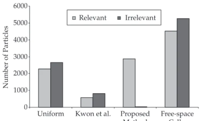
distant than this comprise the sparse region of the environ-ment. The environment has in average over different fields of vision 4520 relevant cells and 5250 irrelevant cells.

A comparison of the three methods is shown in Figure 9. The uniform distribution selected in average 2260 relevant particles and 2650 irrelevant ones. The relevant cells corre-spond to ≈43% of relevant free-space cells. The topological distribution selected in average 571 relevant particles and 821 irrelevant ones. The relevant cells correspond to ≈12% of relevant free-space cells. Our method selected ≈63% of the relevant free-space cells and only 0.3% of irrelevant cells. The processing using our method focuses just on the regions that can contribute for the robot to recover its pose.

1.400

1.200

1.000

800

600

400

200

0

0 50 100 150 200

Err

or (cm)

Iteration number

Figure 7. Example of an evolution of the localization error in envi-ronment C.

a

c

b

In conclusion, our method is able to generate an initial particle distribution which almost entirely consists of posi-tions relevant for the localization of the robot. This leads to a higher convergence rate, as the following experiments show.

5.3. Experiment 2: Influence of the initial distribution

on the convergence

In this set of experiments we compare the convergence of the Monte Carlo filter for different initial particle distri-butions, where the particle orientation is random. The experiments have been conducted in the environment shown in Figure 6a. This environment is challenging for a global localization, since it is sparse, non-connected and has several symmetries.

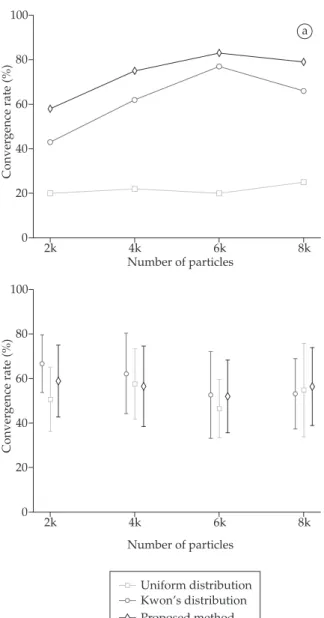
In each experiment we generated 50 different initial posi-tions of the robot. For each position we try to localize the robot using the uniform distribution, the topological distri-bution and our method, with sample sizes of 2000, 4000, 6000 and 8000 particles. Each localization trial has been run for 150 time steps. A trial is considered to be successful, when the difference between the predicted and actual robot position is less than 96 cm (four times the cell size) at the end of the run. A trial which did not converge in this time frame is consid-ered a failure. Figure 10a and Table 2 show the convergence rate, i.e. the number of successful localizations, as a function of the number of particles and the initial particle distribu-tion.

The chosen environment is large and sparse, and there-fore the probability of generating an initial particle close to the true position of the robot is small. Since, the perform-ance of the Monte Carlo filter highly depends on this (see the discussion in section 4), we observe low overall convergence rates between 10 and 66%. As expected, the convergence rate increases with the number of particles for all three initial distributions. The proposed method performs better than the other distributions, with 11 to 46% more successful local-izations. In particular, it obtains with 4 k particles a better convergence rates than the uniform distribution with 8 k particles.

Table 2. Percentage of successful localizations. For each initial particle distribution and number of particles the convergence rate over 50 trials without and with orientation of the particles is given.

Without orientation

Number of particles

Distribution 2 k 4 k 6 k 8 k

Uniform 18% 22% 45% 50%

Topological 10% 20% 16% 20%

Our method 43% 58% 56% 66%

With orientation

Number of particles

Distribution 2 k 4 k 6 k 8 k

Uniform 43% 62% 77% 66%

Topological 20% 22% 20% 25%

Our method 58% 75% 83% 79%

0 1000 2000 3000 4000 5000 6000

Uniform Free-space

Cells Relevant Irrelevant

Number of Particles

Kwon et al. Proposed Method

Figure 9. Comparison of relevant and irrelevant particles selected by different methods.

Figure 10. Results of localization experiments for different initial particle distributions and different numbers of particles. a) Percentage of successful localizations. b) Localization error of successful localizations.

100

80

60

40

20

0

2k 4k 6k 8k

Uniform distribution Kwon’s distribution Proposed method

Number of particles

a

100

80

60

40

20

0

2k 4k 6k 8k

Uniform distribution Kwon’s distribution Proposed method

Number of particles

Localization err

or (cm)

5.4. Experiment 3: Influence of the improved initial

orientation of the particles

In this set of experiment we study the convergence rate when distributing the orientation according to the known initial orientation of the robot as described in Section 4.2, and compare it to the strategy of the previous experiment, which distributes the orientation uniformly over all possible angles. The experimental setup is the same as in the previous experiment: we report averages over 50 trials, for each initial particle distribution, and samples sizes of 2.000, 4.000, 6.000 and 8.000 particles. All experiments have been conducted in the environment shown in Figure 6a choosing the robot’s initial pose randomly.

From the results shown in Figure 11 and Table 2 we can see that the use of the vector field significantly improves the convergence rate of the particle filter. The main reason is that it adds information on the expected robot pose during the localization process instead of using random particles with low likelihood of being a real robot pose. Generating the particles without regarding the expected robot behavior is to produce useless particles that will tend to rapidly disappear and will not contribute to the localization only increasing the processing cost. For instance, our method, using the vector field allows the filter to converge with 4000 particles in 75% of the trials (Figure 11a). Without using the information about the initial orientation, the standard Monte Carlo filter with uniform initial distribution achieves only a convergence rate of 66% with twice the number of particles (Figure 10a).

As in the previous experiment, we performed one additional evaluation with 20 k particles to verifiy the convergence of the methods. For both, the uniform and the proposed method, we obtained a convergence rate of 85% in this experiment.

6. Conclusions

In this paper, we propose a strategy that combines a path planner based on boundary value problems and MCL to solve the global localization problem in sparse environments. The proposed method has the advantage, that the poten-tial produced by the BVP focuses the particle distribution on regions more probable to contain the robot pose avoiding large open regions. Furthermore, the BVP path planner does not constrain the robot’s motion through the middle of corridors and can be used in dense as well as sparse environments. The localization driven by the solution of a BVP on the environment guides the robot along its significant parts. Our experiments show, that we can make a better use of the knowledge about the initial position in the environment extracted from the potential than the particle filter alone, improving the convergence rate about 10 to 20% in a sparse environment. The localization is precise up to about four times the resolution of the underlying grid. This allows to achieve the same convergence rates and localization errors using fewer particles.

For future work, we intend to deal with symmetric environ-ments and to use the information collected on the environment to determine where the robot must explore in order to minimize the odometric errors and produce a trustful environment map.

100

80

60

40

20

0

2k 4k 6k 8k

Number of particles

Conver

gence rate (%)

a

100

80

60

40

20

0

2k 4k 6k 8k

Number of particles

Conver

gence rate (%)

Uniform distribution Kwon’s distribution Proposed method

Figure 11. Results of localization experiments for different initial particle distributions and different numbers of particles. The parti-cle’s initial orientation is distributed using the orthogonal vector field according to the method proposed in Section 4. a) Percentage of successful localizations. b) Localization error of successful localiza-tions.

The average final localization error of the successful local-izations is shown in Figure 10b. For all three methods, and independent of the number of particles, a successful locali-zation leads to an average localilocali-zation error of about 63 cm equivalent to 2.6 cells, with a standard deviation of less than one cell width.

Acknowledgements

This work has been partially supported by Conselho Nacional de Desenvolvimento Científico e Tecnológico (CNPq), projects no. 620132/2008-6 and 481292/2008-0.

References

1. Amigoni F. Experimental evaluation of some exploration strategies for mobile robots. In: Proceedings of IEEE International Conference on Robotics and Automation; 2008; Pasadena, California. EUA: IEEE; 2008.

2. Angeli A, Doncieux S, Meyer JA and Filliat D. Incremental vision-based topological SLAM. In: Proceedingsof IEEE/RSJ International Conference on Intelligent Robots and Systems; 2008; Nice, França. EUA: IEEE; 2008.

3. Begum M, Mann GKI and Gosine RG. Concurrent mapping and localization for mobile robot using soft computing techniques. In: Proceedingsof IEEE/RSJ International Conference on Intelligent Robots and Systems; 2005; Alberta. Canada:IEEE; 2005.

4. Blanco JL, Fernández-Madrigal JA and González J. Efficient probabilistic range-only SLAM. In: Proceedingsof IEEE/RSJ International Conference on Intelligent Robots and Systems; 2008; Nice, França. EUA: IEEE; 2008.

5. Bourgault F, Makarenko AA, Williams SB, Grocholsky B and Durrant-Whyte HF. Information based adaptive robotic exploration. In: Proceedingsof IEEE/RSJ International Conference on Intelligent Robots and Systems; 2002. Switzerland: IEEE; 2002. 6. Dapper F, Prestes E, Idiart MAP and Nedel LP. Simulating

pedestrian behavior with potential fields. In: Advances in Computer Graphics. New York: Springer; 2006. p. 324-335. (Lecture Notes in Computer Science, v. 4035).

7. Dapper F, Prestes E and Nedel LP. Generating steering behaviors for virtual humanoids using BVP control. In:

Advances in Computer Graphics. New York: Springer; 2007. (Lecture Notes in Computer Science)

8. Faria G, Prestes E, Idiart MAP and Romero RAF. Multi robot system based on boundary value problems. In: Proceedings of IEEE/RSJ International Conference on Intelligent Robots and Systems; 2006; Beijing, China. EUA: IEEE; 2006. p. 424-429. 9. Faria G, Romero RAF, Prestes E, and Idiart MAP. Comparing

harmonic functions and potential fields in the trajectory control of mobile robots. In: Proceedingsof IEEE Conference on Robotics, Automation and Mechatronics; 2004; Singapore. IEEE; 2004. p. 762-767. (v. 1).

10. Fox D, Thrun S, Dellaert F and Burgard W. Particle filters for mobile robot localization. In: Doucet A, Freitas JFG and Gordon NJ. (Eds.). Sequential Monte Carlo in practice. New York: Springer; 2001.

11. Freda L, Loiudice F and Oriolo G. A randomized method for integrated exploration. In: Proceedings of IEEE/RSJ International Conference on Intelligent Robots and Systems; 2006; Beijing, China. EUA: IEEE; 2006.

12. Gasparri A, Panzieri S, Pascucci F and Ulivi G. Monte carlo filter in mobile robotics localization: a clustered evolutionary point of view. Journal of Intelligent and Robotic Systems. 2006; 47(2):155-174.

13. Gonzalez R and Woods R. Digital image processing. Estados Unidos: Addison-Wesley Publishing Company; 1992.

14. Jensfelt P and Kristensen S. Active global localisation for a mobile robot using multiple hypothesis tracking. IEEE Transactions on Robotics and Automation. 2001; 17(5):748-760. 15. Kwon TB and Song JB. Thinning-based topological

exploration using position probability of topological nodes. In: Proceedingsof IEEE/RSJ International Conference on Intelligent Robots and Systems; 2006; Beijing, China. EUA: IEEE; 2006. 16. Kwon TB, Yang JH, Song JB and Chung W. Efficiency

improvement in Monte Carlo localization through topological information. In: Proceedings of IEEE/RSJ International Conference on Intelligent Robots and Systems; 2006; Beijing. China: IEEE; 2006. p. 424-429.

17. Leonard JJ and Durrant-Whyte HF. Directed sonar sensing for mobile robot navigation. Norwell: Kluwer Academic; 1992. 18. Leung C, Huang S and Dissanayake G. Active SLAM using

model predictive control and attractor based exploration. In:

Proceedingsof IEEE/RSJ International Conference on Intelligent Robots and Systems; 2006; Beijing, China. EUA: IEEE; 2006. 19. Milstein A, Sanchez JN and Williamson ET. Robust global

localization using clustered particle filtering. In: Proceedings of Innovative Applications of Artificial Intelligence; 2002; Edmonton, Canada. EUA: The AAAI Press; 2002. p. 581-586. 20. Mobile Robots. Mobilesim. [on the internet]. Available from

http://robots.mobilerobots.com/wiki/MobileSim. Access in 10/09/2009.

21. Montemerlo M, Thrun S, Koller D and Wegbreit B. Fast SLAM: A factored solution to the simultaneous localization and mapping problem. In: Proceedingsof Innovative Applications of Artificial Intelligence; 2002; Edmonton, Canada. EUA: The AAAI Press; 2002.

22. Silva-Junior EP, Engel PM, Trevisan M and Idiart MAP. Exploration method using harmonic functions. Robotics and Autonomous Systems. 2002; 40(1):25-42.

23. Roy N, Burgard W, Fox D and Thrun S. Coastal navigation: mobile robot navigation with uncertainty in dynamic environments. In: ProceedingsofIEEE International Conference on Robotics and Automation; 1999; Detroit. EUA: IEEE ; 1999. 24. Schiele B and Crowley JL. A comparison of position

estimation techniques using occupancy grids. In: Proceedings ofIEEE International Conference on Robotics and Automation; 1994; San Diego. EUA: IEEE; 1994.

25. Smith L and Husbands P. Visual landmark navigation through large-scale environments. In: Proceedingsof EPSRC/ BBSRC International Workshop on Biologically Inspired Robotics: The Legacy of W. Grey Walter; 2002; Bristol. Londres: The Royal Society; 2002. p. 272-279.

26. Stachniss C, Grisetti G and Burgard W. Information gain-based exploration using raoblackwellized particle filters. In: Proceedings of Robotics: Science and Systems; 2005; Massachusetts. Cambridge: The MIT Press; 2005.

27. Thrun S, Burgard W, Fox D and Dellaert F. Robust Monte Carlo localization for mobile robots. Artificial Intelligence. 2000; 128(1/2):99-141.

28. Thrun S, Burgard W and Fox D. Probabilistic Robotics. Cambridge: The MIT Press; 2005.

29. Trevisan, M, Idiart MAP, Prestes E and Engel PM. Exploratory navigation based on dynamic boundary value problems.