ISSN 0104-6500
*e-mail: [email protected]
Adaptive complementary filtering algorithm
for mobile robot localization
Armando Alves Neto*, Douglas Guimarães Macharet,
Víctor Costa da Silva Campos, Mario Fernando Montenegro Campos
Computer Vision and Robotic Laboratory – VeRLab, Department of Computer Science, Federal University of Minas Gerais – UFMG, Belo Horizonte, MG, Brazil
Received: June 30, 2009; Accepted: August 27, 2009
Abstract: As a mobile robot navigates through an indoor environment, the condition of the floor is of low (or no) relevance to its decisions. In an outdoor environment, however, terrain characteristics play a major role on the robot’s motion. Without an adequate assessment of terrain conditions and irregularities, the robot will be prone to major failures, since the environment conditions may greatly vary. As such, it may assume any orientation about the three axes of its reference frame, which leads to a full six degrees of freedom configuration. The added three degrees of freedom have a major bearing on position and velocity estimation due to higher time complexity of classical techniques such as Kalman filters and particle filters. This article presents an algorithm for localization of mobile robots based on the complementary filtering technique to estimate the localization and orientation, through the fusion of data from IMU, GPS and compass. The main advantages are the low complexity of implementation and the high quality of the results for the case of navigation in outdoor environments (uneven terrain). The results obtained through this system are compared positively with those obtained using more complex and time consuming classic techniques.
Keywords: complementary filtering, localization, outdoor navigation, mobile robots.
1. Introduction
Recent advances in the computational foundations of robotics have led to the development of new algorithms and efficient methodologies for tackling several fundamental problems in robotics. The sustained improvement in proc-essor performance and sensors technology have made it possible to build vehicles that are substantially autonomous and capable to accomplish a wide variety of tasks in real world. Much of the effort that has been invested to increase the ability of mobile robots to make their own decisions has gone into tackling the core issues of mobility, namely locali-zation and mapping, which are heavily dependent on data interpretation and fusion. Localization consists in estimating the mobile robot’s position and orientation with respect to a given inertial frame, is considered a very hard problem due to the inherent uncertainty and non determinism of the real world. Mapping is a related problem, which may be described as the task of building up a representation of the world based on sensor information.
While moving in an indoor environment, most of the time only the robot’s pose on the plane needs to be known. The pose may be specified by a configuration vector P→(t) = [x(t) y(t) ψ(t)]T, in which x and y represent the position of the robot’s center of gravity and ψ represents its bearing angle with respect to some inertial reference frame. The simplifying assumption in the general case is that the terrain traversed by the robot is horizontal and flat, and usually
pavement characteristics such as surface types, and other and anomalies are neglected. This, however, is not the case in outdoor environments, where the terrain's topography and surface types have a major bearing on the robots displace-ment and navigation, and should be carefully considered
This paper describes the use of a powerful, yet simple, precise and efficient technique known as CF10, 5 to tackle the localization problem for mobile robots navigating on uneven terrains in outdoor environments. For our discussion, we cluster the typical irregularities found in outdoor environ-ments into three classes:
• Depressionsandbumps; • Slopes;and
• Differenttypesofsurface(e.g.gravel,sand,asphalt, grass).
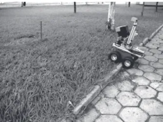
Figure 1 exemplifies the importance of having the full attitude information. It is shown the exact moment when the robot tranverses an obstacle, with a variation on its pitch angle. Without knowledge of this information the robot is more prone to failure, for example, navigating through a dangerous terrain without realizing it.
Several approaches have been reported in the literature, and in the next section the key ones will be presented and discussed.
2. Related Works
Several approaches for localization have been proposed in the robotics literature, and odometryI based techniques have been long used for that purpose. However, obtaining precise measurements from odometric sensors is very hard, for it is plagued with both sistematic and non-sistematic errors. In spite of all these drawbacks, odometry is widely used for navigation on planar, low slippage surfaces, which are prototypical of the majority of two dimensional indoor environments. Even in such controlled scenarios, odometric information alone becomes extremely limited if three-dimen-sional position and orientation need to be estimated, and this is typically the case in outdoor environments, where wheel slippage and attitude variations are more likely to happen.
One possible approach to overcome the problems present odometric measurements is to include other sensor modali-ties in the system, and combine all the acquired data in order to reduce uncertainties and thus to improve localization. This new set of sensors may or may not provide redundant infor-mation as far as the unknown variables are concerned. In general, one expects that as the number of sensors used to measure (directly or indirectly) a given variable increases, the confidence on the estimation increases .
Another type of sensor that has been widely used in robotic navigation and localization, mainly due to the reduction in cost of MEMS transducers, is the Inertial Measurement Unit IMU. This
I. Odometry is composed of two greek words: hodos (travel) and metron (measure), and consists in using data from actuators to estimate the robot’s displacement and its higher derivatives.
sensor is generally composed of gyros (angular velocity measure-ment devices) and acelerometers, orthogonally mounted on a base. The data produced by this type of sensor are usually corrupted with noise and bias, which are hard to deal with and demand careful filtering to minimize errors like those due to drift.
The literature brings many different solutions for high level processing and integration of sensor data. One example is described in Ojeda and Borestein12, where fuzzy logic is used in order to estimate the attitude of a mobile robot equipped with an IMU. However, the experiments presented in the paper showed results only for two dimensional, planar displacements, which disregards problems in extending the odometry information to the three-dimensional space (alti-tude information), common in systems that implements odometric and inertial data fusion.
In many cases, inertial navigation based systems perform sensor data fusion by means of a KF. Some examples can be found in Liu et al.9 and Sukkarieh13, where a system composed by an IMU and a GPS is shown. The fusion of data from the sensors was achieved by a standard KF, where system linearity was assumed. The joint use of IMU/GPS is described in Walchko and Mason16, where an EKF was used, and Li et al.8, where a SPKF was employed for data fusion purposes. In both cases, the filters are implementations of the KF for non-linear systems. The main difficulty associated with this method is the complexity in the identification of a good model for sensors and the robotic system. Another drawback is the high computational complexity of the solu-tion, which envolves intensive matrix manipulation.
A considerable number of solutions found in the literature is based on techniques for robots equipped with laser range scanners, which simultaneously to navigation, localize itself in the map of the environment it is concurrently building (SLAM). Information obtained from several sensors is then combined and used to correct the estimated position and orientation during navigation.
Müller and Surmann11 present a technique that is used by a large number of 3D SLAM works described in the litera-ture, which topically comprises of a laser scanner mounted on the robot facing the direction of displacement. In some implementations, the laser scanner is also able to rotate about its longitudinal axis. During data acquisition process, the robot moves a certain distance and then stops, at which moment, the laser scanner rotates to collect the information of a specific region. The newly acquired data are aligned with the previously collected ones, a process which improves the estimation of the robot’s current position. The main problems with this method are the use of an expensive sensor (laser scanner), and the associated computational complexity of the point registration algorithms.
In Thrun et al.15, the SLAM technique is used for the navigation of a helicopter model, where the computational complexity problem involved in mapping and localization is a key issue. However, one of the drawbacks of the presented solution is that it only works if the helicopter does not pass by the same place more than once, which is not easy to guar-antee as far as the robot’s motion is concerned.
21 Adaptive complementary filtering algorithm for mobile robot localization
Alternatively to the use of Kalman Filters for the data fusion, works based on other methodologies are also found in the literature. One such methodology is the CF, which allows the fusion of trustworthy signals with different frequency bandwidths to produce more precise signals in the time domain. This technique was used with success in aerial navi-gation as seen in Iscold et al.6, Baerveldt and Klang1, Euston et al.3 and Mahony and Hamel10. The main advantages of CF are the low computational cost, the faster dynamic response and the simplicity of parameter tuning.
3. Methodology
The method presented in this work is divided in two parts. On the first one, acceleration, angular velocity and magnetic orientation sensor signals are combined to generate an atti-tude estimate for the mobile robot in the three-dimensional space. On the second part, this attitude is used as part of the robot’s spatial position estimation, also considering the signals generated by a GPS receiver and the robot velocity odometry. In both parts, we use a methodology based on the CF princi-ples with cutt-off frequency adapted in function of the sensors characteristics, in order to generate better estimates of the robot’s configuration in the three-dimensional space.
3.1. Adaptive complementary filter algorithm
Before presenting a more detailed explanation of our methodology, we discuss the main idea of the algorithm used in this paper. This algorithm receives as input a set of data given by several sensors in the mobile robot, and provides as output the robot’s pose (position and orientation) in the three-dimensional space. As will be seen in the next sections, the technique has a low computational cost, which allows the use of the technique in real time (online, localization deter-mined while the robot navigates).
Firstly, we consider a mobile robot equipped with a set of sensors composed by three orthogonal accelerometers (a→), three orthogonal gyroscopes (g→), two orthogonal magnetometers (m→), an odometric sensor (v0), and a GPS receiver (x
→
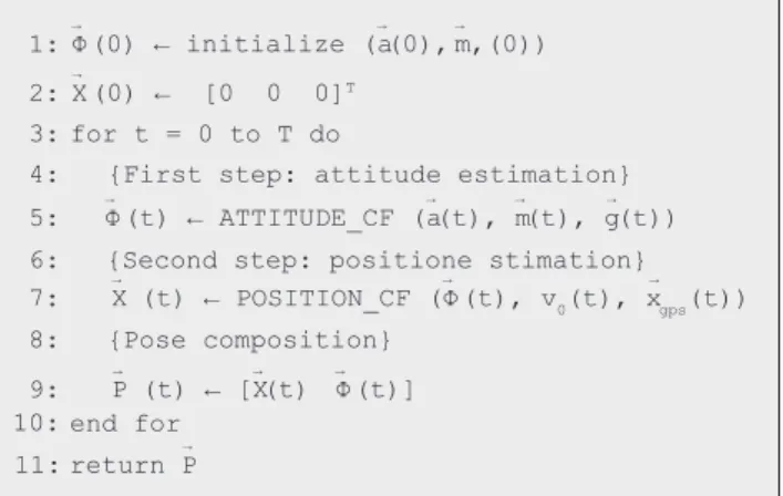
gps). The signals provided by these sensors are combined according to the Algorithm 1, which is divided in two fundamental parts.
On the first part, we use the a→, m→ and g→ signals to calcu-late an estimate of the orientation vector Φ→of the robot. This estimate is computed by the ATTITUDE_CF function, which implements an adaptive CF with variable cut-off frequency.
Similarly, on the second part, we use the angles Φ→ esti-mated on the previous step, the v0 value and the GPS signal to generate an estimate of the robot’s position X→. The adaptive CF computed by the POSITION_CF function is used to deal with problems such as sensor uncertainty and GPS signal loss.
This function and the previous one are explained in the following sections, as well as the initialization steps and the final pose vector (P→). For the sake of completeness, we describe the main caracteristics of each sensor used in each step, and use this information when dealing with the desing of the adaptive complementary filters. We also derive the computational complexity of this and and some other data fusion techniques.
3.2. Complementary filter for attitude estimation
In this section, we present the three main stages of the first part of the methodology. They encompass the design of the Adaptive CF for attitude estimation. Initially, the output of the accelerometers are used to produce a first estimate of the roll (φ) and pitch (θ) angles of the robot. Next, an estimate of the yaw (Ψ) angle is calculated. A second estimate of these three angles is generated through the integration of the signals from the three orthogonally mounted angular velocity sensors. On the last stage, these signals are fused to generate more reli-able estimates for the robot's pitch, roll and yaw angles. This fusion is made by means of complementary filters in which the cut-off frequency is adapted from some characteristics of the used sensors. This result is then used to estimate the spatial localization of the robot on a later part of the methodology.
3.2.1. Attitude estimation based on accelerometer
measurements
The measurement of the Earth’s gravity vector, by means of the three accelerometers that compose the IMU, is used to generate the first estimate of the robot’s attitude, considering only pitch (θ) and roll (φ) angles. These sensors are mounted along three orthogonal axes. We also assume the existence of a frame fixed to the Earth's plane, usually know as NED frame, as shown in Figure 2.
1:Φ→ (0) ← initialize (a→(0), m→,(0))
5: Φ→ (t) ← ATTITUDE_CF (a→(t), m→(t), g→(t))
7: X→ (t) ← POSITION_CF (Φ→ (t), v0(t), x→gps(t))
9: P→ (t) ← [X→(t) Φ→ (t)] 2: X→ (0) ← [0 0 0]T 3:for t = 0 to T do
4: {First step: attitude estimation}
8: {Pose composition}
6: {Second step: positione stimation}
10:end for 11:return P→
Algorithm 1. ADAPTIVE_CF (a→, m→, g→, v0, x
→
gps).
Z
g0 X
Y IMU
probot
X Y
NED Z
We know from the kinematic principles of rigid bodies that if we consider the NED frame as an inertial frame, the acceleration experienced by a point described by a vector r→a in relation to the robot’s center of mass (CM), and fixed to the robot’s body (e.g. the IMU) is given by
a CM a a
a = a
+ α × + ω × ω ×
r
(
r )
, where a→CM represents the acceleration of the robot’s center of mass, a→ is the angular acceleration of r→a , and ω→ is the angular velocity of this in the space.If we consider the use of a three axial sensor to measure this vector, we will also observe the effect of the gravity accel-eration of the Earth. In general, this effect is subtracted from the final result, in order to simplify the use of the IMU data. Equation 1 represents the values measured by the sensor. In this arrangement, it is possible to represent the gravity accel-eration vector as g→NED = [0 0 g
0]
T, which is constant in relation
to the Earth’s frame, and whose value is approximately g0≈9.78 m/s2.
ABC NED IMU a NED a
a
= a
R
( , , )g
−
φ θ ψ
+ ν
. (1)The gravity vector can also be described with respect to the IMU frame by multiplying g→NED by a rotation matrix
ABC
NEDRthat relates the two frames. However, in order to apply this rotation, it is necessary to compute this matrix or, in other words, to know what are the sensor’s orientation angles in space.
Another characteristic of the sensor is the uncertain parameter v→a which represents all noise involved in the process. Here, we use a single variable to express gaussian white noise, bias noise and imprecision due to the lack of orthogonality among the sensors.
To simplify the mathematics, it will be assumed that the IMU is mounted exactly on the robot’s center of gravity, which in the real case this may not necessarily be true. However, the chosen approach works well even if the difference between the actual location of the center of gravity and the sensor location is not very large. Therefore, we assume that the robot frame, ABC, and IMU frame, are coincident. We will also ignore all types of noise that corrupt the signals meas-ured in this case. These considerations alow us to simplify the previous equation to comply with Equation 2.
ABC NED IMU NED
a = a
=
R
( , , )g
−
φ θ ψ
. (2)Stripping the above matrix equation and rewriting the angles as functions of the projection of the vector a→IMU on each one of the IMU axes, it is possible to obtain estimates for φ and θ using the measurements from each of the accelerom-eters, as seen in equations 3 and 4.
x a
a
= arcsin
,
a
θ
(3)y a
a
a
= arcsin
,
a cos
φ
−
θ
(4)where ax and ay represent the components of the acceleration vector measured along the IMU X and Y axes.
It is important to note that a few assumptions are made at this stage, by considering the estimated values. First, besides being displaced on the robot’s center of gravity, the sensors were mounted along perfectly orthogonal axes. Therefore, the measurements do not present misalignment bias, or if it exists, it is negligible. In addition, there are no other biases on the sensors, and the measurement noise is additive, approxi-mately gaussian with zero mean.
Another important point is that Equation 3 may present singularity problems for θa = ±p/2 angles. However, under normal operating conditions, the robot’s pitch angle is restricted to values smaller p/2. Likewise, it is assumed that the roll angle is restricted to even lower values than those of the pitch angle.
An important assumption is that, at each time instant, the accelerometer is measuring only the gravity vector. This assumption is only valid when the robot is at an inertial state. Although restrictive, this assumption is valid for the range of movements performed by ground mobile robots. Therefore, the low frequency signals from the accelerometers provide reliability to the estimate of φ and θ. It will be shown later that this information will be combined with the information from the gyros and magnetometers mounted on the robot.
In the case where the robot is not accelerated,||a→||is equal to g0. However, this is not true in practice, especially when the robot navigates through uneven environments. This problem will be dealt with the Adaptive CF at the end of this section.
3.2.2. Attitude estimation based on magnetometers
measures
As it was previously seen, it is not possible to estimate the robot’s orientation relative to the Earth’s North by using acceleration sensors alone. Therefore, a sensor that is capable of providing the robot’s orientation with respect to the Earth’s plane is required. Magnetometers, usually embedded in a digital compass, are the choice sensors for such case.
In the experiments presented in later on, we show the use of a digital compass composed of two orthogonally mounted magnetometers, which is calibrated to measure the orientation of the Earth’s magnetic field. In general, only two element sensors are used, mounted in a plane parallel to the Earth’s plane.
As done before, we can represent the signal measured by the compass as a three-dimensional vector m→ composed of the sum of the Earth’s North orientation (N→) transformed by a rotation matrix ABCNEDR in relation to the yaw angle (ψ), and a noise vector v→m . This can be seen in Equation 5.
ABC
NED m
m =
R
( )N
ψ
+ ν
.
(5)23 Adaptive complementary filtering algorithm for mobile robot localization
Equation 6 computes the robot’s yaw angle as a func-tion of the magnetometers measurements mx and my in the compass frame. The ψm represents a previous estimate of the robot’s heading relative to the NED frame, complementing the angular information from the previous section.
y m
x
m
= arctan
.
m
ψ
(6)The condition that the compass plane and the earth’s plane be parallel, basically constrains this equation to be valid just when parameters mx and my (that are the values measured directly by the magnetometers) are aligned with the Earth’s magnetic field. In other words, the compass read-ings are reliable for small values of roll and pitch. Generally, values larger than 20 degrees begin to induce errors in the attitude value.
At the end of this section, we will show how to use the Adaptive CF methodology to correct problems when the robot has non-null inclination values of φ or/and θ.
3.2.3. Attitude estimation based on gyrometers
measurements
Besides the accelerometers, the IMU contains three gyro-scopes (gyros) that measure the robot’s angular velocities about the ABC frame axes. A second estimate for φ, θ and
ψ can be obtained by integrating the differential kinematic equations that describe the system.
As previously seen, one of the problems is that the mathematics of the attitude parameters using Euler angles representation present singularities in some of its configura-tions. This can be harmful to the signal integration process, since it produces large discontinuities on the final results. Therefore, we chose to use the unit quaternion representa-tion. The quartenion representation of the vehicle’s spatial orientation is given by:
0 1 2 3
q
q
q =
,
q
q
and the pitch, roll and yaw angles are estimated by Equations 7, 8 and 9, respectively.
+
φ
−
−
+
2 3 0 1 g 2 2 2 2
0 1 2 3
2(q q
q q )
= arctan
,
q
q
q
q
(7)g
= arcsin
2(q q
1 3q q ) ,
0 2
θ
−
+
(8)1 2 0 3 g 2 2 2 2
0 1 2 3
2(q q
q q )
= arctan
.
q
q
q
q
+
ψ
+
−
−
(9)The quaternion values, in turn, are obtained by inte-grating Equation 10, where gx, gy and gz are the angular velocities corresponding to the roll, pitch and yaw angles, respectively:
1
q =
q
2
Ω
(10) where−
−
−
−
Ω
−
−
x y z
x z y
y z x
z y x
0
g
g
g
g
0
g
g
=
.
g
g
0
g
g
g
g
0
(11)
The initial step of the integration process is determined by the initial attitude estimate obtained by the projection of the gravity vector and the North’s heading at time zero, as expressed by:
0 0 0 0 0 0
0 0 0 0 0 0
0 0 0 0 0 0
0 0 0 0 0 0
cos
cos
cos
sin
sin
sin
2
2
2
2
2
2
sin
cos
cos
cos
sin
sin
2
2
2
2
2
2
q(0) =
,
cos
sin
cos
sin
cos
sin
2
2
2
2
2
2
cos
cos
sin
sin
sin
cos
2
2
2
2
2
2
φ
θ
ψ
φ
θ
ψ
+
φ
θ
ψ
φ
θ
ψ
+
−
φ
θ
ψ
φ
θ
ψ
+
φ
θ
ψ
φ
θ
ψ
+
where φ0 and θ0 represent the initial values of the roll and pitch angles given by the accelerometers at zero time instant (φa(0) and θa(0)), and ψ0 is the initial angle given by the magnetometers (ψm(0)).
In this case, the IMU does not need to be close to the vehi-cle’s center of gravity. However the bias of the MEMS gyros can distort the velocity measurements, producing destructive effects on the numerical integration process. The drift caused by this effect produces a low frequency error that hinders the direct use of this process.
On the following development, it is assumed that sensor bias is negligible and that noise is additive gaussian with zero mean. Then, it will be shown that these assumptions are valid, and that the accelerometers, magnetometers and gyro-scopes data may be combined by a complementary filtering process.
3.2.4. Attitude data fusion
The output of the previous stages is a pair of estimates of the robot’s attitude from the IMU and the compass. As already discussed, the values of φa, θa and ψm are reliable as long as the vehicle performs slow movements in horizontally flat terrains. This is the case of a robot moving in an approxi-mately inertial way with small roll and pitch angles. If that is not the case, the parameters φg, θg and ψg are susceptible to errors due to the integration of low frequency noise, being therefore, unreliable under larger variations.
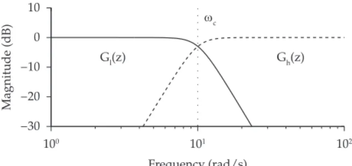
the same cut-off frequency ωc. For the experiments presented in the next section, first order digital filters with maximally planar response on the passband (Butterworth) and 10 Hz sampling rate were used. A typical frequency response of the CF filter can be seen in Figure 3.
The first filter significantly attenuates the high frequency accelerations of the first estimate (gravity projection and magnetic yaw orientation). The second filter suppresses the low frequency errors of the second estimate (due to bias and others uncertainties in the integration step of the gyros data). The filtering process is performed by a convolution in the time domain, as shown in Equations 12, 13 and 14. Finally, the two signals are summed in time, generating the final esti-mate of pitch, roll and yaw angles.
l a h g
= G *
G *
,
φ
φ +
φ
(12)l a h g
= G *
G *
,
θ
θ +
θ
(13)l m h g
= G *
G *
.
ψ
ψ +
ψ
(14)In general, ωc has a constant value, defined before the filtering process and used directly in the design of the filter. Its value can be different for each variable being filtered, and it is chosen based on the analysis of the frequency spectrum of each signal. It also depends on the sampling time of each sensor.
Here, we propose an adaptive filter in which we allow the filter project for each process iteration. So, we can change the cut-off frequency ωc in order to give more or less weight to
the high and low frequency signals.
In the first step, we choose the initial values for the cut-off frequency as we did for the non-adaptive case, by analyzing the frequency spectrum of “signal” of each angle. These values are defined as kφ, kθ and kψ for the CF of the roll, pitch and yaw angles respectively, and they are considered the ideal values for a non-accelerated robot with small roll and pitch angles.
Next, we consider the problem of calculating the adaptive
ωc for the case of the angles generated by accelerometers. As
pointed out before, the estimates of φ and θ are valid only if the vehicles is in inertial navigation. In this case,||a→||is equivalent to g0, and all assumptions made are correct. Unfortunately, when the robot navigates through irregular terrains, the above assumption is no longer true, and the
angular estimation may fail. So, we need to reduce the cut-off frequency of the CF in order to give less weight to the acceler-ometers and more weight for the gyros integration.
The Equations 15 and 16 show how this weighting is made. An exponential function was used because of the need to rapidly reduce the ωc when the measured acceleration
vector differs from the gravity vector.
|g0 a |
c
= k e
,
− − φ
φ
ω
(15)|g0 a |
c
= k e
.
− − θ
θ
ω
(16)We recall that the compass readings has a notable limi-tation, in that the heading values are more reliable when φ and θ angles of the robot (and consequently, the compass) are close to zero. So, we decide to use the simple solution of estimating the ideal value kψ as the maximum absolute value
of the angle between these two, as shown in Equation 17.
max(| |,| |)
c
= k e
.
ψ − φ θ
ψ
ω
(17)In the end, we have the orientation vector described as:
= [
].
Φ
φ θ ψ
In the next section, we extend this approach in order to estimate the robot’s position in the three-dimensional space. We use the same principles of the Adaptive CF to obtain a more reliable fusion between GPS and robot’s odometry.
3.3. Complementary filter for position estimation
In this section, we describe the second part of the meth-odology. A second CF is designed to combine the position estimates given by the robot’s odometry sensors and by the GPS sensor, producing a more reliable and more accurate final estimate of the robot’s localization on the six-dimen-sional configuration space.
3.3.1. Position estimation based on GPS measures
On the first stage of this second part, a GPS signal receiver fixed to the robot’s body was used to obtain an estimate of its global positioning. Usually, this estimate is given as a func-tion of the latitude, longitude and altitude of the receiver with respect to the Earth’s surface.
In this work, however, it is not necessary to know the robot’s position relative to the terrestrial inertial reference, since the displacements will be very small compared to the Earth’s radius. Hence, it is possible to assume that the Earth is approximately planar throughout the robot’s navigation space. A coordinate transformation from latitude, longi-tude and altilongi-tude of the GPS to the differential manifold of the Euclidian tridimensional space coincident with the NED frame is performed, and the GPS output may be considered as the xg, yg and zg signals.
As we will show at the end of this section, it will also be desirable to know the number of satellites Nsat seen by the GPS receiver. It will be used to adjust the cut-off frequency
100 101 102
−30 −20 −10 0 10
Frequency (rad/s)
Magnitude (dB)
ωc
Gl(z) Gh(z)
25 Adaptive complementary filtering algorithm for mobile robot localization
of the second Adaptive CF to reduce the confidence in this sensor whenever the number of satellites is reduced.
An interesting feature of using the CF technique is that the GPS signal, just as it happens with all sensors, contains noise and other variations. In the specific case of GPSs, one such effect which potentially has a large impact on localiza-tion is known as random walk. This effect is caused by high frequency variations which corrupt the satellite signals when the GPS receiver has either stopped or is moving slowly. This, and other similar undesirable effects, can be effectively reduced by filtering out the signal with a low pass filter.
3.3.2. Position estimation based on attitude and
odometry
Once the robot’s attitude in the tridimensional space is known, the next step consists on estimating the robot’s position. One simple solution is to integrate the kinematic differential equation (Equation 18) which describes the robot’s movement in space.
o
o o
o
x
cos cos
y
= v
sin
cos
,
z
sin
ψ
θ
ψ
θ
θ
(18)
where v0 is the measured velocity given by the robot’s
odometry sensor over time, and ψ and θ are the angles that
compose Φ→, estimated on the first part of our methodology.
The integration of this equation generates the x0, y0 and z0 signals relative to the robot’s odometry.
Just as discussed in the previous part, the estimation of a signal by numerical integration generates a measurement that is not reliable due to bias and other sensor noises from sensors. The integration process tends to amplify lower frequency signals of the variable, producing drift over time. Thus, in a complementary way to the GPS signal, the posi-tion estimates by odometry may be considered to be more reliable at higher frequencies. The two data streams are then combined using a second CF.
We also consider the fact that the GPS receiver is more affected by noise (such as Random Walk) when it moves with low (or null) velocity. This information will also be used to calculate the adaptive cut-off frequency in order to reduce the confidence on the GPS signal.
3.3.3. Position data fusion
Just as in the first part of the methodology, two different estimates were generated for each one of the variables that we wish to obtain, which present reliable information over different frequency ranges and, therefore, the fusion of these data should be factored in.
For that reason, the Adaptive CF technique was used:
two filters Gl and Gh with cut-off frequency ωc were designed
(whose value is not necessarily the same as the previous one). Equations 19, 20 and 21 show the calculation of the final values for the robot’s position.
l g h o
x = G * x
+
G * x ,
(19)l g h o
y = G * y
+
G * y ,
(20)l g h o
z = G * z
+
G * z .
(21)Again, we begin the filters project by choosing an initial
value kp which will be used as the ideal cut-off frequency for
all three variable position. In this step we use the same value
of ωc for the CF of x, y and z, as shown in Equation 22.
v N
y
x z o sat
c
=
c=
c= min(
c,
c),
ω
ω
ω
ω
ω
(22)where v0 Nsat
c
and
cω
ω
are calculated considering thefollo-wing constraints.
As mentioned before, the GPS uncertainty increases under low velocities and with a small number of satellites being registered by the receptor. We chose to treat these two effects separately, and take the minimum cut-off frequency between these two constraints.
For the velocity, we use the v0 parameters, provided by the
robot’s odometry sensor. Equation 23 presents the calculation
of the cut-off frequency, where vmax represents the maximum
translational speed achievable by the mobile robot.
vo v v
vo o max
c
= k
p1 e
.
− −
ω
−
(23)
A similar approach is used in Equation 24 to deal with the number of satellites information. Again, we use the expo-nential function in order to converge rapidly to low cut-off frequencies when these constraints are unfavorable. Here, the difference is that we have a minimum number of satel-lites for which this equation is valid, due to the GPS process calculation.
Nsat Nsat Nmax
Nsat p sat
c
k 1 e , if N > 3
=
0 elsewhere.
− −
−
ω
(24)
Finally, the vector that represents the robot’s position on the configuration space is given by
X = x y z .
(25)Along with the orientation vector, this vector is used to
compose the pose vector P→ at the end of each iteration of the
algorithm. Next, we compare the computational complexity of the algorithm that uses the Adaptive CF, in comparison with the most commons techniques used to make data fusion for robot navigation.
3.4. Computational complexity analysis
considering the use of this technique for robot localization in the three-dimensional space.
Gaussian Filters, such as Kalman Filter and its deri-vations (KF, EKF, UKF), are very commonly used in data fusion. The most expensive steps of Kalman Filters are the matrix operations (multiplication, inversion). The asymp-totically fastest algorithm known for matrix multiplication is
the Coppersmith-Winograd algorithm2, with complexity of
O(d2,376), where d represents the size of the square matrix. In
the specific case of Kalman Filters, this size is defined by the
number of state variables estimated14. Here we consider six
variables (three positions and three angles).
It is known that the computational cost of the Particle Filter technique depends on the number of particles m that we desire to use. The larger the number of particles, the greater the accuracy of the localization of the robot. According to
Thrun14, the computational complexity of this method is
given by O(m log m) The main problem with this is that the number of particles grows exponentially with the number of states d, which in practice is intractable for three-dimensional space.
The Adaptive CF technique is based on digital filtering theory. The Butterworth filter algorithm has a complexity that is proportional to the order n of the filter, or in other words, it is given by O(n). The proposed methodology uses a filter to
estimate each of the variables of the state vector (P→). It leads
to a complexity of O(nd), where d represents the number of variables of the state vector. In the experimental section we will show that first order filters (n = 1) are sufficient to build the CF. Therefore, our methodology has a linear complexity. It is less than half of the complexity of frequently used tech-niques such as UKF.
4. Experiments
The experiments were performed using real data acquired by a mobile robot while traversing an outdoor environment. During the robot’s navigation process, it collected and saved all sensor data, which were used as input to the simulation program.
The robot used was a Pioneer P3-AT model designed for outdoor applications. The P3-AT has a good load capacity, and data collection is performed by a laptop mounted on it, which is also responsible for sending commands to the robot. Figure 4 shows the arrangement of sensors on the robot.
In order to compute the attitude and position of the robot, the information provided by an IMU, a GPS, a digital compass, and the robot’s odometry sensor were used. The IMU used was the Crista by Cloud Cap Technologies, composed of three mutually orthogonal gyroscopes and three orthogonal accelerometers. A Garmin 18x-5Hz GPS was also used. It provides the absolute values of geographic position of the robot around the world and the number of satellites seen at every moment. The position information was used in terms of the Easting and Northing coordinates (form the coordinate system Universal Transverse Mercator, also called UTM), that are given in meters. Our set of sensors is completed by a KVH
C-100 Digital Compass, that is responsible for providing absolute values for the orientation of the robot according to the Earth’s magnetic north. It is composed by two magne-tometers disposed ortogonally in a planar form, and their values can be read directly from a serial interface.
Both IMU and compass present inside filters which are configured to remove noise from its signals. These filters were switch off because they affect the frequency response
of the measured variables, and produce great influence on
the final result.
As we mentioned before, in order to simplify the calcula-tions, it is assumed that the IMU is mounted exactly at the robot’s center of gravity, which in practice may not be neces-sarily true. Since the difference is very small and the speed of the robot is small, the setup is suitable for our approach. Hence, it is assumed that the robot and the IMU reference frames are coincident.
Three experiments were planned and carried out using the aforementioned setup, and they are describe next.
4.1. Experiment 1
In this first experiment the robot performed a path composed mainly of straight lines, and well defined curves (approximately 90°). The main objectives were to verify the accuracy of the robot’s localization, and to verify the possi-bility of correcting odometric errors by incorporating GPS data.
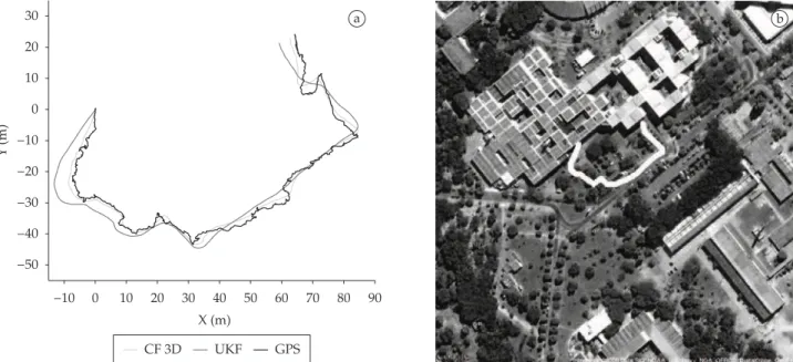
Figure 5a shows a comparison between three paths: the first one was performed by the robot based on the raw GPS data; the second, computed using our methodology, and the third path estimated by an UKF7, 14. As show in the figure, the raw GPS data is very noisy and clearly provides very low accuracy if used directly. The values obtained using our methodology, however, provided a smoother path closer to the one actually executed by the robot. It is interesting to note that the result was very similar to the one obtained by more complex techniques such as UKF.
Compass
IMU
Laptop
GPS
Odometry
27 Adaptive complementary filtering algorithm for mobile robot localization
The use of the GPS made it possible to correct the velocity errors obtained from odometric measurements. Another benefit of using GPS data is the possibility to obtaining the robot’s global localization. A great problem in experiments executed in outdoor environments is to get a ground-truth to compare the results. In order to verify the quality of the results, two different approaches were taken, one to vali-date the localization and another to check the orientation values.
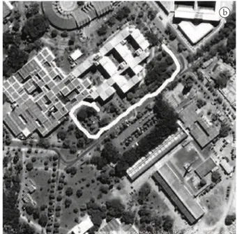
In order to verify how close the calculated localization is from the actual executed path, the calculated value was
drawn on a satellite image using an API4. Once the real path
is known, it is possible to validate that the calculated value corresponds to the real path. Figure 5b shows the path calcu-lated over an image of the region where the experiments were performed.
The orientation angles were validated by a comparison between two videos. One video corresponds to the executed moviments made by the robot, and that were recorded during the experiment. The second video was a 3D animation devel-oped based on the calculated values. It was then possible to conclude that the calculated values for the orientation angles corresponded to the effectively angles obtained by the robot during the execution of the experiment.
As observed in Figure 6, the data still contais a small amount of noise, however, the results were adequate for our purposes, and it represents the actual displacement performed by the robot. Analyzing the standard deviation of
the data we have σφ=2.4°,σθ=2.2°, while using the UKF the
standard deviations are σφ=1.8°,σθ=1.9°. We chose to not
calculate σψ, since the mean is not a good representation of
the values obtained.
Figure 5. Reconstruction of the path done by the robot on Experiment 1.
−40 −20 0 20 40 60 80 100 120 140
−60 −40 −20 0 20 40 60 80 100
X (m)
Y
(m)
CF 3D UKF GPS
a b
0 100 200 300 400 500 600 700 800
−15 −10 −5 0 5 10 15 20
Time (s)
Pitch (degr
ees)
0 100 200 300 400 500 600 700 800
−20 −15 −10 −5 0 5 10 15
Time (s)
Roll (degr
ees)
0 100 200 300 400 500 600 700 800
−300 −200 −100 0 100 200
Time (s)
Y
aw (degr
ees)
CF 3D UKF
a
b
c
The angle φ (Figure 6a) showed small variations due to imperfections in the terrain and signal noise, but at the end of the experiment it is possible to observe larger variations
(≈–4°) when the robot starts to descend a ramp.
The values of θ have, for the most part, zero mean (flat
terrain) however, between t = 230 s e t = 270 s (Figure 6b), the variation of (≈–2°) occurred while it descended an inclined region of the terrain where the experiment was carried out. Three other relevant disturbances, also related to terrain inclination, can be observed in the graph.
The result of ψ can be verified directly, since during the path the robot took four sharp turns (90° curves) that can be clearly seen in Figure 6c, represented by four large steps.
The values of altitude returned from the GPS are fundamental for the computation of the variation in the Z axis. Unfortunately, this value shows a large variation, and as such it is not a good representation of the actual displacement of the robot.
Figure 7 shows a comparison among the altitude calcu-lated by our methodology, the altitude computed by integrating the kinematic equation z0(t) (Equation 18), and the altitude zg (t) obtained directly from the GPS. Small vari-ations on the Z axis can be clearly observed at time instants t ≈240 s, t ≈ 410 s and t ≈ 690 s. The difference between the values of the highest and the lowest points returned from the GPS is ≈25 m, a value which is not consistent with the actual movement performed by the robot, which is well represented by the information obtained from z0(t).
Thus, the computed values for the variation in altitude were not reliable, and further analysis should be performed for an adequate incorporation of altitude data provided by the GPS. For the moment, and with the technology that was available to us, the measurements provided by the GPS contains much uncertainty. As a matter of fact, a more precise altitude data is required in order to correct the Z using our methodology as well as others, such as UKF.
4.2. Experiment 2
The next experiment consisted on making the robot navigates through different types of surfaces, with the main objective of verify the quality of the adaptation of the filter during the estimation of the orientation angles.
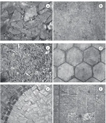
Figure 8 presents all types of surfaces visited the robot during navigation, where Figure 8a presents the most rugged terrain and represents the traversable limit of the used robot (since it moves with great difficulty in this type of terrain), and Figure 8b the less uneven terrain, the other surfaces have both rugged and planar parts.
The images in Figure 9 show the estimated trajectory for the navigation performed by the robot during the experi-ment.
Figure 10 shows the values of ωc for each different type of surface during Experiment 2. As it was expected, the rough the terrain the lower the cut-off frequency is, so, on terrain A the cut-off frequency is near zero.
It is possible to conclude that the terrain where the robot navigates directly affects the quality of the estimation, by adding noise to the values of the orientation angles, and consequently the localization.
4.3. Experiment 3
The main objective of Experiment 3 is to verify the quality of the calculation of ωc in the localization step, based on the number of satellites and the robot’s velocity.
It should be noted that during the execution of this exper-iment the robot never had fewer than seven satellites in sight, so, a complete loss of GPS signal has been simulated.
The images in Figure 11 show the estimated trajectory for the navigation performed by the robot during the experi-ment.
0 100 200 300 400 500 600 700 800
−15 −10 −5 0 5 10
Tempo (s)
Z (m)
z(t) (CF 3D) zo(t) (Odometry) zg(t) (GPS)
Figure 7. Altitude comparison for the complementary filtering using GPS.
a b
c d
e f
29 Adaptive complementary filtering algorithm for mobile robot localization
−10 0 10 20 30 40 50 60 70 80 90
−50 −40 −30 −20 −10 0 10 20 30
X (m)
Y
(m)
CF 3D UKF GPS
a b
Figure 9. Reconstruction of the path performed by the robot in Experiment 2.
Figure 10. Calculated ωc for the orientation angles during Experiment 2.
0 50 100 150 200 250 300 350 400
−0.05 0.00 0.05 0.10 0.15 0.20
Time (s)
0 50 100 150 200 250 300 350 400
Time (s)
0 50 100 150 200 250 300 350 400
Time (s)
Wc (
φ
)
A B D C D E F
−0.03 −0.02 −0.010.00 0.01 0.02 0.03 0.04 0.05 0.06 0.07
Wc (
θ
)
A B D C D E F
0.075 0.080 0.085 0.090 0.095 0.100 0.105
Wc (
ψ
)
A B D C D E F
Figure 12a shows how the speed of the robot varied throughout the trajectory. It is notable that lower speeds occur mainly during at curves, which some times are made in a turn-in-place manner due to the fact that the robot’s is of
the skid-steer type. Figure 12b show the ωc calculated based
on the velocity of the robot.
Figure 13 shows the results for the simulation of signal loss. It can be observed that a small error on the orientation generates large errors in the localization, where much of the error is related to the odometry. However, once the signal of the GPS becomes available again the path gets corrected.
5. Conclusions and Future Works
This work presented the use of the CF technique to estimate the full pose (localization and orientation) in the configuration space, for mobile robots navigating in outdoor environments on uneven terrain. The main advantage of the proposed technique is the significant reduction of the compu-tational complexity of the overall system, which enables increasing the sampling frequency of the signals with a consequent improvement in the accuracy of the estimates.
The results were satisfactory and very close to the values obtained with more complex techniques such as the UKF. This has been shown by plotting the actual path on satellite images, where the estimated path performed by using the proposed methodology have shown to be faithful to the actual path performed by the robot. We have also shown that height (change in Z axis) estimation was less accurate, mainly due to the large uncertainty on the altitude data provided by the GPS.
It was possible to obtain a good estimation of the
orienta-tion angles (φ,θ,ψ), but they still have a certain amount of
noise. The most accurate and reliable value was ψ, mainly
−150 −100 −50 0 50 100 −200
−150 −100 −50 0
X (m)
Y
(m)
CF 3D UKF GPS
a b
Figure 11. Reconstruction of the path performed by the robot in Experiment 3.
0 100 200 300 400 500 600 700 800
−0.1 0.0 0.1 0.2 0.3 0.4 0.5 0.6
Time (s)
0 100 200 300 400 500 600 700 800
Time (s)
V
elocity (m/s)
0.0 0.5 1.0 1.5 2.0× 10
–3
Wc
a
b
Figure 12. Comparison between the calculated ωc (b) and the robot
speed (a).
−150 −100 −50 0 50 100
−200 −150 −100 −50 0
X (m)
Y
(m)
CF 3D UKF GPS
Figure 13. Reconstruction of the path executed by the robot in Experiment 3 with GPS signal loss (simulated).
Although the experiments were conducted in an offline
way (post navigation processing), it was possible to observe that the method is very efficient, and amenable to be used in real time.
As future work, further experiments will be performed with larger vehicles, since it will make it possible to analyze the behavior of the system on greater scale experiments where the vehicle’s size is comparable to the path width restrictions.
Sensor processing continues to be an area of great rele-vance for robotics. Further investigation is demanded on sensors imperfections, such as bias in the IMU accelerometers
and gyros, in order to provide better methods to minimize even further their effects on the final estimations. Likewise, issues arising in other sensors such as magnetometers must be dealt with adequately.
31 Adaptive complementary filtering algorithm for mobile robot localization
Ackowledgements
The authors would like to thank Wolmar Pimenta for the support on the construction and integration of the mechanical system used in the experiments, and the financial support offered by the Fundação de Amparo a Pesquisa do Estado de Minas Gerais (FAPEMIG), the Conselho Nacional de Desenvolvimento Científico e Tecnológico (CNPq), and the Coordenação de Aperfeiçoamento de Pessoal de Nível Superior (CAPES).
References
1. Baerveldt AJ and Klang R. A low-cost and low-weight attitude estimation systemfor a autonomous helicopter. In: Proceedings of IEEE International Conference on Intelligent Engineering Systems; 1997; Budapest, Hungary. IEEE; 1997.
2. Coppersmith D and Winograd S. Matrix multiplicationvia
arithmetic progressions. In: Proceedings of the Nineteenth
Annual ACM Symposiumon Theory of Computing; 1987; New York. ACM; 1987. p. 1-6.
3. Euston M, Coote P, Mahony R, Kim J and Hamel T. A complementary filter for attitude estimation of a fixed-wing
uav. In: Proceedings of IEEE/RSJ International Conference on
Intelligent Robots and Systems; 2008; Nice, France. IEEE; 2008. p. 340-345.
4. Google Maps API. Google Code. [on the internet] 2008.
Available from: http://code.google.com/apis/maps/.
Access in: 29/07/2008.
5. Günthner W. Enhancing cognitive assistance systems with
inertial measurement units. New York: Springer; 2008.
6. Iscold P, Oliveira GRC, Neto AA, Pereira GAS and Torres LAB. Desenvolvimento de horizonte artificial para aviação
geral baseado em sensores MEMS. In: Anais do 5 Congresso
Brasileiro de Engenharia Inercial; 2007; Rio de Janeiro.
7. Jeffrey SJ and Uhlmann K. A new extension of the kalman filter to nonlinear systems. In: Proceedings of the 11International Symposium on Aerospace/Defense Sensing, Simulation and
Controls; 1997; Orlando, Florida. International Society for Optical Engineering; 1997.
8. Li Y, Wang J, Rizos C, Mumford P and Ding W. Low-cost tightly coupledgps/ins integration based on a nonlinear
kalman filtering design. In: Proceedings of the National
Technical Meeting of the Institute of Navigation; 2006, San Diego.
p. 958-966.
9. Liu B, Adams M and Ibañez-Guzmán J. Multi-aided inertial navigation for ground vehicles in outdoor uneven
environments. In: Proceedings of IEEE International Conference
on Robotics and Automation; 2005; Barcelona, Espanha. IEEE; 2005.
10. Mahony R and Hamel T. Advances in unmanned aerial vehicles:
state of the art and the road to autonomy, chapter robust nonlinear observers for attitude estimation of mini uavs. New York: Springer; 2007. p. 343-376.
11. Müller M, Surmann H, Pervölz K and May S. The accuracy
of 6D SLAM using the AIS 3D laser scanner. In: Proceedings of
International Conference on Multisensor Fusion and Integration for Intelligent Systems; 2006; Heidelberg, Germany.
12. Ojeda L and Borenstein J. Improved position estimation for mobile
robots on rough terrain using attitude information. Michigan: The University of Michigan; 2001. (Technical report)
13. Sukkarieh S, Nebot EM and Durrant-Whyte HF. A high integrity IMU/GPS navigation loop for autonomous land
vehicle applications. IEEE Transactions on Robotics and
Automation. 1999; 15(6):572-578.
14. Thrun S, Burgard W and Fox D. Probabilistic robotics: intelligent robotics and autonomous agents. Cambridge, MA: The MIT Press; 2005.
15. Thrun S, Diel M, and Hähnel D. Scan alignment and 3D
surface modeling with a helicopter platform. In: Proceedings
of the International Conference on Field and Service Robotics; 2003; Lake Yamanaka, Japan.
16. Walchko KJ and Mason PAC. Inertial Navigation. In: