Capital structure arbitrage : exploiting temporary mispricing between equity prices and CDS spreads using the CreditGrades model

Cap

ita

l Structure Arb

itrage – exp

lo

it

ing temporary

m

ispr

ic

ing between equ

ity pr

ices and CDS spreads

us

ing the Cred

itGrades mode

l

Sebast

ian Mart

in A

lber

D

issertat

ion wr

itten under the superv

is

ion of Professor

Nuno S

i

lva

D

issertat

ion subm

itted

in part

ia

l fu

lf

i

lment of requ

irements for

the MSc

in F

inance, at the Un

ivers

idade Cató

l

ica Portuguesa,

i

Abstract

This study implements a capital structure arbitrage strategy using the CreditGrades model and checks whether this is able to generate excess returns. Using a new methodology to identify mispricing triggers, and taking the EuroStoxx and a European Large Cap Bond Index as our benchmark portfolios, we find that our strategy is able to produce a significant alpha during the period between 2008 and 2015 (2.3% in annualized terms). We find however that our strategy is very dependent on trading opportunities, which tend to occur only when volatility rises above certain levels. In periods of prolonged low volatility, our strategy tends to generate weaker returns. As example, while in the period between 2008 and 2011 we obtain a significant annual alpha of 5.7%, in the period between 2012 and 2015 our alpha is only 0.25% and not statistically different from 0. Therefore, we can conclude our strategy is not able to deliver constant and significant abnormal returns in all periods.

Abstract Portuguese

A presente dissertação visa implementar uma estratégia assente em oportunidades de arbitragem relativas à estrutura de capital. Para tal, recorremos ao modelo CreditGrades e de seguida procuramos apurar se tal estratégia é capaz de gerar retornos incrementais. Sugerimos uma nova metodologia para identificar fatores que possam desviar os preços dos seus valores teoricamente justos e utilizamos o índice EuroStoxx e European Large Cap Bond Index como portfolios de referencia. Concluimos pelos resultados encontrados que a estratégia apresentada é capaz de gerar um alfa de 2.3% anualizado entre 2008 e 2015.Não obstante, reconhecemos que a estratégia que apresentamos depende de oportunidades de arbitragem existentes no mercado, as quais são mais comuns em períodos de aumento de volatilidade. Durante períodos de volatilidade contida, a estratégia que propomos apresenta resultados menos promissores. Entre 2008 e 2011 obtemos um alfa de 5.7%, enquanto que entre 2012 e 2015 registamos um valor inferior, de 0.25%, o qual é estatisticamente insignificante. Face a estes resultados, concluímos que a estratégia apresentada não é capaz de gerar retornos constantes e significativamente superiores em todos os períodos de tempo.

ii

Acknowledgements

Firstly I would like to thank my supervisor Nuno Silva, for the great support before and during the process of writing this thesis. Without him, this project would not have been possible. Secondly, I would like to thank my girlfriend Melanie Class for always supporting me, especially in the very stressful times. I would like to thank Duarte Stattmiller Stokes for the endless coding sessions at his place and his help regarding mathematical and matlab related questions. Furthermore I would like to thank all my friends at Católica Lisbon School of Business and Economics who made this program unforgettable. Last but certainly not least I would like to thank my parents without their support I wouldn’t be here where I am today.

iii

Contents

1. Introduction ... 1

2. Literature Review ... 4

2.1. Literature on Structural Models of corporate liabilities ... 4

2.2. Capital Structure Arbitrage... 9

3. The CreditGrades model... 15

4. Dataset ... 21 5. Trading Strategy ... 24 6. Results ... 28 7. Conclusion ... 36 8. References ... 38 9. Appendix ... 40

iv

Index of Figures

Figure 1: Relationship between Credit Spreads and Equity Prices 11

Figure 2: Description of CreditGrades model 17

Figure 3: Rating Breakdown 22

Figure 4: Trades Opened per Year 29

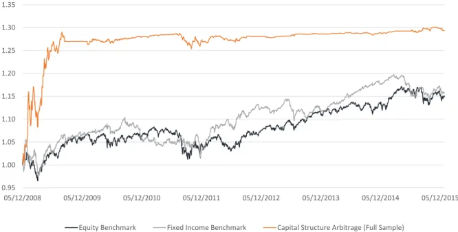
Figure 5: Wealth Evolution (scaled volatility) 31

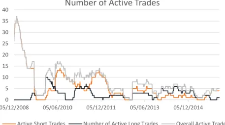
Figure 6: Number of Active Trades 33

Index of Tables

Table 1: Sector Allocation 21

Table 2: Descriptive Statistics of Correlation Measurements 22

Table 3: Descriptive Return Statistics 28

Table 4: Descriptive Return Statistics for Capital Structure Arbitrage vs. Benchmarks 30

Table 5: Quality of Trades 32

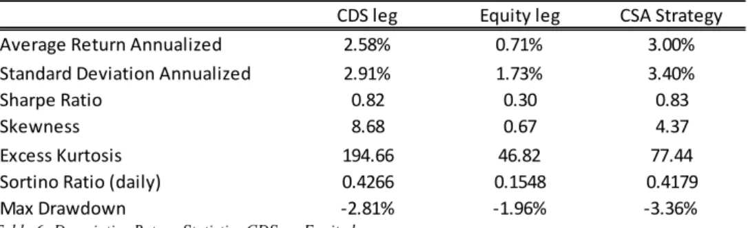
Table 6: Descriptive Return Statistics CDS vs. Equity Leg 32

1

1.

Introduction

The last years have been characterized by risk free interest rates near or even below zero in the case of shorter-term maturities. In such an environment, traditional strategies such as carry trades and riding the yield curve1 _{are no longer able to generate interesting returns, especially}

in the case of investment grade bonds. As result, several authors have pointed that this context is particularly favourable to the so-called search for yield, see Buch et al. (2011).

Possibly further contributing to this search for yield is the implementation of aggressive quantitative easing programs by all major central banks together with forward guidance in terms of future interest rates. These programs have contributed to create additional demand for sovereign and high rated corporate debt. As a result, private investors have been pushed to the high yield space or to very long maturities where one can still find some return at the cost of additional risk. This should be affecting both the shape of the yield curve and the market price of risk. The increasing demand in longer dated maturities is leading to a flatter yield curve, while the larger demand for high yield products may be further contributing to a reduction in the market price of risk, resulting in a compression in credit spreads. Ultimately, both developments lead to an increase in asset prices as pointed by Krishnamurthy and Vissing-Jorgensen (2011) and Joyce et al. (2012). This increase in asset prices comes however with substantial drawbacks in terms of risk. Though interest rates for several important benchmark rates have dropped already well into negative territory no one really knows whether they have already hit rock bottom or if they can go further negative. According to Coeuré Benoît (2015). we are very close or even at the lower boundary. This gives reason to see betting on further decreases in interest rates, especially through long term bonds, as a strategy having a long left skewed return distribution. In addition, a sudden reversal in the market price of risk and the following spike in yields could generate enormous losses for traditional fixed income investors. In this context, fixed income investors are currently thinking on implementing new trading strategies to deliver a return on investment compatible with their targets. In this article we examine if a capital structure arbitrage strategy is capable of producing stable and positive returns even in the current low interest rate environment. Capital structure arbitrage has been very popular with hedge funds as it should be able to deliver stable and constant returns in every

1 _{Carry trading consists of buying a bond and collecting its coupons until maturity, while riding the yield curve}

refers to a strategy where investors buy a long maturity bond and sell it after the price has increased due to lower short term rates.

2 phase of the market. The idea is to build a model for firm assets and conditional on this model find the price of several contingent claims, whose prices are available in the market, notably equity, credit-default swaps and option contracts. As debt and equity are seen as different derivatives of the same underlying, they must trade within a given range to each other and move together. Capital structural arbitrage strategies assume these differences are temporary and try to exploit them. In other words, the strategy consists of betting on the convergence between the observed prices and the ones given by the model. In the context of capital structure arbitrage, violations in this pricing relationship are seen as temporary and motivated by a different pace of price discovery. As further developed in section 2.2, in theory some markets (e.g. equity market) may incorporate new information faster than others (corporate bond markets) simply because they are more liquid, transparent, homogenous and have more participants. We may also have different investors in different asset classes that react differently on the same news. This may justify temporary violations in foreseen relations between contingent asset prices. Capital Structure Arbitrage simply intends to exploit this violation of the law of one price.

Underlying capital structure arbitrage are the so-called structural models of corporate liabilities, which find their roots on the seminal Black and Scholes (1973) and Merton (1974) papers. The literature on structural models of contingent liabilities is vast and has several purposes. The largest stream of the literature focuses on credit risk. Similar to traditional credit analysis, these models try to determine the probability of default and the appropriate credit spread of any obligor. However, while traditional credit analysis does it by using mostly balance sheet data, structural models focus on observed market prices. The fact that market prices should incorporate all available information should lead structural models to have, in theory, a superior performance over traditional credit analysis. After Leland (1994), structural models started also to be used to find the optimal capital structure of a firm. In the end of the nineties with the development of CDS markets and its boom phase during the first decade of the new century, the ability to trade debt increased drastically allowing the use of structural models also within the trading business. As one could now trade debt at given spreads, structural models could be used to judge if debt of any obligor was rich or cheap relatively to its equity price.

This master thesis implements a sophisticated trading strategy based on a structural model known as the CreditGrades model, see Finger et al. (2002). This is done based on a dataset consisting of daily CDS and equity prices for 67 non-financial European corporations covering the period between 2007 and 2015. Our main objective is to check if our strategy is able to produce constant and positive returns in all market phases.

3 This thesis is structured in the following way; Section 2 reviews the existing literature on structural models and their performance within capital structure arbitrage. Section 3 presents the CreditGrades model by Finger et al. (2002) and several posterior extensions to the original model. Section 4 reviews the dataset used in this thesis. Section 5 explains the trading strategy used. Section 6 discusses the empirical results of the structural model and the trading strategy. Finally, section 7 concludes.

4

2.

Literature Review

This section reviews the literature on structural models of corporate liabilities. First, the existing literature on structural models of contingent liabilities is reviewed. Due to their importance in the literature the papers by Merton (1974), Black and Cox (1976) and Zhou (2001) will be described in more detail. The CreditGrades model by Finger et al. (2002) is covered in section 3. The second part of this section reviews the literature regarding the theoretical fundaments behind capital structure arbitrage strategies as well as the implementation and the ability to generate excess returns of such strategies. As capital structure arbitrage is a complex undertaking involving different models, parameters and methods of calibration, all applied in different time spans, conclusions vary widely in literature.

2.1.

Literature on Structural Models of corporate

liabilities

At the foundation of structural models of corporate liabilities lies the model developed by Merton (1974). In this model it is assumed that a given corporation has only one single zero coupon bond outstanding. When the bond matures the firm is assumed to be liquidated. If assets are worth more than liabilities debtholders are paid fully and equity holders receive the residual. If they are worth less, the firm is said to default. In this case debtholders take all assets from the firm to compensate for their loss. Equity holders receive 0. Under this setting, the value of the equity can be modelled in the same way as the value of a European call. Similarly the debtholder position is equivalent to holding a risk free debt security and shorting a put option on the firm value. Assuming a flat term structure of interest rates, a Modigliani – Miller set – up, perfect markets and a firm value, which can be described as in equation (1), one can calculate the prices for debt and equity as shown in equations (3) and (4).

𝑑𝐴 = (𝛼𝐴 − 𝐶)𝑑𝑡 + 𝜎𝐴𝑑𝑧

where A denotes the value of the assets/firm, 𝛼 denotes the instantaneous growth rate of the assets, C denotes cash pay-outs such as dividends and z is a standard Wiener process. r expresses the risk free rate, 𝜏 the time to maturity of the zero coupon bond, B the face value of this zero coupon bond, 𝐸(𝐴, 𝜏) the value of the equity and 𝐷(𝐴, 𝜏) the value of the debt.

5

𝐷[𝐴, 𝜏] = 𝐵𝑒

{Φ[ℎ

(𝑑, 𝜎

𝜏] +

Φ[ℎ

(𝑑, 𝜎

_𝜏]}

The value of the firm is then given by

𝐴 = 𝐸(𝐴, 𝜏) + 𝐷(𝐴, 𝜏)

The spread of a bond can be easily computed from its bond price just rearranging equation (4).

𝐷[𝐴, 𝜏] = exp[−𝑦(𝜏)𝜏] 𝐵

Solving for y and taking out the risk free rate one obtains the model spread

𝑦(𝜏) − 𝑟 =

𝜏

log {Φ[ℎ

(𝑑, 𝜎

2

_{𝜏)] +}

𝑑

Φ[ℎ

(𝑑, 𝜎

2

_𝜏)]}

Unfortunately, empirical studies have shown that Merton model does not comply with real world observations. Especially, its inability to generate short-term default probabilities, and therefore credit spreads, which are compliant with empirical findings, prohibits practitioners from using the Merton model. The root of this problem lies in the assumption of the geometric Brownian motion. The variance of the firm value is, as shown in Merton (1974), a convex function of time, which results in a low variance for short maturities. For companies whose value is well above the default point (investment grade) this produces default probabilities close to zero as 𝜏 approaches 0. For companies that are close or even beneath the default point (high yield), default is virtually certain and spreads thus explode.

6 One practical way to work around the problem of low short term spreads was undertaken by Moody’s KMV.2 _{In their model, the idea is to first calculate a measure, which they called}

distance to default, that resembles how far the market value of assets is from a certain default point. Their measure can be computed simply as

𝐷𝐷 =

𝜎𝐴 (6)

Where 𝐴0 denotes the value of the assets in time 0, X denotes the default point and 𝜎𝐴

denotes the asset volatility. From this equation (6) one can easily observe that the distance to default is basically a count of standard deviations from the asset value until the default point. Using the default point one can easily calculate the probability of default:

𝑃𝐷 = 𝜙[−𝐷𝐷]

At this point, instead of evaluating the distance to default on the Normal distribution, Moody’s extensive database is used to map the calculated distances to defaults to empirical default probabilities. For example, using the basic Black & Scholes Merton set – up a distance to default of 4 would give a default probability of 0,003%. Using Moody’s KMV mapping procedure would give one a default probability of 0.4%, see Sun et al. (2012). Unlike other models, the aim of Moody’s KMV model is not to calculate the value of corporate debt but to quantify the default probabilities of a given debtor. While Moody’s KMV model produces higher default probabilities for short-term maturity investment grade bonds, it is academically speaking not coherent as it mingles normally distributed default distances with empirical default probabilities.

One of the largest issues in the Black Scholes set-up and therefore the Merton model is the assumption of normally distributed returns. There are very few all-equity firms outstanding. Notwithstanding this, there is enough empirical evidence that market returns tend to be leptokurtic meaning that they have a higher peak around its mean and a higher kurtosis (heavy tails) than the normal distribution. In addition, they tend to have a left skew. With their proprietary database, Moody’s is able to circumvent also this problem.

Other crucial assumption in Merton’s model is the idea that firms have only one zero coupon bond outstanding and that the firm is simply liquidated when this bond matures. As pointed by Black and Cox (1976), in the real world, firms issue several bonds with different

2 _{Moody’s KMV model has had several improvements. According to Sun et al. (2012), the model currently used}

7 maturities. In addition, bonds frequently have associated covenants in order to protect bondholders. Notice that modelling equity as a plain vanilla European call on the firm´s assets, Merton’s model comprises some perverse incentives to shareholders. As classic option’s pricing theory teaches, the value of any long position in options is a monotonically increasing function of volatility (positive Vega). The consequence of this is that equity holders just have to increase asset return volatility (i.e. take further risk) to increase the value of their claim. This is especially relevant whenever a firm is in financial trouble. In this case, management and equity holders might take irrational risks in order to attempt a kind of Hail Mary pass to safe their own positions. This phenomenon is known in the literature as gambling for resurrection. Debt holders usually have two preferred methodologies to prohibit management and equity holders from gambling for resurrection. One possibility is to introduce some kind of covenants in the debt contracts. Another way is lending money only for short periods. Whenever equity holders actions’ are perceived as too risky, debt holders simply “pull the plug” and not roll over their debt. Here the roll over dates act like check points, for debt holders to assess conditions again.

In order to solve this issue, Black and Cox (1976) propose the use of first passage time models. The model has the same assumptions about perfect markets as the Merton model. However, it models the equity of a firm as a down and out call option. Once the value of the firm falls below a specific threshold, the equity becomes worthless. Differently from Merton (1974) default can happen at any point in time and not just at debt’s maturity. As a result, shareholders position is no more monotonic on volatility meaning that shareholders incentives to gamble are now much lower.

The introduction of the barrier has also impact in terms of debt holders expected loss. Notice that this barrier establishes a lower boundary for the value of debt holders recovery. In absence of bankruptcy costs, the value of debt is a monotonically increasing function of this barrier. In the case where there are no default costs and the barrier is assumed to equal firm’s liabilities, debt holders expected loss is simply 0. In contrast, equity value is simply a monotonically decreasing function of this barrier. Without this mechanism, the value of firm could literally fall to zero without the debt holders being able to intervene.

Another crucial assumption in the Merton (1974) model is the idea that interest rates are constant. In an important paper, Longstaff and Schwartz (1995) propose a model where, in addition to a constant barrier, interest rates are considered to be stochastic according to the Vasicek model. Since Merton (1974) original papers there have been different approaches to

8 relax the assumption of a constant risk free rate (see for example Ramaswamy, Sundaresan (1986) and Maloney (1992)). Longstaff and Schwartz (1995) were, however, the first ones to find a closed form solution for a first passage in time model, incorporating dynamic interest rates. In addition, this model allows for complex capital structures and deviations from the absolute priority rule. The latter states that senior debt holders have to be repaid in full before junior debt and then equity holders can be repaid. In reality, however, the absolute priority rule hardly holds as for a restructuring all debt and equity holders have to approve. [Fabozzi (2002)] The use of stochastic interest rates is very important in pricing bonds, as the risk free rate is part of the discount factor for the principal and interest cash flows. However, in the case of CDS contracts the risk free rate enters the calculation mainly to discount the coupon payments and the CDS compensation in case of default.. These cash flows are rather small compared to the interest and principle payments of a bond. For this reason, the discount rate affects CDS prices to a lesser extent than it affects bond prices. In addition, as there is only a slightly negative empirical relationship between interest rates and credit spreads, one can assume interest rates are not an integral determinant of default probabilities (see Longstaff, Schwartz (1995) and Joon et al. (1993)). According to Lando (2004), if and only if the risk free rate is very volatile it has significant effect on CDS prices and thus the assumption of constant risk free rate is not problematic in most cases.

Unfortunately, both Black and Cox (1976) and Longstaff and Schwartz (1995) models fail to generate short-term spreads that are compliant with empirical findings. As previously referred, Moody’s KMV model found a practical way to solve this issue. As also referred, while their approach is very simple and effective, it is theoretically not correct. Nevertheless, other methods to achieve non-normal distributed default probabilities which are theoretical more consistent have been developed over the recent years. The most popular assume that assets follow some type of jump diffusion process. This is the case of Zhou (2001), He et al. (2011) and Ozeki et al. (2011). Escobar et al. (2012) assume that asset volatility is not constant3_{. Both}

cases lead to non-normal distributions. When jumps are introduced, the default becomes an unpredictable mathematical event, meaning that no one knows if the firm may default exactly in the next instant in time. This is in deep contrast with diffusion models for which default is said to be a predictable event. In the case of Zhou (2011), the dynamics of a firm asset value are described by the following equation (8):

3 _{Stochastic volatility models are able to generate tails. Nevertheless, as time to maturity reaches 0 the spread}

9

𝑑𝐴𝑡

𝐴𝑡

= (𝜇 − 𝜆𝑣)𝑑𝑡 + 𝜎𝑑𝑍

+ (Π − 1)𝑑𝑌

where

𝜇 denotes the expected return on the firm’s assets 𝑣, 𝜆 𝑎𝑛𝑑 𝜎 denote positive constants

𝑍₁ is a standard Brownian motion

dY is Poisson process with an intensity parameter 𝜆

𝛱 is the jump amplitude which must fulfil 𝛱 > 0 and has the expected value v+1

While the normal diffusion process resembles the normal “noise” around a firm’s value the jump process models sudden and large moves in the firm’s value. The latter can be due to public knowledge of new important information about the firm, e.g. fines, takeover attempts and much more. The value of the firm moves randomly and can drop at any time beneath the specified threshold without being exactly equal to it. The probability of the firm suddenly defaulting will depend on the hazard jump rate and on the volatility of the jump process. Also notice that, similarly to Merton (1974), but different from Black and Cox (1976), the recovery rate received by debt holders is stochastic meaning that debt holders do not know how much they receive in case of default. Given the nature of the jump process, there is however no closed form solution for this problem. The bond has thus to be priced using a Monte Carlo simulation approach.

2.2.

Capital Structure Arbitrage

Structural models of corporate liabilities treat equity and debt as two different claims contingent on the same underlying: the market value of the firm assets. The market value of assets is however unobservable and the maximum we can do is to estimate it based on the prices of all other claims. Based on this, one can then re-estimate what should be the correct price for these claims. Whenever divergences from the theoretical prices occur, the law of one price is violated, conditional on the model used. Such divergences from equilibrium prices can occur for a number of different reasons. Three reasons are commonly referred in the literature. First, it is usually stated that investors specialized in different asset classes may have different opinions about what is going on. This leads to different dynamics in different asset classes. Secondly, equity markets are usually said to feature a faster price discovery process as they are

10 very liquid and transparent and therefore able to incorporate new information much faster than debt markets. Norden and Weber (2004) compare the speed of price discovery in equity, CDS and bond markets and conclude in favour of this theory. Considering daily and weekly lead – lag relationships for their sample from 2000 to 2002 they find stock markets returns lead CDS and bond spread changes. This lead – lag relationship for stock market returns and CDS spreads does depend on the credit quality of the underlying corporation. For low quality credit firms this relationship is stronger. Finally, another explanation usually referred is related with the procedures involving the different types of investments. For instance, the downgrading of any bond shall lead to a big sell-off, as institutional investors may not be allowed to hold high yield bonds. Equity investors however are not required to fulfil any regulation of this type.

Some authors such as Duarte et al. (2007) suggest however that following the wide spread use of CDS contracts, the fundamentals behind capital structure arbitrage have most likely decreased. As standardized CDS contracts are more liquid than the underlying bonds, debt markets are now able to process information faster and therefore reach the equilibrium price in a timely manner. Even though the two markets have probably became more interconnected, existing literature still gives reason to believe that capital structure arbitrage is still able to lead to unexplained excess returns, due to inefficiencies in either debt and/or equity markets.

In addition, new regulations in the US, Great Britain and the EU prohibiting banks of being active in proprietary trading, and thus making market making less profitable, is expected to contribute to a slower process of price discovery in bond markets. Compared with equity markets, corporate debt markets are very fragmented and shallow. This fragmentation makes the presence of dealers mandatory to provide liquidity. When dealers have less capacity to buy and sell bonds, diminishing liquidity in the market, bid – ask spreads tend to increase. In extreme cases, such as a sudden spike in yields, the market experiences a big selling pressure, but as there is only limited buying power by dealers this will push prices further down. On the other hand, whenever the better part of investors wants to buy but there are simply not enough bonds available at dealers, this shall increase prices. One can easily see this would lead to a higher volatility in bond markets. Since the higher volatility is caused by bond market specificities, the effect on equity markets should be minor. There are at least two favourable scenarios for arbitrageurs. If movements in bond spread cause similar movements in the CDS market, this environment would lead to a vast number of lucrative trading opportunities for

11 capital structure arbitrageurs. If however, the movements in the bond market do not affect the CDS market, this would generate opportunities for CDS – bond basis arbitrageurs.4

Structural models assume that equity and CDS spreads are related through some function that varies among models. All of them have in common the idea that whenever assets go up, equity value should go up and CDS spreads should go down by certain amounts (and vice-versa). These amounts differ however from model to model. Assuming that the asset value is the only stochastic variable in the model, this implies that equity and CDS spreads are negatively related. In order for capital structure arbitrage to work, and though there might be some temporary perturbations, we hope that the true data generating process is consistent with this. In addition, we hope that our model is able to approximate the true relationship between CDS spreads and equity. Correctly approximating the relationship between CDS spreads and equity prices is crucial in capital structure arbitrage as it is used to determine the appropriate hedge ratio. If the model employed is not a good approximation of the true data generating process, one will not only receive subpar trading triggers, but also the hedge ratio will be imprecisely estimated, leading to an underestimation of the risk level incurred.

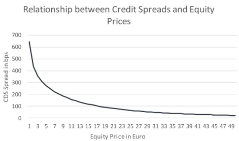
Figure 1: Relationship between CDS Spreads and Equity Prices in the CreditGrades model.. For this sensitivy analysis all other input parameters such as volatility, debt per share ratio, the risk free rate,time to maturity, recovery rates and the volatility of the default barier have been held constant.

As can be seen in Figure 1, our model does not imply a linear relationship between equity prices and CDS spreads. The first derivative of our function is always negative but it converges to 0 as equity increases. This makes sense as for high equity prices default

4 _{The CDS – Bond basis refers to the difference in spreads a bond and a CDS contract on the same obligor have.}

Theoretical the difference should be very small, only compensating interest rate risk in bonds. Otherwise it would be possible to construct a risk free asset yielding a different return than the risk free benchmark.

0 100 200 300 400 500 600 700 1 3 5 7 9 11 13 15 17 19 21 23 25 27 29 31 33 35 37 39 41 43 45 47 49 C DS Sp re a d i n b p s

Equity Price in Euro

Relationship between Credit Spreads and Equity Prices

12 probabilities are already close to zero and thus debt holders do not gain as much from a further increase.

Though structural models point to a clear negative relation equity value and CDS spreads, empirical evidence on this fact in capital structural arbitrage literature has been weak. Different authors suggest various correlation of debt and equity markets. For instance, Currie and Morris (2002) state that correlations between equities and debt of the same company are between 5% and 15%. One should be however very careful when we test whether equity markets and CDS markets are in fact related. The use of linear correlation measures as Pearson correlation might be misleading as the relation between equity and CDS spreads should be highly non-linear as structural models suggest. Rank correlation measures such as Spearman rho or Kendall’s tau should be more appropriate in these cases. Unfortunately, the authors do not state whether they calculated the Pearson correlation coefficient or a rank correlation coefficient.5 _{The low correlations could also be explained by the lead – lag relationship}

described by Norden and Weber (2004). For a more thorough examination, one could form portfolios using weekly or even monthly returns to minimize the effect of the lead – lag relationship on correlations6_.

Previous paragraphs discussed the foundations of capital structure arbitrage. This study will now revise the literature on its performance. As capital structure arbitrage is a complex undertaking involving different models, parameters and methods of calibration, all applied in different time spans, conclusions vary widely in literature.

Yu (2005) examines the risk – return properties of capital structure arbitrage using the CreditGrades model. Daily CDS spreads of 33 companies between 1997 and 2004 are analysed. The implemented trading strategy accounts for trading costs by using a bid – ask spread for CDS of 18%. The use of data from a period where the CDS market was not as liquid as it is today motivated Yu (2005) to use this high bid – ask spread. Yu (2005) concludes that capital structure arbitrage is able to generate significant excess returns, though he finds the strategy risky. This finding suggests the name capital structure arbitrage is misleading. Especially in the case where the trigger signalling that the market is being inconsistent is set at a low level, Yu (2005) finds a high standard deviation in holding returns and at times a negative mean of such

5 _{For our dataset the average Pearson correlation coefficient is -0,21 while the average rank correlation}

coefficient is -0,25. A detailed description of the dataset will follow in section 4.

6 _{In appendix H one finds the average rank correlation coefficient for daily, weekly and monthly changes in}

13 returns. 7 _{As stated in the paper, the high losses come mostly from shorting CDS contracts.}

Shorting CDS contracts is very risky as the non-linearities in the CDS-equity relation turn the hedge position (i.e. shorting stock) ineffective. One could simply not execute trades where one has to short CDS contracts. This would reduce considerably the number of possibilities to do capital structure arbitrage, though8_{. As an alternative, one can update the hedge ratio more}

frequently or simply over hedge such trades by shorting a larger amount of stock. Despite the riskiness of the strategy, Yu (2005) recognizes that capital structure arbitrage is very capable of producing very attractive returns. In its most promising set – up Yu (2005) is able to produce average monthly excess return of 10% and an annualized Shape ratio of 1.54. One should be however critical of Yu (2005) results as his data set is composed of only 33 obligors and his most promising set – up was obtained in an in – sample exercise.

Duarte et al. (2007) present a completely different picture. In their study, they compare different fixed income arbitrage strategies. Among these strategies, they implement a simple version of capital structure arbitrage using the CreditGrades model. They do it for 261 obligors covering the period between 2001 and 2004. A 5% bid – ask spread for CDS is assumed but equity specific trading costs are not considered. Duarte et al. (2007) approximate fees using the hedge fund standard 2% and 20% model in addition to the transactions costs10_{. Three of the six}

strategies published by Duarte et. al. (2007) have positive monthly excess returns that are significant at the 5% level. In addition, in contrast with Yu (2005), Duarte et al. (2007) conclude that all six capital structure arbitrage strategies have a positive skewness and excess kurtosis. Running regressions on common risk factors, their capital structure arbitrage strategy is able to produce positive alphas, before and after fees. However, after fees only the strategy with the highest trigger in the speculative bond universe produces an alpha of 0.680%, which is statistically significant at the 10% level. Obviously, there is a trade – off between the engagement in trades and the risk of the strategy. One could simply engage in any trade whenever the model detects a minor mispricing in the hope of future convergence. This could lead however to higher trading costs and more risk. Duarte et al. (2007) test different strategies with different entering triggers for speculative and investment grade obligors. Unfortunately, their numbers are not comparable with ours since we use a different calibration procedure.

7 _{The triggers are a measurement of the divergence between model and market spreads. For a larger trigger}

the divergence between both spreads needs to be larger in order to enter a trade.

8 _{See appendix E.}

10 _{Investors typically pay 2% of their assets as an annual fee. On top of that a 20% performance is usually}

14 Cserna and Imbierowicz (2008) find results similar to those from Duarte et al (2007). They find that for their sample period from 2002 to 2006 the CDS market was inefficient with capital structure arbitrage being able to generate positive excess returns. Their sample consisted out of 808 obligors, which is much larger than Yu (2005) and Duarte et al (2007). The standard 5% bid – ask spread for CDS was used. In addition, a 0.1% bid – ask spread for stocks was considered. Contrarily to previous papers that focused on the CreditGrades model, this study does a comparison between different structural models. In their study, the CreditGrades model was able to produce Sharpe ratio of 0.77 for the time period between 2002 and 2006 with a clear negative trend over the years. The Zhou (2001) and Leland and Toft (1996) models were however able to outperform the CreditGrades model both with a Sharpe ratio of 0.79. They also conclude that the efficiency of CDS markets has increased over the later period of their sample as excess returns have been decreasing. As most studies, Cserna and Imbierwociz (2008) find capital structure arbitrage is most lucrative for low credit quality firms.

A very recent study by Wojtowicz’s (2014) implements the CreditGrades model and using a sample covering the period between 2010 and 2012. He finds nearly 60% of the trades end in convergence with trading possibilities clustering in time, though.12 _{The mean holding}

return of this trades after transactions costs is 6.59% and the maximum loss registered by their strategy was substantially below 5%. Notice however that Wojtowicz’s (2014) considers a very short time frame. As the strategy implemented in this study is very similar to the one followed by Wojtowicz’s (2014), a closer examination of the methodology will follow in section 3.

15

3.

The CreditGrades model

As previously said, several approaches have been proposed in order to solve the fact that first generation structural models were unable to generate sufficiently high credit spreads for short-term investment grade bonds. We have already discussed two alternatives, notably, the practical oriented approach followed by Moody’s KMV, which relies on an extensive proprietary database, and the more theoretical consistent proposal of Zhou (2001), who considers that assets follow a jump-diffusion process. In this section, a third alternative is considered: the CreditGrades model.

The CreditGrades is a quantitative single-name credit risk model developed by RiskMetrics Group, Inc. together with Goldman Sachs, JPMorgan and Deutsche Bank. As pointed by Currie and Morris (2002) and Yu (2006), the CreditGrades model soon became the standard industry model for measuring credit spreads.. The technical details of this model are presented in Finger et al. (2002). While the authors were very well aware of the problems of diffusion processes in modelling short-term credit spreads, the CreditGrades model avoided the introduction of jumps. Instead, an uncertain default barrier is introduced. As discussed in this section, the introduction of uncertainty in the barrier turns default into an unpredictable event. This enables the model to produce higher short-term spreads even for investment grade bonds. The fact that the model still relies on the classic geometric Brownian motion allowed its authors to find a closed form solution for CDS spreads13_{. This is a great advantage in comparison to the}

more complex jump-diffusion models.

The CreditGrades model assumes that the firm value follows a geometric Brownian motion. Therefore, changes in the firm value follow equation (9):

𝑑𝐴_𝑡

𝐴_𝑡

= 𝜇

𝑑𝑡 + 𝜎𝑑𝑊

where W defines a standard Brownian motion, 𝜎 denotes the asset volatility and 𝜇𝐴 the asset

drift. It is assumed that the company issues continuously new debt at a pace equal to the risk free rate. This implies that under the risk neutral measure nominal debt has the same drift as the

13 _{The closed form solution in Finger et al (2002) only approximates the correct survival probability. The correct}

way to compute the survival probability is shown by equation 21 using the method proposed by Kiesel and Veraart (2008).

16 market value of assets. In relative terms, the drift of the assets to the default barrier (debt) is zero, and thus the leverage ratio is expected to remain constant in the risk neutral measure.

Using the CreditGrades model the default barrier (L), follows a lognormal distribution with expected value

𝐿̅

𝜆

.

𝐿𝐷 = 𝐿̅𝐷𝑒

where:

𝐿̅ = 𝐸(𝐿)

𝜆

_{= 𝑉𝑎𝑟 𝑙𝑜𝑔(𝐿)}

Z is said to be a standard normal random variable, which is independent of the Brownian

motion W. According to the Portfolio Management Data and Standard & Poor’s database 𝐿̅ should take the value of 0.5 and 𝜆 of 0.3 [Hu and Lawrence (2000)].14 _{D denotes the value of}

debt per share.

Please note for a higher 𝜆2 _{the default barrier may take larger values and therefore}

increases the risk of a default

14 _{For the financial sector 𝜆 should take a lower value due to specific government regulation. [Finger et al.}

17 Figure 2 Description of CreditGrades model, Source: Finger et al.( 2002)

In order to implement the CreditGrades model, one has to estimate various input parameters. Regarding D, which is the debt-per-share, the following steps should be pursued. First, one has to calculate the financial debt of any given firm, which is equal to:

𝐹𝑖𝑛𝑎𝑛𝑐𝑖𝑎𝑙 𝑑𝑒𝑏𝑡 = 𝑆ℎ𝑜𝑟𝑡 𝑡𝑒𝑟𝑚 𝑖𝑛𝑡𝑟𝑒𝑠𝑡 𝑏𝑒𝑎𝑟𝑖𝑛𝑔 𝑑𝑒𝑏𝑡 +

𝐿𝑜𝑛𝑔 𝑡𝑒𝑟𝑚 𝑖𝑛𝑡𝑒𝑟𝑒𝑠𝑡 𝑏𝑒𝑎𝑟𝑖𝑛𝑔 𝑑𝑒𝑏𝑡 + 0,5(𝑂𝑡ℎ𝑒𝑟 𝑠ℎ𝑜𝑟𝑡 𝑡𝑒𝑟𝑚 𝑙𝑖𝑎𝑏𝑖𝑙𝑖𝑡𝑒𝑠 +

𝑂𝑡ℎ𝑒𝑟 𝑙𝑜𝑛𝑔 𝑡𝑒𝑟𝑚 𝑙𝑖𝑎𝑏𝑖𝑙𝑖𝑡𝑖𝑒𝑠) (11)

where other liabilities refer to liabilities such as tax liabilities and pension liabilities.

In a second step, one has to adjust for minority debt. This is done subtracting Minority debt, which is nevertheless capped at 50% of the Financial Debt.

Debt = Financial debt – Minority debt (12) In a third step, one has to calculate the Number of shares. This is done by adding up the number of Common shares and the number of Preferred shares where

Common shares = Market cap / Stock price and

Preferred shares = Preferred equity / Stock price (13) Finally, Debt per share equals to

18 As with all diffusion processes, its path largely depends on its volatility. In opposition to the Black Scholes case, the underlying asset cannot be observed in the market, turning volatility estimation more difficult. Finding a good estimator for the asset volatility is key in implementing this model. One possibility proposed in Finger et al. (2002) is to use a 1000 day historic average of the equity volatility as an input factor for the asset volatility calculation. Following the application of Ito’s lemma, it is possible to show that asset and equity volatility are linked through financial leverage with the following equation (15):

𝜎

= 𝜎

𝑆 𝜕𝑆

𝜕𝐴

S denotes the stock price for a given firm and 𝜎𝑆 denotes the equity volatility.

Following equation (15) and assuming that A = S + LD, and thus the derivative of A with respect to S equals 1, we end up with the following relation between asset and equity volatility.

𝜎

= 𝜎

𝑆+𝐿𝐷 (16)

According to equation (16), equity volatility is rising giving a fall in stock prices and a constant asset volatility. This is in line with empirical findings that companies closer to default tend to show higher equity volatility. This relationship is commonly referred to as the leverage effect.

Now as all input parameters have been discussed one can compute the survival probability by the following equation (17). Based on Finger et al. (2002), the survival probability is given by

𝑃(𝑡) = 𝜙 (−

+

) − 𝑑 ∗ 𝜙 (−

+

)

𝑑 =

𝑒

𝐴

= (𝜎

)

𝑡 + 𝜆²

19 𝜎_𝑆∗ = 𝑟𝑒𝑓𝑒𝑟𝑒𝑛𝑐𝑒 𝑠𝑡𝑜𝑐𝑘 𝑣𝑜𝑙𝑎𝑡𝑖𝑙𝑖𝑡𝑦

D = debt per share

𝐿̅ = global debt recovery rate

𝜆 = percentage standard deviation of the default barrier

The survival probability function is then used to compute CDS spreads as followed:

𝑐

= 𝑟 (1 − 𝑅)

𝑃(0)−𝑃(𝑡)𝑒−𝑟𝑡_−𝑒𝑟𝜉_{(𝐺(𝑡+𝜉)−𝐺(𝜉))} (20)

where 𝜉 = 𝜆_𝜎22, and G is given by Rubinstein and Reiner (1991):

𝐺(𝑡) = 𝑑𝑧+0,5𝜙 (−log(𝑑) 𝜎√𝑡 − 𝑧𝜎√𝑡) + 𝑑 −𝑧+0,5_{𝜙 (−}log(𝑑) 𝜎√𝑡 + 𝑧𝜎√𝑡) 𝑧 = √1 4+ 2𝑟 𝜎2

R denotes the asset specific recovery rate while r denotes the risk free rate. In the CreditGrades

technical document R is set to 0.3. As R is used to estimate the recovery rate of unsecured debt is must be smaller than

𝐿̅

In 2008, Kiesel and Veraart (2008) pointed out that the formula for calculating the survival probability used by Finger et al. (2002) was wrong. They argue that it is only an approximation, which in cases of high leverage, can lead to substantially different survival probabilities and therefore CDS spreads.15 _{Kiesel and Veraart (2008) state that the correct}

equation (21) to calculate the survival probability is:

𝑃(𝜏) = Φ

(−

+

, −

+

;

) − dΦ

(

+

, −

−

; −

)

(21)

15 _{Kiesel and Veraart (2008) show that whenever the share-to-debt ratio is below 0.796, the}

20 Over the years there have been various extensions of the CreditGrades model. Stamicar and Finger (2006) proposed incorporating equity derivatives into the CreditGrades model in three different ways:

1. Estimating asset volatility by ATM options, but leaving all other input parameters as in the previous version.

2. Estimating asset volatility by ATM options and estimating leverage using CDS contracts.

3. Estimating asset volatility and leverage by using two different options.

The rationale behind their extension is obvious when one acknowledges that option implied volatilities are forward looking. Especially the 1000-day historical average used by Finger et al (2002) seems to be critical as it doesn’t respond quick enough to an increase in volatility following a deterioration in credit quality. Estimating leverage from market data can be useful for trading strategies when balance sheet data is not made available entirely or is not accurate enough, due to large holding of secured debt.

One alternative to the above-mentioned approaches is to use CDS implied volatilities as proposed by Wojtowicz (2014). Wojtowicz (2014) calculates the implied asset volatility using existing market CDS spreads. Then the model CDS spreads are computed by using a one-year average of the daily CDS implied volatility. This strategy guarantees that market and model prices are never too far from each other avoiding an abnormal number of trades for some issuers. In addition, under this approach the model is constantly recalibrated This contrasts with Yu (2005) where the model is calibrated once using a 10-day burn in period. In this article, the basic CreditGrades model is implemented with asset volatility being estimated as proposed by Wojtowicz (2014).

21

4.

Dataset

The data set used in this article consists of 67 non financial corporations from the Euro area. For these companies we have downloaded daily equity prices and CDS spreads from 14.12.2007 to 31.12.2015 from Thomson Reuters. The 5 year risk free interest rate, which is approximated by the ISDA fixed middle rate, was also taken for the same time period. The initial dataset used in this study was comprised of 97 corporations. Nevertheless, we have excluded companies, whose CDS contracts were not regarded as being liquid. In order to identify these companies we have checked for the first 250 days if there has been a consecutive period of 30 days where no trading activity has taken place. If this was the case, we excluded this company from our sample. Such a screening is important as for illiquid contracts, the assumption of being a price taker may not hold.

As shown in Table 1 our dataset comprises firms from a great number of economic sectors. ‘Consumer Discretionary’ and ‘Industrials’ are the sectors with the highest weight.

Table 1: Sector Breakdown of the examined company. Financial corporations were not considered, as estimating their appropriate debt per share ratio is not as straight forward as for non-financial corporations

In Figure 2, the current rating breakdown of the companies examined in this study can be observed. Investment Grade corporations correspond to 82.09% (55 companies) while companies within the high yield space total only 7.46% (5 companies). Not Rated companies account for 10.45% (7 companies) of the sample. Our sample is very concentrated in the Investment Grade space. This is partly the result of our filtering process, which resulted in a great number of non-investment grade firms being eliminated from our data set.

Sector # of companies percentage

Energy 4 6% Information Technology 2 4% Consumer Staples 6 9% Health Care 2 4% Consumer Discretionary 15 21% Materials 8 15% Telecommunication Services 4 7% Industrials 15 21% Utilities 11 12% Sum 67 100% Sector Allocation

22

Figure 3 Current rating breakdown (S&P Ratings) of all examined corporations

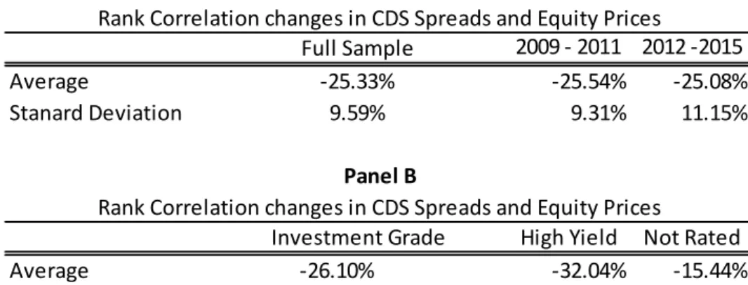
As mentioned in section 3, the existence of a significant level of correlation between CDS spreads and equity prices is crucial for capital structure arbitrage to be a successful strategy. In Table 2, one can find the rank correlation coefficient for the dataset.16 _{In panel A,}

one finds the rank correlation coefficient for three different sub periods. The first period ranges from 2007 to 2011 and includes the financial crisis and the European sovereign debt crisis. The second period, which comprises the years from 2012 to 2015, was marked by very low interest rates and the implementation of aggressive quantitative easing programs in the euro area. In panel B one finds correlations split by Investment Grade, High Yield and Not Rated obligors.

Table 2: Descriptive statistics of correlation between changes in equity prices and changes in CDS spreads

From Table 2 one can see that correlations between equity prices and CDS spreads are more significant than the figures referenced by Currie and Morris (2002) and Yu (2005), which

16 _{Only the rank correlation is presented in this study as the relationship between CDS spreads and equity prices}

is assumed to be non-linear. However, for the case of daily returns, we found the Pearson correlation to be quite close to the rank correlation coefficient.

2009 - 2011 2012 -2015

Average -25.54% -25.08%

Stanard Deviation 9.31% 11.15%

High Yield Not Rated

Average -26.10% -32.04% -15.44%

Investment Grade

Panel B

Rank Correlation changes in CDS Spreads and Equity Prices Full Sample

-25.33% 9.59%

Rank Correlation changes in CDS Spreads and Equity Prices

Panel A

Discriptive Statistics of Correlation Measurements 9.0% 6.0% 13.4% 20.9% 19.4% 13.4% 6.0% 1.5% 10.4% Rating Breakdown A+ A A- BBB+ BBB BBB- BB+ BB NR

23 tend to be close to 0,20 in absolute value. For our sample, correlations have appeared to be very stable over time. Unsurprisingly correlations for high yield corporations are more significant than for investment grade or not rated obligors. This is in line with the findings in previous studies pointing that equity and CDS markets tend to be more interconnected when firms are closer to default.

24

5.

Trading Strategy

The trading strategy implemented in this thesis is based on the CreditGrades model. Whenever there is a large enough divergence between market and model CDS spreads, it is assumed that there is some type of mispricing in either the CDS or the equity market. CDS spreads and/or equity prices should thus eventually converge to the ones estimated by our model. The market is considered not to be consistent with the model whenever one of the following occurs for a 5 year CDS contract:

𝑀𝑜𝑑𝑒𝑙 𝑆𝑝𝑟𝑒𝑎𝑑 > 𝑀𝑎𝑟𝑘𝑒𝑡 𝑆𝑝𝑟𝑒𝑎𝑑 + (𝑑̅̅̅ + 𝑎 ∗ 𝜎_{𝑐 𝑑}) 𝑀𝑜𝑑𝑒𝑙 𝑆𝑝𝑟𝑒𝑎𝑑 < 𝑀𝑎𝑟𝑘𝑒𝑡 𝑆𝑝𝑟𝑒𝑎𝑑 − (𝑑̅̅̅ + 𝑎 ∗ 𝜎_{𝑐 𝑑})

where 𝑑̅̅̅𝑐 denotes the moving average for the previous c days of the absolute difference

between the market and the model CDS spreads, 𝜎𝑑 is the standard deviation of the differences

over the specific period and, finally, 𝑎 and c are parameters which have to be estimated. The parameters used in this study are 4 for 𝑎 and 20 days for c. This set of parameters was found by optimizing the Sharpe Ratio across the whole sample17_{. This procedure presents two advantages}

over the static approaches normally used in existing literature. First, by using a moving average and a standard deviation measure, we are able to customize trading signals to the time series properties of each company. In contrast, other procedures described in the literature, which use the same parameters for all companies, require market spreads to deviate a lot more from model spreads in absolute terms in the case of riskier firms. This creates a kind of bias with trading signals tending to be more frequent than the optimal level in the case of safer firms. The opposite occurs in the case of riskier firms. Secondly, the thresholds used in most studies are static meaning that they do not change over time and thus are not able to adjust when the surrounding environment changes, e.g. a faster price discovery process in the debt market may lead to a reduction in the average difference between model and market CDS spreads. In contrast, our threshold values change through time.

Similar to Wojtowicz (2014) we assume that convergence has occurred whenever the model and the market spreads trade within a 1% interval. The fact that the probability of further convergence being in principle positively related with the divergence size indicates that there should be scope for capital structure arbitrageurs to optimize also on the exit threshold.

17 _{In appendix A we present a parameter sweep, which shows the Sharpe Ratio for 400 different combinations}

25 Nevertheless, the fact that we restrict the holding period to 180 days mitigates the impact of this.18

In order to implement our strategy, our sample of 67 companies was divided into 67 portfolios each of which consisting of one single company. In the beginning of the period, an equal amount of capital was assigned to each portfolio. As previously referred, under our strategy a trade is entered whenever the market and model CDS spreads are considered to be too far away from each other. Two cases may occur. We may have either a short position on the CDS market (short position on stocks) or a long position on the CDS market (long position on stocks). There are, however, some important issues one must take into account in the case of shorting CDS contracts. In particular, no one wants insurance from someone that is not trustworthy. The investor who buys the protection wants to be sure that the protection seller has enough funds to honour the contract in times of default. Whenever this is not assured, there might be reasons for a counterparty premium in the CDS contract, which may undermine our strategy. A credible risk management system is therefore particularly important whenever holding short positions on CDS contracts. This should involve measuring the credit value-at-risk of our portfolio at each moment in time. Alternatively, one could simply avoid entering into trades that involve shorting CDS contracts19_{. In this study, and though no effective risk}

management tool was considered, both short and long positions were considered. Nevertheless, the relationship between the notional of the CDS and the initial capital, which we called leverage, was restricted to 5, meaning that one could trade a CDS contract with a notional of 5 million Euros with initial capital of only 1 million euros. In addition, a stop loss mechanism has been implemented. The latter implies that, whenever the value of the security portfolio has dropped by 50% or more of its maximal value, we are forced to liquidate the position.

In order to evaluate our strategy, we need to estimate the value of our portfolio at each moment in time. This correspond to the sum of all outstanding CDS contract values, equity investments and of our current cash position. It is trivial to estimate the daily returns of the equity leg of our strategy. In order to construct the daily returns of the CDS portfolio, as there is no liquid secondary market for such contracts in all maturities, one needs however to calculate the daily theoretical values of these contracts. A newly issued CDS contract is worth 0 at its issuance as the initial spread ensures both legs, the one paid by the buyer (coupon leg) and the

18 _{Notice, however, that whenever a firm is still within the limits of our entrance thresholds, and though we close}

our position after 180 days, a new position is created in the next day. So, this rule is only effective for the cases where some convergence has occurred but not enough to reach our exit threshold.

19 _{In the appendix, one can find return statistics on a strategy where shorting CDS is prohibited. Results are very}

26 one received by the buyer (default leg) are exactly worth the same. Over time markets appraisal on global and firms conditions change and the negotiated spread is no longer ensuring an equilibrium price of 0. For instance, when default probabilities rise the CDS contract has a positive value to the protection buyer (and a negative one of to the seller). However, when default probabilities decrease, the CDS contract has a negative value to the buyer and a positive value to the seller. Computing the value of an existing CDS contract is important; as we have to take into account the cash flow of selling such a contract after convergence has occurred. In this study, we do it following Yu (2005), who states that a long position in a CDS contract is worth

𝑉(𝑡, 𝑇) = (𝑐(𝑡, 𝑇) − 𝑐(0, 𝑇)) ∫ 𝑃(𝑡, 𝑠)𝑞

(𝑠)𝑑𝑠

𝑇

𝑡 (22)

where c(t,T) is the current spread of an existing CDS contract, c(0,T) is the spread of the CDS contract when it was negotiated first and 𝑞𝑡denotes the survival probability from time t until

maturity in T. P(t,s) denotes the price of a discount bond. The survival probability is computed using the CreditGrades model. Notice that the valuation of the CDS contract depends mostly on the spread change and only to a lesser extent on the survival probability, which is model based. Using this equation to value our CDS position one needs secondary market quotes on any given day for a CDS contract with the specific residual maturity. As this data is not available Yu (2005) approximates c(t,T) by c(t,T+t), where the latter corresponds to the CDS spread on a newly issued CDS contract with the same maturity as the initial CDS contract. One alternative to this would be simply to do some type of interpolation based on the observed CDS curve. Nonetheless, Yu (2005) argues that the holding period t is usually very small in relation to the maturity and thus this approximation should lead to good results. Since we are using only 5 year contracts, which are the most liquid, and we do not allow holding periods above 360 days we follow the argumentation and methodology of Yu (2005).

As our strategy is, theoretically, an arbitrage strategy we do not place outright directional bets on the market. As such, whenever we buy (sell) protection against default we also buy (sell) a certain amount of stock of the same issuer. In order to find the appropriate amount of stocks we should buy (sell) we have to calculate the so-called hedge ratio. The essential question is how much the CDS value reacts to a small move in the equity price. From here, one can compute the amount of shares necessary to offset such a movement. Formally, this hedge ratio is given by

𝛿(𝑡, 𝑇) =

27 where V(t,T) denotes the value of the CDS contract in time t, and 𝑆𝑡 denotes the value of the

stock in time t. As in classic option theory, the appropriate hedge ratio changes constantly. It is not feasible however to do it as trading costs would undermine the profitability of our strategy. Nevertheless, the algorithm applied in this study check every 60 days if the correct hedge ratio deviates more than 10% from the old hedge ratio. If this is the case, the hedge ratio is updated.

Following Duarte et al. (2007), we assume a 5% bid – ask spread for credit default swaps and no transaction costs for equities. As we only trade large and liquid corporations these assumptions seem reasonable. When buying a CDS contract we assume the CDS spread at which we are able to trade is the ask spread and therefore 2.5% higher than the mid spread quoted in the market. The opposite occurs when selling protection. Equation 25, instead of equation (22), is used to price the initial long position.

𝑉(𝑡, 𝑇) = (𝑐

(𝑡, 𝑇) − 𝑐

(0, 𝑇)) ∫ 𝑃(𝑡, 𝑠)𝑞

(𝑠)𝑑𝑠

𝑇

𝑡 (25)

Notice that if we would use market mid – spread, the initial value of our CDS position would be 0. For closing our long position, we either enter an offsetting short contract or we sell our existing long contract and thus we have to take into consideration the bid spread.

We used the methodology provided by Wojtowicz (2014) which estimates the asset volatility by using a moving average of 252 CDS implied volatilities. Therefore, we only could start trading 253 days after the first CDS spreads were available. This leaves us with a time period ranging from 5.12.2008 to 31.12.2015.

28

6.

Results

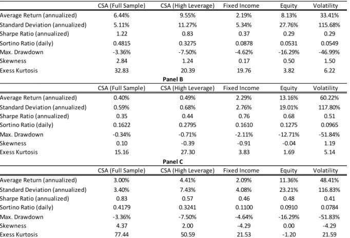
In this section we discuss the results of our strategy. We have implemented our strategy for three sets of companies based on their debt-to-equity ratio. For computational reasons, the survival probability was computed using the formula given by Finger et. al. (2002). Nevertheless, whenever the debt-to-equity ratio was found to be above the threshold provided by Kiesel and Veraart (2008), we turn to use the exact solution provided by the latter in order to calculate the model CDS spreads.

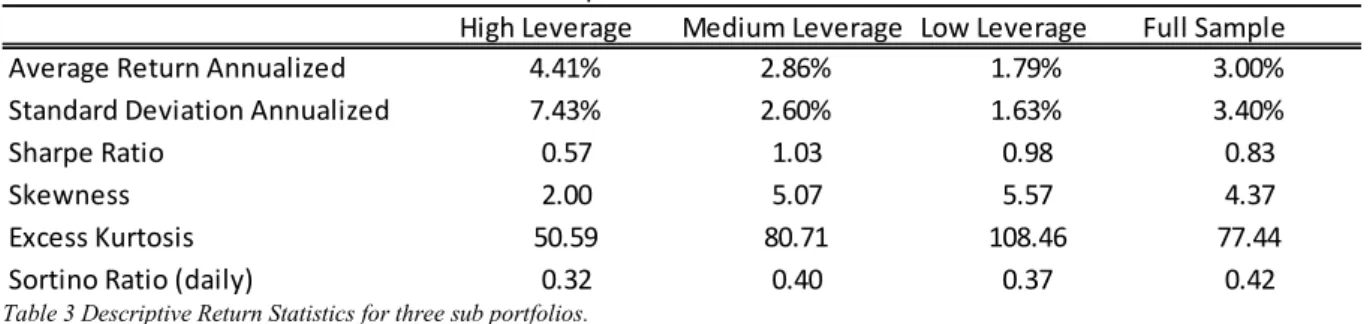
We have divided our sample of 67 companies in three different sub portfolios differing by the company average debt-to-equity ratio during the burn-in period (i.e. from 05.12.2007 – 04,12.2008).20_{. The “High Leverage”, “Medium Leverage” and “Low Leverage” portfolios are}

composed of 22, 23 and 22 firms, respectively. Table 3 presents some descriptive return statistics on all three portfolios. As one can see, the “Medium Leverage” portfolio outperforms all others in terms of Sharpe Ratio and Sortino Ratio. As literature suggests the CreditGrades model does not work well for very secure firms. In our case this can be seen in the very low annualized return of such companies. This outcome would be already expectable if we were trading with short – term maturities simply due to model misspecification. It is important to remind the reader that the CreditGrades model does not consider jumps. As such, it tends to produce very low spreads for short maturities in the case of very secure firms. This could lead our strategy to perform poorly. In our case, however, as we use 5 year CDS contracts, this could only be an issue in extreme cases such as L’Oreal, which has virtually no debt.

Table 3 Descriptive Return Statistics for three sub portfolios.

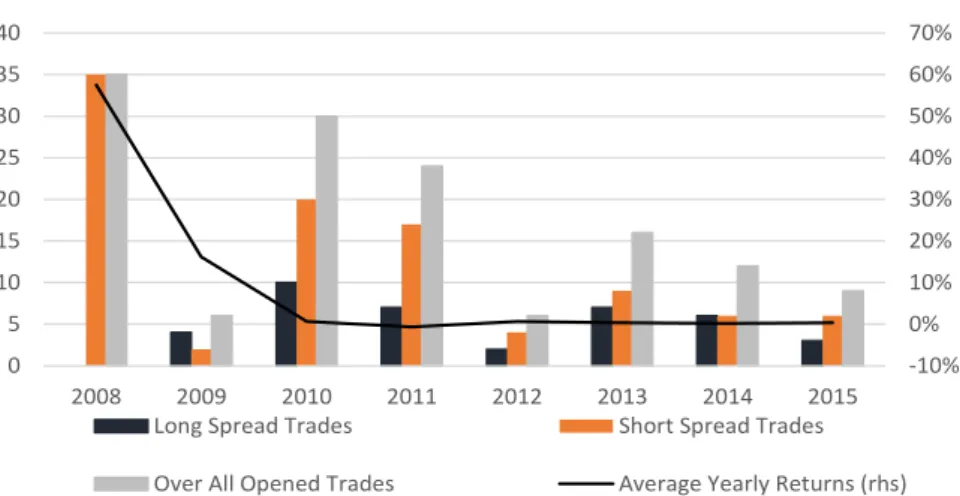
It is worth mentioning that our strategy is very dependent on trading opportunities, which seem not to be distributed evenly over time. The number of trades opened per year ranges between 3 (2012) and 35 (2008). Figure 4 shows a detailed split of opened trades per year as

20 _{Kiesel and Veraart (2008) use an equity to debt ratio, therefore a low ratio indicates an indebted company in}

their paper.

High Leverage Medium Leverage Low Leverage Full Sample

Average Return Annualized 4.41% 2.86% 1.79% 3.00%

Standard Deviation Annualized 7.43% 2.60% 1.63% 3.40%

Sharpe Ratio 0.57 1.03 0.98 0.83

Skewness 2.00 5.07 5.57 4.37

Excess Kurtosis 50.59 80.71 108.46 77.44

Sortino Ratio (daily) 0.32 0.40 0.37 0.42

29 well as the average performance for any given year. In 2008, the dominant strategy was to short CDS contracts (and equities). This can be explained with the course of the financial crisis. Notice that in 2008 CDS spreads exploded. In this context, our model has given strong signals to sell CDS contracts as this up rise was interpreted as some type of overreaction in CDS markets. In 2009 the number of trading opportunities diminished significantly with a slight bias in long CDS trades. We observed the highest return rates for our strategy during these two years. Following the sovereign debt crisis, trading opportunities emerged again in 2010 and 2011. Shorting CDS became again the dominant strategy. Returns were nevertheless low during this years as result of some sort of lead – lag relationship between the number of trades and returns. As credit spreads normalized in the following years, our model detected less trading opportunities. The years of 2013 and 2014 featured a fairly high number of buy protection signals and low returns. This should be related with the new environment within capital markets that followed the quantitative easing program implemented by the ECB, which contributed to depress credit spreads to all-time lows. According to our model, spreads then were too tight and therefore our model produced mainly buy protection signals.

Figure 4: Number of trades opened per year, split by nature of trades.

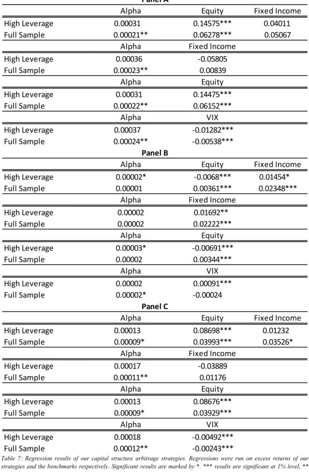
Since trading opportunities tend to cluster in time, it is important to examine trading returns for different sub periods. Table 6 shows some descriptive return statistics for the “High Leverage” and Full Sample portfolios against some benchmarks for different periods. As this is a “plug and play” trading strategy, we try to use only investable investment products as our benchmarks. The EuroStoxx ETF of Deutsche Asset Management and the iShares Euro Corporate Bond Large Cap ETF were used as our equity and fixed income benchmarks, respectively. Regarding volatility, the actual VIX Index on the S&P 500 was used, as there was

-10% 0% 10% 20% 30% 40% 50% 60% 70% 0 5 10 15 20 25 30 35 40 2008 2009 2010 2011 2012 2013 2014 2015

Trades Opened per Year

Long Spread Trades Short Spread Trades