Marketing
ISSN: 2146-4405
available at http: www.econjournals.com
International Review of Management and Marketing, 2020, 10(6), 58-78.
Demand Impact for Prices Ending with “9” and “0” in Online
and Offline Consumer Goods Retail Trade Channels
Marcial López-Pastor
1*, Jesús García-Madariaga
1, Joaquín Sánchez
1, Jose Figueiredo
21Faculty of Economics and Business Administration, Complutense of Madrid University, Spain, 2Instituto Politécnico de Santarém,
Portugal. *Email: [email protected]
Received: 07 September 2020 Accepted: 10 November 2020 DOI: https://doi.org/10.32479/irmm.10683
ABSTRACT
Studies on demand impact for 9-ending and rounded prices have so far offered controversial results, with hardly any research focusing on their effect on online commerce or in a multichannel sales context. Our study aims to fill this gap by analyzing the conditions that influence the strategy behind setting such type of pricing in the multichannel retail business of fast-moving consumer goods (FMCG). To test the formulated hypotheses, scanner data from FMCG retailers are used. In addition to “demand” and “price”, “promotion communication”, “retailer type” and “price level” are included as moderators between 9-ending, rounded prices and demand. The results aim to provide, both in the academic and business fields, systematic findings of pricing relationships between online and offline channels which contribute to a better management strategy for “9-ending” and “rounded” prices.
Keywords: Prices; 9-ending Prices; Rounded Prices; E-Commerce JEL Classifications: M31, L81, C32
1. INTRODUCTION
In today’s business environment with retail undergoing extraordinary changes offering consumers with new options in terms of what and where to buy (Gogoi, 2017), many researchers consider multichannel retailing to be highly profitable for businesses (Herhausen et al., 2015; Oppewal et al., 2013 Rangaswamy and van Bruggen, 2005; Wallace et al., 2004; Wind and Mahajan, 2002). Retailers are increasingly focusing on pricing strategies. By studying scanner data, it has been observed that demand elasticity was higher when shifting to a price ending with the number 9 than with any other digit (Blattberg and Wisniewski, 1983).
In traditional channels, many authors studied the variables’ significance of 9-ending and rounded prices for real demand compared to random prices (Blattberg and Wisniewski, 1987; Chu et al., 2008). Assuming price endings not only determined demand impact, although not homogeneously (Anderson and
Simester, 2003; Ngobo et al., 2010), factors such as promotion communication, product category, brand and even the country were analyzed, possibly explaining the variability in the impacts of 9-ending prices.
Regarding the effects of price endings on online channels, previous research yielded similar controversial conclusion (Melis et al., 2015) with few studies having explored these pricing strategies in an e-commerce context. The lack of research in such emerging markets was surprising given the changes to our understanding of business pricing and promotional processes due to the digital revolution (Chen et al., 2020; Misra et al., 2019).
It could be argued that the absence of comprehensive examinations in online markets could be explained by the less pronounced problems of price comparison by presenting fewer cognitive difficulties in memorizing and comparing products from different retailers (Hackl et al., 2014; Cebollada et al., 2019).
To the best of our knowledge, no one has delved into the relationship between price and demand at the three types of retailers based on the classification of Lee et al. (2009): (1) Brick and Mortar stores; (2) Multichannel (combining physical with online stores); and (3) Purely online (exclusively via the Internet) and the comparative effects among them.
The main objective of this study is to better understand the 9-ending and rounded pricing strategy, differentiating its use from offline to online channels and its influence on sales by analyzing the relationships between price and units sold. We examine the effects for the same product set sold at three type of retailers within the same time period with 9-ending prices in contrast with those ending with rounded numbers using their scanner data series according to the classification of Lee et al. (2009) of more than 60 products from leading manufacturers in the Spanish FMCG. As indicated by Levy et al. (2011) and Ater and Gerlitz (2017), if 62% of prices analyzed ended in 9 the remaining 38% were therefore randomly set. Moving to 9-ending prices led to about a 5 to 10% increase in sales (Anderson and Simester, 2003). Estimating the Spanish FMCG turnover to be around €53,636 million in 2019, the incremental impact could yield an increase between €800 million (+2%) and 1600 €million (+4%) in a market that grows at approximately 1.5% per year (Nielsen, 2019). Following Haupt and Kagerer (2012) who proposed a regression framework addressing price heterogeneity and promotional effects, time series regression models (TSML) are contrasted by types of Manufacturer Suggested Retail Price (MSRP) endings that are applied to scanner data series data with the objective of studying for each product the significance of 9-ending and rounded prices variables in real demand compared to types of random prices (Blatberg and Wisniewski, 1987; Chu et al., 2008). Other independent variables taken into consideration are “Retailer types,” “Group by MSRP levels,” and “Promotion Communication.”
The rest of the document is divided as follows: an overview of relevant literature is provided in section 2; followed by a detailed description of the problem and hypotheses statements in section 3; the research methodology is described in section 4; and the data used are listed in section 5, with a presentation of the results and a discussion in Section 6. Finally, the conclusions and future research are detailed in section 7.
2. THEORETICAL FRAMEWORK
The first scientific investigations reported by Ginzberg (1936) involved an experiment of a large mail order house in which results of sales and profits compared two groups of goods sold either with 9-ending or with rounded prices. The resulting profits for some products were considered unacceptable to the retailer. Final prices ending in 9 were common. Published studies indicated that between 30% and 65% of all prices ended in the digit 9 (Stiving and Winer, 1997; Schindler and Kirby, 1997; Blinder et al., 1998; Anderson and Simester, 2003; Levy et al., 2011; Anderson et al., 2015).
Nevertheless, there did not seem to be a consensus in the literature about what exactly constituted a 9-ending price especially when it came to more expensive items. The expanded definition included all prices ending in 9 in the cents position (Stiving and Winer, 1997). Other authors considered a price as ending in 9 only when it ended in 99 cents (Schindler, 2001), or if the last dollar digit was 9 (Anderson and Simester, 2003).
One alternative way defined the criteria they used for a range of items in different categories and that allowed them to define their price. 9-ending pricing referred to the use of prices that were below rounded prices, such as “9.99” instead of “10” or “99” instead of “100,” so they used the price endings “9 cents,” “99 cents,” and “9,” “9.99,” “99,” and “99.99” (Ngobo et al., 2010). (Mitra and Fay, 2010) used endings in 9 or endings in 0 according to the price level.
Results were divergent though. Most existing empirical research showed that in general, sale prices better explained the variability in consumer demand than other marketing-mix variables (Elrod and Winer, 1982; Stiving and Winer, 1997; Schindler and Kibarian, 1996; 2001). By studying scanner data, it was observed that demand elasticity was greater when scanned with a 9-ending price compared to any other one (Blattberg and Wisnieswski, 1983). Some studies suggested that the effects on sales for 9-ending prices were positive. For example, Nagle and Holden (1987) concluded that a brand’s sales increased by 194% when price dropped from 83 to 63 cents but increased by 406% when it went down to 59 cents. Blattberg and Wisnieswski (1987) examined the influence of 9-ending prices on a supermarket chain´s sales using scanner data. It was concluded that the effect was positive for thirteen out of the twenty-one brands suggesting that the impact of a final price ending in 9 differed between brands.
Some experiments conducted to understand the cognitive mechanisms of 9-ending prices yielded conflicting outcomes. Similarly, purchasing behaviors investigations produced mixed conclusions (Schindler and Kibarian, 1996). Noting that the variability due to price termination was incomplete, Anderson and Simester (2003) using actual sales, found that the final impact of the number 9 varied according to product awareness and the promotion materials used by retailers.
In addition, Bray and Harris (2006) reported sales growth for only nine out of ten products included in an experiment using data from retailers and found (Martínez-Ruiz et al., 2006) that 9-ending prices had no influence on sales. Furthermore, there was evidence that consumers preferred rounded prices (Lynn et al., 2013). They used price data set by consumers to pay for what they wanted to argue that consumers preferred even numbers although rounded prices were shown to have positively affected demand in a situation that encouraged the importance of convenience (Wieseke et al., 2016).
These investigations used pricing information and focused on analyzing consumers’ responses in this online market. However, they found it difficult to study the impact on demand because
in their sample they did not have the real demand for each type of price ending making it difficult for them to find the direct relationship. To the best of our knowledge, our work is the first to have a complete information base for both variables, examining this relationship in the online compared to the offline market, making this contribution robust both in the academic and business arenas.
The authors could not argue for an effect on a single sign and established hypotheses to dig deeper empirically in identifying the elements that could vary the effect of price endings. Baumgartner and Steiner (2007) argued that empirical results of a 9-ending price had a varying outcome according to categories such as chocolate drinks and notebooks for example, suggesting the need to explain the influence of other variables.
In addition, other research (Pauwels et al., 2007; Nijs et al., 2007) suggested that consumer response to 9-ending prices varied between categories depending on their nature or structure as well as store type. Store size affected products’ quantities and price ranges offered in each category to consumers (Ellickson and Misra, 2008; Hwang et al., 2010).
Ngobo et al. (2010) analyzed factors such as promotion communication and product category, concluding that prices ending in 99 attracted more buyers in more concentrated and higher promoted categories but fewer buyers in more expensive categories and brands.
Premium brands should be wary of using 9-ending prices because the impact was weaker for them and could lead to sales losses. On the contrary, they seemed very effective in increasing smaller brands’ sales in more affordable categories (Macé, 2012), and even the country, which could explain the variance in the influence of 9-ending prices.
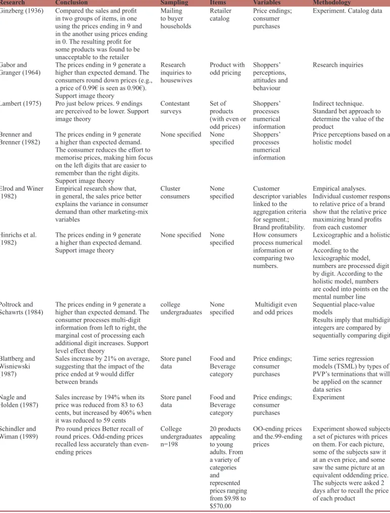
The characteristics of the retail trade arena could have ramifications in at least two ways: demography and competition (Chen et al., 2020; Misra et al., 2019; Vroegrijk et al., 2013). Research that several factors explain the divergent results found in the retail price suggested that response to consumer prices may also vary depending on (1) Promotion Communication, (2) Product Category, (3) Brand, (4) Retail Trade Characteristics, and (5) Country. In conclusion, studies carried out indicated that there was not a single reason for any price adjustment, but rather a great variety of theories (Liu et al., 2019; Cebollada et al., 2019; Salim et al., 2019; Wieseke et al., 2016; Hackl et al., 2014; Thomas and Morwitz, 2005; Bizer and Schindler, 2005; Schindler and Kibarian, 2001; Stiving, 2000; Gedenk and Sattler, 1999; Stiving and Winer, 1997; Schindler and Kirby, 1997; Schindler and Kibarian, 1993; Schindler and Wiman, 1989; Poltrock and Schawrts, 1984; Brenner and Brenner, 1982; Hinrichs et al., 1982; Lambert, 1975; Gabor and Granger, 1964) and factors to explain what has been observed (Table 1).
The Internet and social media emergence improved the dissemination of information on many of those elements especially price and competition in the marketplace, significantly changing
the means of communication between companies and consumers. With a world population of over 7.7 billion people, 59% use the Internet and about 3.8 billion or 49% of them are active on social media, a two-way communication means for companies to interact and receive instant feedback from customers and consumers. Arguably, the relationships among them could be enhanced to investigate the perceived risk by consumers influencing on consumer online shopping intention (Salim et al., 2019). However, the utilization of this new media requires a thorough understanding on how affected consumers could enhance business relationships for positive business outcomes as it is reflected by purchase intention and brand loyalty (Laksamana, 2020).
On the Web, consumers can now easily compare prices and track product information with price processing being much less expensive (Lee et al., 2009). It is feasible to think that customers act as multi-channel consumers, that is, they will use the two channels, combining them in the way that interests them most (Arce-Urriza and Cebollada, 2013).
Carpenter and Moore (2006); Teller et al. (2012) and Chintagunta et al. (2012) examined the influence of store attributes (price, product selection, atmosphere, etc.), focusing on analyzing the reasons for choosing the store format for supermarket products. On other aspects of channel choice and assuming that prices and promotions were the same for the two channels, Chintagunta et al. (2012) compared transaction costs derived from Internet purchases with the physical channels, concluding that they differed a lot. Each consumer, for each purchase, chose the channel that represented the lowest total cost and in this model the price was a variable with a lower impact on the purchase decision than in the traditional store, in part because 9-ending prices were rigid in the sense that price setters were more reluctant to change them. Levy et al. (2011) and Cebollada et al. (2019) concluded that for some product categories, there were households that showed less sensitivity to prices when buying online versus offline.
The lack of studies in emerging e-commerce markets could be argued considering the complexity of the business pricing process such as for example, the pricing decision of a manager at a large online retailer. In April 2019 Amazon.com had a total of 119,928,851 products, (https://www.scrapehero.com/how-many-products-does-walmart-com-sell-vs-amazon-com/- Accessed on August 11, 2020).
In these markets, managers must establish real-time MSRPs for each of these products. There are three characteristics that differentiate these environments from traditional retail channels. Firstly, given the number of products sold by large online retailers, pricing decisions need to be substantially automated (Misra et al., 2019). Specifically, it is not feasible for a manager to conduct market research, calculate price elasticity and establish optimal prices for each product (Baker et al., 2014). Secondly, online sellers can to modify prices almost continuously, and often randomize those changes for learning purposes. This differs from the traditional retail environment where retailers face high costs known as menu costs, to change prices by
Research Conclusion Sampling Items Variables Methodology
Ginzberg (1936) Compared the sales and profit in two groups of items, in one using the prices ending in 9 and in the another using prices ending in 0. The resulting profit for some products was found to be unacceptable to the retailer
Mailing to buyer households
Retailer
catalog Price endings; consumer purchases
Experiment. Catalog data
Gabor and
Granger (1964) The prices ending in 9 generate a higher than expected demand. The consumers round down prices (e.g., a price of 0.99€ is seen as 0.90€). Support image theory
Research inquiries to housewives
Product with
odd pricing Shoppers’ perceptions, attitudes and behaviour
Research inquiries
Lambert (1975) Pro just below prices. 9 endings are perceived to be lower. Support image theory
Contestant
surveys Set of products (with even or odd prices) Shoppers’ processes numerical information Indirect technique. Standard bet approach to determine the value of the product
Brenner and
Brenner (1982) The prices ending in 9 generate a higher than expected demand. The consumer reduces the effort to memorise prices, making him focus on the left digits that are easier to remember than the right digits. Support image theory
None specified None
specified Shoppers’ processes numerical information
Price perceptions based on a holistic model
Elrod and Winer
(1982) Empirical research show that, in general, the sales price better explains the variance in consumer demand than other marketing-mix variables
Cluster
consumers None specified Customer descriptor variables linked to the aggregation criteria for segment.; Brand profitability.
Empirical analyses. Individual customer response to relative price of a brand show that the relative price maximizing brand profits from each customer Hinrichs et al.
(1982) The prices ending in 9 generate a higher than expected demand. Support image theory
None specified None
specified How consumers process numerical information or comparing two numbers.
Lexicographic and a holistic model.
According to the lexicographic model, numbers are processed digit by digit. According to the holistic model, numbers are coded into points on the mental number line Poltrock and
Schawrts (1984) The prices ending in 9 generate a higher than expected demand. The consumer processes multi-digit information from left to right, the marginal cost of processing each additional digit increases. Support level effect theory
college
undergraduates None specified Multidigit even and odd prices Sequential place-value models Results imply that multidigit integers are compared by sequentially comparing digits
Blattberg and Wisniewski (1987)
Sales increase by 21% on average, suggesting that the impact of the price ended at 9 would differ between brands
Store panel
data Food and Beverage category
Price endings; consumer purchases
Time series regression models (TSML) by types of PVP’s terminations that will be applied on the scanner data series
Nagle and
Holden (1987) Sales increase by 194% when its price was reduced from 83 to 63 cents, but increased by 406% when it was reduced to 59 cents
Store panel
data Food and Beverage category Price endings; consumer purchases Experiment Schindler and
Wiman (1989) Pro round prices Better recall of round prices. Odd-ending prices recalled less accurately than even-ending prices College undergraduates n=198 20 products appealing to young adults. From a variety of categories and represented prices ranging from $9.98 to $570.00 OO-ending prices and the.99-ending prices
Experiment showed subjects a set of pictures with prices on them. For each picture, some of the subjects saw it at an even price, and some saw the same picture at an equivalent oddending price. The subjects were asked 2 days after to recall the price of each product
Table 1: Authors who empirically analyze the impact of prices ending in 9 and conclusions
Research Conclusion Sampling Items Variables Methodology
Schindler and
Kibarian (1996) + 8% sales increase Mailing to buyer households Clothes Price endings; consumer purchases Experiment. Catalog data Stiving and Winer
(1997) Positive effect of nine-endings on brand choice for yogurt data, negative effect for tuna sales
Consumer
panel data Yogurt and tuna Price endings; consumer purchases
Empirical analysis
Schindler and
Kirby (1997) Over representation of prices ending with 0, 5, and 9 found in retail advertising. Supports level effects Price announcements in newspapers. n=1415 None
specified 5 and 0-ending prices and the. 9-ending prices
Understatement effect Consumers will perceive that a final price of 9 is much lower than a final price of 0, which is actually only one unit higher
Blinder et al.
(1998) Final prices ending in 9 are common Large U.S. fi rms. n=200 Retail and nonretail industries
5 and 0-ending prices and the 9-ending prices
Descriptive study. 88 percent of firms in the retail industry and 47 percent in nonretail industries reported these kinds of price points in their pricing decisions Gedenk and
Sattler (1999) No significant differences for contingency factors. Odd-ending pricing strategy recommended for retailers’ adoption unless strong price-quality image effects exist
None specified None
specified Threshold prices. 9-ending prices Involvement. Not empirically tested
Schindler and
Kibarian (2001) Odd-ending pricing increased the likelihood of consumer judgment that an advertised price was low and discount-driven. Supports image effects Consumer panel. n=405 respondents Different product categories Consumer impression of the price discount based on the ending in 9 or 0, shown in the advertisement, and on each question in the survey Experimental data Anderson and
Simester (2003) 5-8% increase in sales, depending on the communication in promotion and the life cycle of the product
Compañías nacionales que venden por correo al por menor
Clothes Price endings; consumer purchases
Experiment. In this paper, a series of three field experiments are presented in which the price termination of many products is varied Bizer and
Schindler (2005) Pro just below prices. 9 endings are perceived to be lower. Consumers dropped off the rightmost two digits such that they showed greater purchase likelihood for products with odd-ending pricing. Supports level effects
None specified Hypothetical low-priced products Consumer difference variables. “processing motivation” in the underestimation effect Experiment Thomas and
Morwitz (2005) Increased preference for 9-endings importance of savings, time pressure, distance between prices, change in leftmost digit, limited information, hedonic consumption. Odd-ending pricing was more effective when the left-most digits differ. Supports level effects
Consumer panel respondents. n=102
None
specified The existence of the drop-off mechanism in price information processing
Experimental data. The respondents would be asked to provide estimates of how many of variously priced items they could purchase for $73.00
Bray and Harris
(2006) Pro round prices. Odd prices are less effective than round price, with trial sales, in nine of ten products. Women were more likely to respond favorably to odd-ending pricing than men. Supports image effects
Consumer panel data from supermarket UK
None
specified Price endings; consumer purchases
Store-based experiment
Martínez-Ruiz et al. (2006) Found that prices ending in 9 had no impact on sales. Furthermore, there is evidence that consumers prefer round prices
daily
store-level data None specified Price endings; consumer purchases
semiparametric regression model
Baumgartner and
Steiner (2007) People concerned about price should be more attracted by odd prices under greater time pressure
price (with five different levels) and brand name (with three different levels) Chocolate drinks and notebooks (computer) categories Consumer heterogeneity. (gender, individual participation and time pressure) Empirical evidence
Findings from a choice-based conjoint study with brand-price stimuli
Table 1: (Continued)
Table 1: (Continued)
Research Conclusion Sampling Items Variables Methodology
Nijs et al. (2007) The prices ending in 9 shown that consumer response varies among categories is likely to affect the results
Two different data sources: (1) store-level data from the Denver area. (2) store-level data from the supermarket retail chain Different product categories Retail prices, competitive retail prices and sales volume linked to retailer profitability Empirical analysis. multivariate time-series analysis Pauwels et al.
(2007) Consumer response to prices ending in 9 varies between categories depending on their nature or structure, as well as the store type
Scanner data from a supermarket for 399 weeks The top 4 brands across 20 fast-moving consumer good categories. Price elasticity of sales. Include: unit sales at the UPC level, retail price, price specials, promotions, and new product introductions
Empirical analysis. Smooth transition regression models to study threshold-based price elasticity.
Ellickson and
Misra (2008) The effect prices ending 9 could be due to the type of store that can affect the quantity of products and the price range offered in each category to consumers
Store level data set supermarket in the United States in 1998 Multiple product categories Pricing behavior: rival pricing, own pricing and other factor that influence (consumer demographics, rival pricing behavior, and market, chain, and store characteristics) Empirical analysis. System of simultaneous discrete choice models
Lee et al. (2009) Concluded that mixed retailers use 9-ended MSRPs much more frequently than the rest, being more popular for some product categories
Daily observations on categories sold by 90 Internet-based retailers collected over a two-year period. n=1.5 million Multiple product categories Store rating; Relative price; Popularity; Price length; Price level; Channel; 9 ending price
Empirical models for price-endings
Hwang et al.
(2010) The effect prices ending 9 could be due to the store size affects the quantity of the products and the range of prices offered in each category to consumers
Store-Level Scanner Data. 3040 stores, 52 weeks from the year 2005 The top-selling items from several product categories The dependence of assortment composition on customer, company and competition Empirical analysis. linear regression model Focus on modeling assortment similarity across pairs of stores
Mitra and Fay
(2010) They used endings in 9 or ending in 0 according to the price level. Those criteria that refer to this price range defined Comparative prices of identical products in different stores as reported by cnet.com. Several product categories. n=29 categories. Price to manage their customers’ service expectations Empirical analysis. Using a signaling model
Ngobo et al.
(2010) Significant, positive impact on the percentage of buyers. The effects on the SKU’s category choice are smaller in expensive categories
Consumer panel data for 156 weeks. n=11.000 SKU Several grocery products. n=103 categories
Unit sales, retail prices, and promotional activity at the SKU level
Conceptual model that incorporates the effects of nine end prices on brand choice
Levy et al. (2011) Find evidence that prices ending in 9 are rigid in the sense that price setters are more reluctant to change them
Two different data sources: (1) Consumer panel data from supermarket. (2) daily prices from the Internet on 474 products Across several product categories
Sale price; Unit sales.
Internet price information data
Probabilistic model of the likelihood of price changes To explore the contribution of 9-ending prices to price rigidity
Research Conclusion Sampling Items Variables Methodology
Macé (2012) Odd-ending prices selectively enhanced sales for small brands belonging to weaker categories, and lost their effectiveness as odd-ending pricing practices intensified. Supports both level and image effects Weekly, store-level scanner data from supermarket. 83 stores for 399 weeks Food and nonfood product categories. n=10
Log regular price; promotional activity.
The log price index captures: temporary price discounts, the log price indices of the main rival
Model sales responses to marketing mix variables. SCAN*PRO model, with its log–log specification
Lynn et al. (2013) Pro round prices consumers prefer
0-endings Two different data sources: (1) the payment sizes received for 65,535 PWYW purchases from 104 countries (2) sales and tip data from 9384 useable charge card receipts Computer game; Gratuity/ Tip Choices; Fuel Sales Data Prices Consumers’ choices across different pay that consumers chose to pay
Pricing model to test for consumer preferences for round numbers. It allows consumers to choose the prices they actually pay for goods and services
Vroegrijk et al.
(2013) The spatial dimension has a major impact on pricing strategies in at least two ways: demographics and competition. A pricing strategy may be a response to local competition
Consumer panel data from supermarket and Hard discounters Across several product categories
Unit sales; unit
sales private label Store choice and spending model that explicitly accounts for interstore synergies and multiple-store shopping behavior
Hackl et al. (2014) In online channel there are less pronounced problems of price comparison by presenting fewer cognitive difficulties in memorising and comparing products from different retailers. Supports level effect theory Price for 698 e-tailers and 23,317 products. N=805,949 Product offers whose average price is larger than €25, across several product categories Relative price of a firm’s price spell/the respective customer clicks on the product from the customers/ the time stamps/The following offer-specific/shipping time and cost
Empirical analysis. Explore the impact of these price points on the consumers’ demand
Anderson et al.
(2015) Online environment differs from the traditional retail where retailers face high costs to change prices, limiting the number of price changes
A record of every wholesale cost from a retailer and regular retail price change. 200 weeks Grocery, health and beauty, and general merchandise product categories
Cost and retail
price changes As a basis for comparison, calculate the probability of a price increase following a cost increase for items. linear probability model using OLS
Melis et al. (2015) Have found, regarding the impacts of price ending in online channel, the same controversial results examining these pricing strategies in the digital economy context
UK household panel over a two-year period, covering all multi-channel retailers Grocery
market. Using purchase data: Household category share/ Household brand share/Price/ Assortment Size/ Assortment Composition/ Price Integration/ Assortment Integration/Offline Store Preference/ Online Loyalty
Online store choice model multinomial logit model to analyse online store choice, its underlying drivers and the moderating effects of experience
Wieseke et al.
(2016) Round prices are shown to positively affect demand in a situation that encourages the importance of convenience Two data sources: (1) Customers (2) consumer panel Takeaway good; Consumer durable; Consumption goods Price endings/ Actual sales/ Convenience consciousness/Price attractiveness/ Price convenience/ Follow-up/ Transaction convenience Reaction time/ Purchase intention To enhance understanding of the effects of price endings on sales by examining the question of whether consumers’ convenience consciousness impacts their judgment of price endings
limiting the number of price modifications (Anderson et al., 2015). Lastly, because of the difficulty in setting prices due to the existence of online sales models through agencies that prevent the control of final prices to manufacturers (Chen et al., 2020).
The scarcity of studies in emerging e-commerce markets could be also argued considering the promotional process. Online promotion channels were widely used by businesses to stimulate sales in retail. (Chen et al., 2020). This could be explained by the less pronounced problems of price comparison by presenting fewer cognitive difficulties in memorizing and comparing products from different retailers (Hackl et al., 2014).
The absence of research in emerging e-commerce marketplaces is surprising given that the digital revolution is changing our understanding of the academic literature research and companies’ pricing processes.
3. HYPOTHESES
Investigations of the effect of 9-ending prices and round prices on sales applied different methodologies (field testing, consumer surveys and scanner data analysis) in different markets (food, women’s clothing, services) and considered the impact in a single sales channel (traditional physical store channel, catalog or internet sales, among others) (Anderson and Simester, 2003; Martínez-Ruiz et al., 2006; Bray and Harris, 2006; Schindler and Kibarian, 1996; Nagle and Holden, 1987; Blattberg and Wisniewski, 1987). Hackl et al. (2014) analyzed the problem in the context of e-commerce, a highly competitive and transparent environment with price comparison sites that on the outset were not considered very favorable to price points. Findings were consistent with Basu (2006) who assumed that strictly rational buyers ignore the digits on the right due to limited processing capacity and therefore companies in this context will also adjust to this behavior by establishing prices that end in 9.
Research confirmed the importance of 9-ending and rounded prices in different distribution channels, physical and digital (Misra et al., 2019; Baker et al., 2014) but without obtaining a comparable measurement of the impact on demand among them. Thus, the hypothesis to be tested would be the following:
H1-The influence of prices “9-ending” and “rounded numbers” on the real demand of end consumers is the same in online and offline groups of products in the consumer goods market.
In cross-sectional pricing and promotional studies (Vroegrijk et al., 2013; Hwang et al., 2010; Ellickson and Misra, 2008; Baumgartner and Steiner, 2007; Ailawadi et al., 2006; Macé and Neslin, 2004; Anderson and Simester, 2003; Bell et al., 1999; Narasimhan et al., 1996; Hoch et al., 1995), key factors related to elasticities such as store typology, category and product characteristics emerged for retail managers and academics.
In the case of 9-ending prices, there were studies showing that consumer response varied among categories and was likely to
affect the results (Pauwels et al., 2007; Nijs et al., 2007), as well as between the price level of the brands as indicated by Macé (2012) and Ngobo et al. (2010), who concluded that 9-ending prices seemed more effective in increasing sales of smaller brands in affordable categories.
This impact variation was observed in a type of physical stores where assortments and stocks were limited, focusing on the product category’s role. Dhar et al. (2001) told us that the optimal pricing strategy may differ if the retailer chooses to stock products at all price points but we have not determined if such a variation occurs similarly in the online market in which, as we have seen (Cebollada et al., 2019; Arce-Urriza and Cebollada, 2013; Teller et al., 2012; Chintagunta et al., 2012; Carpenter and Moore, 2006), the purchase criteria may change and the category under study is likely to affect the results. Therefore, the hypothesis to be tested would then be the following:
H2-The impact on demand of 9-ending and rounded prices is not the same among products of different price levels in different categories for a given distribution channel.
4. METHODOLOGY
4.1. Sampling
The objective of this study is to test the hypotheses with information of “real demand” for each “price type.” As Little and Ginese (1987) and Blattberg and Wisnieswski (1987) have done, we work with temporary series of scanner data on which linear regression models are applied to look for the effect of 9-ending prices.
Like many price studies, this research examines prices of products sold at supermarkets. Based on Nielsen’s hierarchy for the FMCG market in Spain, the main references of manufacturers positioned at the top of their categories are considered which represent 79% of the total Spanish 2019 FMCG market (Appendix 1) and to each of the 3 main segments: Food and Beverages (63.7%), Fresh Produce (15.2%) and Perfumery Drugstore (21.2%). The number of products analyzed (Number of Items) as well as the observations obtained in the sample for each of the three categories (Number of Obs.) has a similar proportion with the representation of each one in the market (Table 2).
Almost exclusively for this study, three different types of retailers are considered for their consumer sales channels: Mixed, Pure Offline and Pure Online (Table 3).
For uniformity purposes, the scope referred to was the Community of Madrid Region, representing 13% of the total Spanish market and in which the three types of retailers compete, given the development of “online” in mass consumption is limited to a province/region as it was subject to logistical restrictions (e.g. “tudespensa.com” only operates in Madrid).
The spatial dimension had a major impact on pricing strategies in at least two ways, demographics and competition. A pricing strategy may be a response to local competition (Vroegrijk et al.,
Table 2: Summary by product category
Category Number_of_Items Number_of_Obs Mean_Price Std_Dev Min_Price Max_Price
Food and beverages 40 1,902,626 1,523,810 0.7742177 0.12 7.50 Drugstore and perfumery 15 499,635 2,296,880 1.1631058 0.14 7.59 Fresh produce 16 651,853 2,089,714 0.5797970 0.28 3.95
Source: Nielsen, 2019
Table 3: Registry numbers by retailer type
Type of distribuidor Retailer name Number_of_Obs Percentage
Retailer mixed Dia% Supermercados. 2,390,442 78 Retailer offline Supermercados Hiber 546,963 18 Retailer online Tudespensa.com 116,709 4
Source: Nielsen, 2019
2013; Gourville and Moon, 2004). It is proposed that the retailer type aggregation criterion should be the “Postal Code,” otherwise, as in the case of the online retailer, there would only be a single store. Using the Postal Code, there are as many tudespensa.com online stores as there are Postal Codes wherever they had delivered an order (Table 4).
Store size affected the quantity of products and the range of prices offered in each category to consumers (Ellickson and Misra, 2008; Hwang et al., 2010). For this reason, it is necessary to focus the study on same store formats (supermarkets) with similar price positioning (private label present as first price and manufacturer name brand as premium), assortment (limited selection with reduced spaces), and promotion (more frequent promotions Temporary Price Discount versus Hyper with promotions that increase the amount by purchasing actions, for example: 3 for 2, second unit at 70% off, etc.) (Kantar world panel, 2014). Size and business format of the selected online and mixed retailers are classified in the supermarkets (Nielsen) segment, which represented 45% in value (turnover in euros) of the market in the selected Madrid area. Both retailers represente around 20% of the supermarket business segment in Madrid (Nielsen, 2019). If we review possible factors that influenced the impact of price endings collected in the literature, in our study we focus on the characteristics of retail trade (channels Off, On or Mixed), product category (Price level) and communication of the promotion (Temporary price reduction). We do not include in our analysis the brand, because we consider that the brand’s positioning and image are the same regardless of the offline and online channel and country. Due to the uniformity of the main variables of the study, our focus is on a region where the three types of distributors operate.
Another possible concern with sample representativeness might be the small number of products that are analyzed (63 products) in the panel data analysis, compared to hundreds of products in other studies. For example, Chakraborty et al. (2015) tracked 370 products, and Levy et al. (2015) also covered a considerably larger number of products. Although this sample might be considered a limitation of this research, it is necessary to highlight that, in comparison with other studies, the pricing behavior of the same products is analyzed in three different types of retailers (offline,
online and mixed) in a same period over 2 years (2017 and 2018). Other studies, despite analyzing a greater number of products, were only able to examine the behavior of prices at a specific time. For example, in Levy et al. (2011), for grocery price data, there was a maximum of four prices for the same product at any given time. The two main reasons why the products sample addressed in this analysis is representative of the FMCG universe are: Firstly, the price distribution with special endings is similar to the comparable distributions found in other studies. For example, we found that in this study, 59% of prices ended with “5” and “9,” with prices ending in “9” in the research of Levy et al. (2011) and Ater and Gerlitz (2017) being at approximately 62%. Secondly, as in the aforementioned investigations, terminations “0”, “5” and “9” are the most common ones. In this study, they reached 62%, being 70% and 71% for the offline and online retailers respectively. In order to have a better adjustment, information used in the product detail was collected on a daily basis since it was at such a level that the real price (in decimals) paid by the consumer could be identified. The sample period is two years for achieving the data volume necessary for any regression exercise that considers the interaction between seasonality-trend, both in examining price distribution formats as well as by store or category.
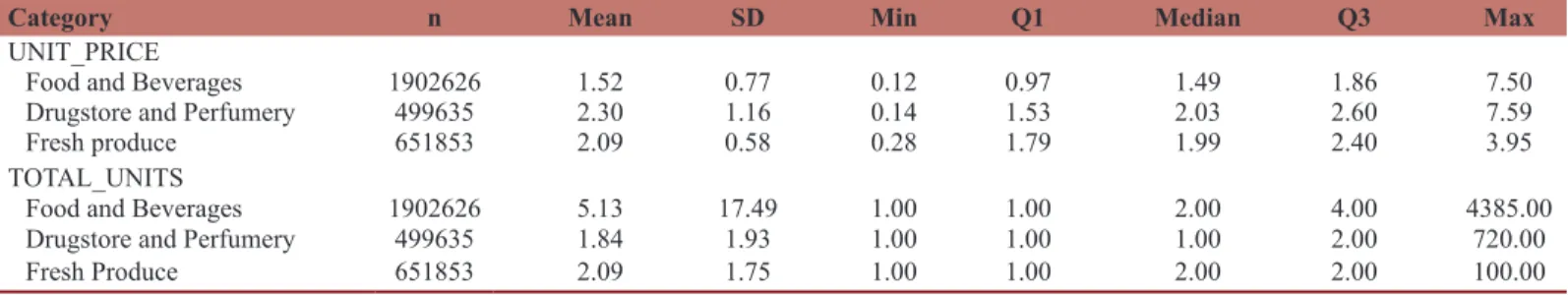
Once these external variables are generated, those variables of interest are selected (Table 5) and a system was developed to collect and integrate the information from the different retailers of the Spanish FMCG market included in this study. Table 6 below provides the descriptive analysis of the numerical variables Unit Price and Total Units.
The statistics of the numerical variables by Channel and the statistics of the numerical variables by Product Category are presented in Tables 7 and 8 respectively. The number of different label factors for each categorical variable is shown in Table 9. In this research, the Unit Price considered was the retail price at which the product was purchased. This price includes the Value Added Tax (VAT). Prices are the actual transaction prices recorded by the chain’s scanners (Levy et al., 2011). Given that low priced products are analyzed, the maximum price is 7.59€, all being below 10€; those criteria that refer to this price range of those defined by Mitra and Fay (2010) apply.
Therefore, in this analysis a price ends in “9” when: 1. It ends in 99 cents: 0.99€, 5.99€
2. Being less than 10€ and contains a 9 in the cents position: 0.59€, 2.19€, 7.59€
3. For numbers greater than 10€ that have a 9 in the unit position and without cents: 19.00€, 29.00€.
If a price does not end in “9,” it is considered as ending in “0” if: 1. It is less than 10€ with a zero in the cents position: 0.90€, 4.20€ 2. It is less than 10€ and it ends without cents: 1.00€, 2.00€, 7.00€ 3. For numbers greater than 10€ that have a “0” in the unit
position and without cents: 20.00€, 30.00€.
If a price does not have an ending in “9” or an ending of “0,” it is classified as having a “random” ending.
Based on this classification, there were prices with “9” endings, “0” endings and a “random” ending in each of the data sets. Demand was defined by the number of units that consumers purchased of the product under study, in the different sales channels to which it has access and in which it can be found. Price is included as the independent variable along with other variables that will attempt to explain its impact on demand (Mitra and Fay, 2010).
Two independent variables are also considered:
“Promotion Communication” (1); Schindler (2006) discussed the more general market relationship between termination in 9 and the presence of a claim that the advertised item is sold at a reduced price that could be communicated via catalogue, the web, press, at the establishment and even in the product packaging itself. This variable will take a value of “1” if the final price to the consumer is promotional (when it is accompanied by a message to the consumer during a specific period) that offers the customer a sales advantageous situation and “0” in the event that there is no message. “Type of Retailer” (2); Lee et al. (2009) classified them into three types according to how they combine in their distribution network: online, offline and mixed sales channels. This variable will take the value “Offline” when the retailer only has physical stores, “Online” if only present on the internet and “Mixed” when both channels are combined.
4.2. Data
Like Haupt and Kagerer (2012), an empirical analysis is carried out to model the response of sales using data from consumer goods
Table 7: Statistics of the numerical variables by channel
Channel n Mean SD Min Q1 Median Q3 Max
UNIT_PRICE MIXED 2390442 1.75 0.86 0.12 1.21 1.69 2.10 7.50 OFFLINE 546963 1.86 0.97 0.26 1.25 1.79 2.09 7.35 ONLINE 116709 1.80 0.86 0.53 1.25 1.79 2.29 7.59 TOTAL_UNITS MIXED 2390442 3.73 14.33 1.00 1.00 2.00 3.00 4385.00 OFFLINE 546963 5.23 13.42 1.00 1.00 2.00 4.00 614.00 ONLINE 116709 2.26 4.68 1.00 1.00 1.00 2.00 588.00
Table 8: Statistics of the numerical variables by product category
Category n Mean SD Min Q1 Median Q3 Max
UNIT_PRICE
Food and Beverages 1902626 1.52 0.77 0.12 0.97 1.49 1.86 7.50 Drugstore and Perfumery 499635 2.30 1.16 0.14 1.53 2.03 2.60 7.59 Fresh produce 651853 2.09 0.58 0.28 1.79 1.99 2.40 3.95 TOTAL_UNITS
Food and Beverages 1902626 5.13 17.49 1.00 1.00 2.00 4.00 4385.00 Drugstore and Perfumery 499635 1.84 1.93 1.00 1.00 1.00 2.00 720.00 Fresh Produce 651853 2.09 1.75 1.00 1.00 2.00 2.00 100.00
Table 5: Variables of interest
EAN Product identifier
POSTAL_CODE Store location identifier CHANNEL Retailer type
DATE Sales date (daily level) UNIT_PRICE Unitary sales price TOTAL_UNITS Total units sold
PROMO Sale on promotion (yes/no)
Table 4: Postal code numbers by retailer type
Retailer type Retailer name Number
Retailer mixed Dia% Supermercados. 89 Retailer offline Supermercados hiber 23 Retailer online Tudespensa.com 264
Table 6: Descriptive analysis of the numerical variables unit price and total units
Variable n Mean SD Min Q1 Median Q3 Max
UNIT_PRICE 3054114 1.77 0.88 0.12 1.22 1.73 2.1 7.59 TOTAL_UNITS 3054114 3.95 13.93 1.00 1.00 2.00 3.0 4385.00
Table 9: Number of different label factors for each categorical variable Count_Factors EAN 71 POSTAL CODE 280 CHANNEL 3 DATE 728 PROMO 71
scanners. The information is collected and integrated from the different FMCG retailers in the Spanish market included in the study aligning them at product level (EAN code).
To test the hypotheses, we used daily purchase scanner data at each physical store or postal code delivered level from three retailers in the consumer goods market (one Online, another Offline and the third Mixed) of a set of 63 products (representing all mass consumption categories in Spain), with sales in the three retailers during the same time frame and in the same geographical area over a two-year period: 2017 and 2018. A total number of transactions of 3,054,114 was registered from 2017-01-02 to 2018-12-31. Retail scanner data, provided by Information Resources Inc. (IRI) and Nielsen, was the primary source of data for analysis in the packaged consumer goods industry due to the immediate availability of item-level data on factors such as price, quantity, promotional activity and sales channel. (Blattberg and Neslin, 1987; Stiving and Winer, 1997; Macé, 2012). The disadvantage of these sources was they only recorded sales in the physical stores of the main retail chains in Spain and did not audit sales in the Online channel. In this work on pricing behavior in main retail channels, data on own cash outlets provided by each of the three selected retailers are used to construct a disaggregated cross-section of data on daily purchase at each point of sale or postal code.
At that point, it is ruled out to continue with the study of “MSRPs ending in 0” since their percentage is very low with respect to the rest of MSRP types depending on their ending (Table 10). For uniformity purposes, products included in the study must have sales at all the retailers during the same time period and in the same geographical area, avoiding differences between the strategies over time or differences between stores due to their locations. The “private label” store brand assortment was removed from the analysis. With this, in addition to ensuring that the study allows for a comparative analysis “among retailers” for a set of items sold in the three target retailers (offline, mixed and online) in the same period analyzed, it also eliminates the bias that can be caused by the fact that private label consumers are more price sensitive and 9-ending MSRPs are expected to have a lower effect than for
those products sold under manufacturer name brands (Ailawadi et al., 2001; Narasimhan et al., 1996).
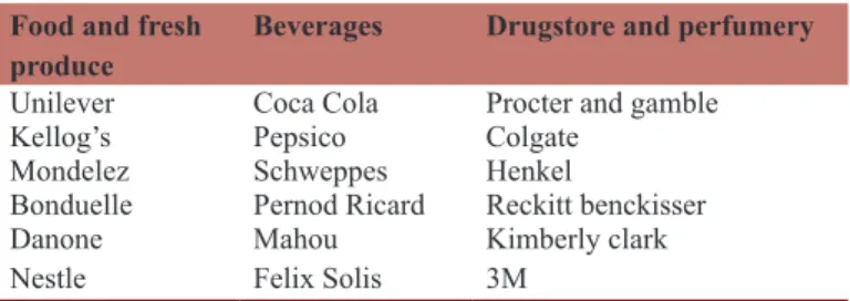
With this methodology, variables are kept constant and the impact of common variables on real sales in the three distribution channels analyzed. The number of products studied in the period was 71 in the mixed channel, 66 in the Offline and 63 in the Online, belonging to both national and multinational manufacturers (Table 11). Therefore, the examined set is of the 63 products common to the three types of retailer at EAN code level, representative of the top 3 in sales of thirty different product categories according to the Nielsen hierarchy. It has been chosen to explicitly incorporate this source of heterogeneity hoping to have different results with respect to the pricing strategy at category level (Appendix 1). For the analysis and testing of hypotheses at the aggregate level by type of retailer and product category, all items available in each of them will be used (Appendix 2).
4.3. Model
The main objective of this research is to develop a model that relates the demand for the product to its price. For each reference with prices ending in 9 and with other prices, the relationships between the variables price and demand in each type of retailer, price level and promotion is examined. Blattberg and Wisniewski (1987) and Schindler and Kibarian (1996) describe a model that relates price and other factors to sales of items from a supermarket. Kashyap (1995) and Bergen et al. (2005) studied these relationships, also considering the application of discounts in greater or lesser frequency over time and with different depths. Following Haupt and Kagerer (2012), who proposed a regression framework that allowed the direct estimation of price impacts addressing the heterogeneity of prices and promotional effects, models are contrasted by type of MSRP endings. In contrast, a time series regression model (TSML) is compared since they will be applied on laser data from scanner in order to study for each product the statistical significance of the price variables ending in 9 in real demand as opposed to types of random prices (Blattberg and Wisniewski, 1987; Chu et al., 2008), for three types of retailers depending on their sales channels. Therefore, other regression models focused on real demand prediction according to price type. TSLMs are predictive models that combine the interaction between seasonality trends and other regressions. A linear time series model provides a direct way to find a method to generate predictions of future values of the time series given the observed values of measuring the uncertainty of the predictions and being
Table 10: Percentage with respect to the rest of MSRP types depending on their ending
MSRP n %
0 108,575 4
Rest 2,945,534 96
Table 11: Manufacturers of studied products
Food and fresh
produce Beverages Drugstore and perfumery
Unilever Coca Cola Procter and gamble Kellog’s Pepsico Colgate
Mondelez Schweppes Henkel
Bonduelle Pernod Ricard Reckitt benckisser Danone Mahou Kimberly clark Nestle Felix Solis 3M
a dynamic task of updating by weighing more closely the data closest in time to the predicted values (Peña et al., 2001). Thus, the best econometric model must be adjusted regularly to generate optimal forecasts (Evans, 2003).
In addition to the fact that the time series model offers, in a simple way, a price-demand relationship, which is exactly what is sought (prediction capacity is not pursued), we do not apply ARIMA models because in order to apply the ARIMA methodology the time series must be stationary, that is, the mean and variance do not vary with time nor do they follow a trend (De Arce and Mahía, 2003).
The time series on which this study is supported cannot be considered stationary because the variance is not constant over time. This is normal for high frequency series where the data is less than the monthly period and the variance changes over time alternating periods of high volatility (high variance) with periods of low volatility (low variance) in a non-systematic way (Rayhaan, 2011).
The criterion of grouping prices based on the monetary amount makes empirical sense since in many studies carried out, they emphasized that the impact of those ending in 9 depended on the category’s price level. Macé (2012) performed an empirical analysis using consumer goods scanner data to model nonlinearity in sales response by grouping them into three price level segments. Haupt and Kagerer (2012) in a similar study, ranked them as Premium, Mid-priced and Low-Price Segments.
A segmentation analysis of the Unit Price variable is performed to identify the products positioning studied according to their price, using a K-means analysis to find the group that results in well separated compact groups. The objective is to minimize this measure since we want to reduce dispersion within the group and maximize separation between groups (Bezdek and Pal, 1998).
To do this, price (Unit Price) and sales (Total Units) are added weekly and by cluster type of product MSRPs. Following the literature, we make an approximation of K = 3 (High, Medium and Low Price) and observe that the “High Price” group contains few records compared to the other groups (1.1%) and causes no models to be generated for this cluster, preventing the interpretation of the demand relationship for that group of products.
In order to increase observations and improve interpretation (Peña et al., 2001), the analysis was performed with K = 2 and the result indicates that the means of the price factor were significantly different (P < 0.05) for the two clusters so the number of clusters is left at 2, verifying that the number of models that could be obtained increased (Table 12).
This way, a price segmentation is achieved with which to categorize the products as “MSRP_Low” and “MSRP_High”, generating a third independent variable called “Group by MSRP” that allowed for a better behavior understanding with respect to each group. This variable took “MSRP_Low” value when the product is in a low MSRP cluster below 2.22€ and “MSRP_High” if it belongs to the high MSRP cluster above said price. This grouping implies that independent variables defined above would add the “MSRP Cluster” of the product (low/high).
This made it possible to apply TSLM models separated by “price endings” (MSRP ending in 9 or MSRP other endings) for each item (EAN) on weekly data series considering as independent variables “Unit Price,” “Retailer Type,” “Promotion” and also the “MSRP Cluster.”
Since our methodology is based on making models by type of MSRP endings, the weekly aggregation will be made after having separated the models by “endings of MSRPs” (ending in 9, 0 or random). Therefore, it only considers a type of MSRP in these aggregations and ensures that this weekly aggregation does not penalize the number of records for the model.
The model presents the following equation:
∆ Demandtijkl = φ0 + φ1Tti + φ2Sti + β3 PVP end x_tijkl + ε ∆ = Statistical variation T = Trend S = Seasonality Β = Elasticity coefficient ε = Statistical error t = Period i = Item j = Retailer type k = Promotion l = MSRP cluster
Relationships between variables and their significance are studied so that the coefficient of determination (R2) is of relative importance
in the results. What matters is the variables’ significance value. Considering the defined price segmentation (K-means analysis, K=2) the following volumes are obtained per model (Table 13). With this modelling, the model combo is expanded by weekly records (16 models) although those below 104 weeks (8 models) would continue to be discarded to ensure the complete availability of weekly information for the study period.
5. RESULTS
This study examines the impact on real demand of 9-ending prices and the difference between retail level clusters and product Table 12: Product cluster analysis results
Cluster Cluster is comprised of products which have Min. 1st Qu. Median Mean 3rd Qu. Max.
1 MSRP_Low 0.120 1.090 1.510 1.438 1.800 2.221 2 MSRP_High 2.230 2.490 2.750 3.008 3.190 7.590
categories in different sales channels based on real data from each of the three retailers. The results respond to the existing gap in the relationship of prices with real demand for consumer products in the online channel. This study is the first to directly examine the effect of 9-ending prices on a wide range of product categories that share online sales and traditional formats.
It was analyzed from a double focused approach. A first in which we model with the defined equation that introduces as independent variables price, retailer type, promotion and segmentation by price cluster. A second in which we add the products category according to the Nielsen categorization for FMCG.
5.1. Focus 1
Models development including the level by Cluster of MSRPs, in addition to price, promotion and retailer type. The outcome is shown below with the components of each model (Table 14).
The results obtained in this study show that prices ending in 9 are significant in the three types of retailers. Our study shows that they are more relevant in the offline channel (P = 0.000004) and in the mixed channel (P = 0.000007) than in the online channel (P = 0.009090). This difference can be explained by the less pronounced problems of price comparison that Hackl et al. (2014) pointed out. It could also be due to the type of stores that can affect the quantity of products and price range offered in each category to consumers (Ellickson and Misra, 2008; Hwang et al., 2010).
The results proved that, just like Blattberg and Wisniewski (1987), demand elasticity was greater when passed at a price ending in 9. However, results were divergent, being more significant for the “Low MSRP” group products when it is confirmed that 9-ending prices influence demand, not for “High MSRP” products at any type of retailer. The results of the investigation validate as Macé
Table 14: Results of the first approach models
Terms model Mod 1 Mod 2 Mod 3 Mod 4 Mod 5 Mod 6 Mod 7 Mod 8
(Intercept) 2.664** 1.933* 29.354*** 3.466*** 24.786*** 2.092 26.979 1.843 Conf.Int [0.908, 4.420] [0.025, 3.841] [20.123, 38.585] [1.627, 5.305] [11.856, 37.716] [−0.261, 4.447] [−17.426, 71.384] [−1.749, 5.435] t (3.165) (2.113) (6.633) (3.931) (3.998) (1.860) (1.267) (1.070) Price −0.384 0.199 −18.346*** −0.688* −14.638** 0.128 −16.536 0.049 Conf.Int [−0.978, 0.208] [−0.969, 1.369] [−24.710, −11.983] [−1.308, −0.069] [−24.101, −5.174] [−0.449, 0.705] [−47.100, 14.027] [−1.126, 1.224] t (−1.352) (0.356) (−6.014) (−2.320) (−3.226) (0.465) (−1.128) (0.087) N 74 74 74 74 74 73 74 74 R2 0.909 0.853 0.930 0.851 0.825 0.574 0.657 0.830
Table 13: Volumes obtained per model considering the defined price segmentation (kmeans analysis K = 2)
Model Retailer MSRP Promotion Cluster Total Weekly
Mixed_9_0_MSRP_High Mixed 9 0 MSRP_High 154841 106 Mixed_9_0_MSRP_Low Mixed 9 0 MSRP_Low 513672 106 Mixed_9_1_MSRP_Low Mixed 9 1 MSRP_Low 113511 106 Mixed_RANDOM_1_MSRP_Low Mixed RANDOM 1 MSRP_Low 278956 106 Mixed_RANDOM_0_MSRP_Low Mixed RANDOM 0 MSRP_Low 1072808 106 Mixed_RANDOM_0_MSRP_High Mixed RANDOM 0 MSRP_High 248382 106 Offline_9_0_MSRP_Low Offline 9 0 MSRP_Low 176179 106 Offline_9_0_MSRP_High Offline 9 0 MSRP_High 65880 106 Offline_RANDOM_0_MSRP_Low Offline RANDOM 0 MSRP_Low 251628 106 Offline_RANDOM_0_MSRP_High Offline RANDOM 0 MSRP_High 52743 106 Online_9_0_MSRP_Low Online 9 0 MSRP_Low 21175 105 Online_9_0_MSRP_High Online 9 0 MSRP_High 12172 105 Online_RANDOM_0_MSRP_High Online RANDOM 0 MSRP_High 12671 105 Online_RANDOM_0_MSRP_Low Online RANDOM 0 MSRP_Low 59564 105 Mixed_RANDOM_1_MSRP_High Mixed RANDOM 1 MSRP_High 27131 104 Online_RANDOM_1_MSRP_Low Online RANDOM 1 MSRP_Low 5875 104
Terms Model Mod 9 Mod 10 Mod 11 Mod 12 Mod 13 Mod 14 Mod 15 Mod 16
(Intercept) 22.535*** 2.690*** 15.924 1.741 6.636*** 1.398*** 2.390*** 7.730* Conf.Int [16.121, 28.949] [1.801, 3.579] [−5.862, 37.710] [−0.615, 4.098] 10.024][3.248, [0.689, 2.107] [1.326, 3.455] 14.322][1.138, t (7.329) (6.310) (1.524) (1.546) (4.099) (4.128) (4.701) (2.454) Price −11.625*** −0.225 −5.109 −0.087 −2.854** −0.053 −0.372* −3.843 Conf.Int [−15.472, −7.777] [−0.527, 0.076] [−21.854, 11.634] [−0.969, 0.795] [−4.912, −0.797] [−0.201, 0.094] [−0.718, −0.025] [−8.819, 1.133] t (−6.302) (−1.557) (−0.636) (−0.206) (−2.904) (−0.756) (−2.246) (−1.616) N 74 74 74 73 73 73 73 73 R2 0.924 0.895 0.877 0.763 0.878 0.764 0.769 0.853 ***p<0.001; **p<0.01; *p<0.05
Table
15: Results of the second appr
oach models Terms model Mod 1 Mod 2 Mod 3 Mod 4 Mod 5 Mod 6 Mod 7 Mod 8 Mod 9 Mod 10 (Intercept) 3.366** 2.569*** 2.723*** 5.803*** 3.404*** 4.935 22.595*** 1.069 2.873*** −4.399** Conf.Int [1.304, 5.428] [2.265, 2.872] [1.882, 3.563] [4.005, 7.601] [1.584, 5.225] [−1.623, 1 1.494] [13.382, 31.809] [−0.293, 2.433] [2.030, 3.717] [−7.002, −1.796] t (3.405) (17.645) (6.759) (6.732) (3.914) (1.569) (5.1 15) (1.637) (7.104) (−3.525) Price −0.626 −0.339 *** −0.481 ** −2.278 *** −0.609 −1.552 −15.195 *** 0.093 −0.582 *** 2.302 *** Conf.Int [−1.359, 0.107] [−0.435, −0.243] [−0.783, −0.179] [−3.471, −1.084] [−2.275, 1.056] [−4.941, 1.835] [−22.270, −8.1 19] [−0.304, 0.491] [−0.867, −0.297] [1.327, 3.278] t (−1.780) (−7.379) (−3.321) (−3.981) (−0.766) (−0.955) (−4.479) (0.490) (−4.259) (4.925) N 74 74 74 74 73 74 74 74 74 74 R 2 0.915 0.944 0.885 0.858 0.903 0.763 0.915 0.883 0.870 0.917 Terms Model Mod 1 1 Mod 12 Mod 13 Mod 14 Mod 15 Mod 16 Mod 17 Mod 18 Mod 19 Mod 20 (Intercept) 31.810*** 1384 −0.617 9.903 3.184** 2.281** 0.153 2.236*** −9.528** 17.622*** Conf.Int [17.635, 45.985] [−1.267, 4.036] [−3.366, 2.130] [−34.039, 53.846] [1.463, 4.905] [0.770, 3.792] [−2.853, 3.159] [1.293, 3.180] [−14.758, −4.298] [9.035, 26.208] t (4.681) (1.089) (−0.468) (0.470) (3.872) (3.160) (0.106) (4.944) (−3.800) (4.281) Price −20.695** 0.071 1.255 −4.676 −0.092 −0.188 0.516 −0.295 3.847*** −9.475** Conf.Int [−31.926, −9.465] [−1.536, 1.680] [−0.193, 2.704] [−37.623, 28.270] [−0.936, 0.750] [−0.987, 0.61 1] [−0.546, 1.578] [−0.587, −0.002] [2.191, 5.502] [−15.524, −3.425] t (−3.844) (0.093) (1.808) (−0.296) (−0.230) (−0.492) (1.013) (−2.104) (4.847) (−3.267) N 74 74 74 74 73 73 74 74 74 74 R 2 0.865 0.966 0.933 0.62 0.833 0.86 0.683 0.748 0.873 0.847 Terms Model Mod 21 Mod 22 Mod 23 Mod 24 Mod 25 Mod 26 Mod 27 Mod 28 Mod 29 Mod 30 (Intercept) 4.380** 2.617 3.565*** 1.079*** −3.729 18.071 6.105*** 1.965 8.226** 0.980*** Conf.Int [1.742, 7.018] [−1.288, 6.523] [2.687, 4.444] [0.772, 1.386] [−9.854, 2.395] [−2.196, 38.339] [4.071, 8.139] [−2.073, 6.003] [2.928, 13.524] [0.465, 1.494] t (3.464) (1.397) (8.463) (7.341) (−1.270) (1.859) (6.261) (1.015) (3.250) (3.989) Price −1.249 −0.257 −0.441** 0.003 1.939 −6.182 −2.632*** 0.385 −2.519* 0.096 Conf.Int [−2.593, 0.094] [−2.312, 1.797] [−0.731, −0.152] [−0.059, 0.067] [−0.171, 4.050] [−22.499, 10.134] [−3.821, −1.444] [−2.079, 2.851] [−4.579, −0.458] [−0.047, 0.241] t (−1.939) (−0.261) (−3.181) (0.1 19) (1.916) (−0.790) (−4.622) (0.326) (−2.558) (1.402) N 74 74 74 74 74 74 74 74 73 73 R 2 0.875 0.71 1 0.940 0.725 0.874 0.899 0.805 0.576 0.848 0.849 Terms Model Mod 31 Mod 32 Mod 33 Mod 34 Mod 35 Mod 36 Mod 37 Mod 38 (Intercept) 5.772 *** 3.789 * 1.51 1 * 1.071 * 3.051 ** 7.599 * 0.887 −9.197 ** Conf.Int [3.393, 8.151] [0.936, 6.642] [0.197, 2.825] [0.256, 1.886] [1.138, 4.963] [0.508, 14.691] [−1.175, 2.950] [−15.870, −2.523] t (5.079) (2.779) (2.408) (2.751) (3.338) (2.242) (0.901) (−2.884 Price −2.317 ** −1.305 −0.097 0.026 −0.584 −3.967 0.153 5.619** Conf.Int [−3.937, −0.697] [−2.782, 0.172] [−0.473, 0.278] [−0.218, 0.271] [−1.240, 0.071] [−10.070, 2.135] [−1.138, 1.445] [2.096, 9.142] t (−2.993) (−1.849) (−0.541) (0.225) (−1.864) (−1.361) (0.249) (3.339) N 73 73 73 73 73 73 73 73 R 2 0.914 0.724 0.631 0.868 0.863 0.776 0.863 0.941 ***p<0.001; **p<0.01; *p<0.05
of products in real time without the option of conducting market research or calculating price elasticity (Baker et al., 2014; Misra et al., 2019), which depending on the sales model may even escape their control (Chen et al., 2020).
As a summary of the conclusions derived from this research, 9-ending prices are significant for the three types of retailers for low-priced products but not for high-priced items at any of them. This coincides with the experiment carried out by Anderson and Simester (2003) where it was determined that the use of a 9-ending price generated increases in final demand.
For the mixed retailer (bricks and clicks), findings are significant for 9-ending prices for low-priced items and those with a promotional message. These results are consistent with those of Lee et al. (2009) who concluded that mixed retailers used 9-ending prices more frequently than the rest, being more popular for some product categories.
This study also established the exception for higher-priced items, such as DVD players and laptops. For the offline retailer, 9-ending prices are only significant compared to the rest of random terminations. Therefore, it is recommended for retailers to always use 9-ending prices in the ranges examined for their entire line-ups. This conclusion contradicts the one made by Schindler and Kibarian (2001) who showed that 9-ending prices can communicate image information that is unfavorable to the advertiser, so the use of random MSRPs in high-priced products would be preferable.
For the Online retailer, the conclusions reached are in line with the studies carried out by Lee et al. (2009) and Hackl et al. (2014). In all three studies, it was observed how online retailers used 9-ending prices in lower-priced products more often. This study’s results are consistent with what was carried out by Basu (2006), where it was assumed that strictly rational buyers ignored right digits due to the limited processing power.
However, it is interesting to specify that for the Offline retailer, random MSRPs are also significant for both high-priced and low-priced products in the consumer market. This conclusion allows us to anticipate that retail prices could be set and modified without the rigidity of the MSRPs. Consequently, in most cases, a 9-ending retail price will not vary from another one ending in 9, thus overcoming the obstacles that for Levy et al. (2011), 9-ending prices for variations in retail prices represent.
In summary this study shows, as Haupt and Kagerer (2012) had previously done, that price elasticities were generally not constant at all price levels, the relationship being very different based on the product category (Ngobo et al., 2010; Baumgartner and Steiner, 2007; Anderson and Simester, 2003).
To shed light on these differences and to determine the product categories where the use of 9-ending MSRPs is more appropriate, an in-depth analysis for three categories was done according to the mass-market structure in Spain, validated by Nielsen. Specifically, 9-ending MSRPs at the mixed and offline retailer are significant (2012) did, what is expected from 9-ending prices: a weaker impact
for higher priced products.
5.2. Focus 2
Models development including the variables considered in the first approach with a new variable: Product Category (Table 15). Appendices 3 and 4: Detail of the variables in the models of Tables 14 and 15.
Results obtained in the second approach of this study show that there are significant differences between product categories. These findings are in line with the studies by Baumgartner and Steiner (2007), Anderson and Simester (2003) and Ngobo et al. (2010) maintaining that empirical results of a 9-ending price varied in their effects according to categories.
9-ending prices at the Mixed and Offline retailers are significant in “Low MSRP” products in Food and Beverages but only in high-priced items in the Fresh Product and Drugstore and Perfumery categories. At the online retailer, they are significant in the Food and Beverages category while being insignificant under any scenario in other categories. Appendices 3 and 4: Detail of the variables in the models of Tables 14 and 15.
6. CONCLUSIONS AND MANAGERIAL
IMPLICATIONS
Although the influence of 9-ending prices on demand (Blattberg and Wisniewski, 1983; Anderson and Simester, 2003; Ngobo et al., 2010; Melis et al., 2015) has been extensively studied, research on the influence of 9-ending prices for the same defined product set compared to three types of offline, online and mixed retailers are still scarce. Therefore, this study aims to make some theoretical and managerial contributions to the subject, considering the effect of promotions, price levels and products categories, validated in other previous studies, as variables that influence the effect of prices on demand based on the particular analysis in each type of retailer, separately (offline and online), and on different sets of products (clothing, CDs, eBooks, consumer goods, etc.).
As far as we know, this is the first study to directly examine the effect of 9-ending prices on demand across three types of retailers based on their scanner sales of a wide range of consumer product categories using the level of individual product and transaction unit price. The empirical application in modelling through time series regression models of scanner sales after a segmentation analysis of price levels simply illustrated the variation in the effect of prices on demand for consumer goods according to retailer type, constituting itself as the main contribution of our study, according to price level and product category.
Achieved empirical results that show how 9-ending prices have a high demand elasticity and are of great importance for pricing decision makers. A very relevant contribution for managers having to set optimal prices and promotional policy for millions


![Table 15: Results of the second approach models Terms modelMod 1Mod 2Mod 3Mod 4Mod 5Mod 6Mod 7Mod 8Mod 9Mod 10 (Intercept)3.366**2.569***2.723***5.803***3.404***4.93522.595***1.0692.873***−4.399** Conf.Int [1.304, 5.428][2.265, 2.872][1.882, 3.563][4.005](https://thumb-eu.123doks.com/thumbv2/123dok_br/15877705.1088859/14.918.103.830.39.1123/table-results-second-approach-models-terms-modelmod-intercept.webp)
