MARCO VARGAS CORREIA
MODERN TECHNIQUES FOR CONSTRAINT SOLVING
THE CASPER EXPERIENCEDissertação apresentada para obtenção do Grau de Doutor em Engenharia Informática, pela Universidade Nova de Lisboa, Faculdade de Ciências e Tecnologia.
UNIÃO EUROPEIA
Acknowledgments
First I would like to thank Pedro Barahona, the supervisor of this work. Besides his valuable scientific advice, his general optimism kept me motivated throughout the long, and some-times convoluted, years of my PhD. Additionally, he managed to find financial support for my participation on international conferences, workshops, and summer schools, and even for the extension of my grant for an extra year and an half. This was essential to keep me focused on the scientific work, and ultimately responsible for the existence of this dissertation.
Designing, developing, and maintaining a constraint solver requires a lot of effort. I have been lucky to count on the help and advice of colleagues contributing directly or indirectly to the design and implementation of CASPER, to whom I am truly indebted:
Francisco Azevedo introduced me to constraint solving over set variables, and was the first to point out the potential of incremental propagation. The set constraint solver integrating the work presented in this dissertation is based on his own solver CARDINAL, which he has thoroughly explained to me.
Jorge Cruz was very helpful for clarifying many issues about real valued arithmetic, and propagation of constraints over real valued variables in general. The adoption of CaSPER as an optional development platform for his lectures boosted the development of the module for real valued constraint solving.
Olivier Perriquet was directly involved in porting the PSICOlibrary to CASPER, an applica-tion of constraint programming to solve protein folding problems.
Ruben Viegas developed a module for constraint programming over graph variables, which eventually led to a joint research on new representations for the domains of set domain vari-ables. Working with Ruben was a pleasure and very rewarding. His work marks an important milestone in the development of CaSPER - the first contributed domain reasoning module.
Sérgio Silva has contributed a parser for the MINIZINClanguage that motivated an improved design of the general solver interface to other programming languages.
Several people have used the presented work for their own research or education. Many times they had to cope with bugs, lack of documentation, and an ever evolving architecture. Although this was naturally not easy for them, they were always very patient and helped im-proving my work in many ways. I’m very grateful to João Borges, Everardo Barcenas, Jean Christoph Jung, David Buezas, and the students of the “Search and Optimization” and “Con-straints on Continuous Domains” courses.
contents of this dissertation.
A significant part of the material presented in this dissertation is based on the formalism developed by Guido Tack. I am very grateful to him for his willingness to answer my questions on some aspects of his approach, and for his valuable comments on the work presented in chapters 6 and 7.
No idea is so antiquated that it was not once modern; no idea is so modern that it will not someday be antiquated.
Sumário
A programação por restrições é um modelo adequado à resolução de problemas combinato-riais com aplicação a problemas industcombinato-riais e académicos importantes. Ela é realizada com recurso a um resolvedor de restrições, um programa de computador que tenta encontrar uma solução para o problema, i.e. uma atribuição de valores a todas as variáveis que satisfaça todas as restrições.
Esta dissertação descreve um conjunto de técnicas utilizadas na implementação de um re-solvedor de restrições. Estas técnicas tornam um rere-solvedor de restrições mais extensível e eficiente, duas propriedades que dificilmente são integradas em geral, e em particular em re-solvedores de restrições. Mais especificamente, esta dissertação debruça-se sobre dois proble-mas principais: propagação incremental genérica, e propagação de restrições decomponíveis arbitrárias. Para ambos os problemas apresentamos um conjunto de técnicas que são origi-nais, correctas, e que se orientam no sentido de tornar a plataforma mais eficiente, extensível, ou ambos.
Abstract
Constraint programming is a well known paradigm for addressing combinatorial problems which has enjoyed considerable success for solving many relevant industrial and academic problems. At the heart of constraint programming lies the constraint solver, a computer pro-gram which attempts to find a solution to the problem, i.e. an assignment of all the variables in the problem such that all the constraints are satisfied.
This dissertation describes a set of techniques to be used in the implementation of a con-straint solver. These techniques aim at making a concon-straint solver more extensible and effi-cient, two properties which are hard to integrate in general, and in particular within a con-straint solver. Specifically, this dissertation addresses two major problems: generic incremen-tal propagation and propagation of arbitrary decomposable constraints. For both problems we present a set of techniques which are novel, correct, and directly concerned with extensibility and efficiency.
Contents
1. Introduction 1
1.1. Constraint reasoning . . . 1
1.2. This dissertation . . . 3
1.2.1. Motivation . . . 3
1.2.2. Contributions . . . 4
1.2.3. Overview . . . 6
2. Constraint Programming 9 2.1. Concepts and notation . . . 9
2.1.1. Constraint Satisfaction Problems . . . 9
2.1.2. Tuples and tuple sets . . . 10
2.1.3. Domain approximations . . . 11
2.1.4. Domains . . . 12
2.2. Operational model . . . 14
2.2.1. Propagation . . . 14
2.2.2. Search . . . 19
2.3. Summary . . . 22
I. Incremental Propagation 23 3. Architecture of a Constraint Solver 25 3.1. Propagation kernel . . . 25
3.1.1. Propagation loop . . . 25
3.1.2. Subscribing propagators . . . 26
3.1.3. Event driven propagation . . . 27
3.1.4. Signaling fixpoint . . . 28
3.1.5. Subsumption . . . 30
3.1.6. Scheduling . . . 30
3.2. State manager . . . 31
3.2.1. Algorithms for maintaining state . . . 32
3.2.2. Reversible data structures . . . 34
3.3. Other components . . . 37
3.3.1. Constraint library . . . 37
3.3.2. Domain modules . . . 38
3.3.3. Interfaces . . . 38
3.4. Summary . . . 39
4. A Propagation Kernel for Incremental Propagation 41 4.1. Propagator and variable centered propagation . . . 41
4.1.1. Incremental propagation . . . 44
4.1.2. Improving propagation with events . . . 46
4.1.3. Improving propagation with priorities . . . 47
4.2. TheNOTIFY-EXECUTEalgorithm . . . 48
4.3. An object-oriented implementation . . . 51
4.3.1. Dependency lists . . . 53
4.3.2. Performance . . . 53
4.4. Experiments . . . 54
4.4.1. Models . . . 54
4.4.2. Benchmarks . . . 55
4.4.3. Setup . . . 55
4.5. Discussion . . . 56
4.6. Summary . . . 56
5. Incremental Propagation of Set Constraints 59 5.1. Set constraint solving . . . 59
5.1.1. Set domain variables . . . 60
5.1.2. Set constraints . . . 60
5.2. Domain primitives . . . 61
5.3. Incremental propagation . . . 63
5.4. Implementation . . . 65
5.4.1. Propagator-based deltas . . . 65
5.4.2. Variable-based deltas . . . 67
5.4.3. Optimizations . . . 68
5.5. Experiments . . . 71
5.5.1. Models . . . 71
5.5.2. Problems . . . 71
5.5.3. Setup . . . 73
5.6. Discussion . . . 73
Contents
II. Efficient Propagation of Arbitrary Decomposable Constraints 77
6. Propagation of Decomposable Constraints 79
6.1. Decomposable constraints . . . 79
6.1.1. Functional composition . . . 80
6.2. Views . . . 81
6.3. View-based propagation . . . 83
6.3.1. Constraint checkers . . . 83
6.3.2. Propagators . . . 84
6.4. Views over decomposable constraints . . . 84
6.4.1. Composition of views . . . 85
6.4.2. Checking and propagating decomposable constraints . . . 86
6.5. Conclusion . . . 87
7. Incomplete View-Based Propagation 91 7.1. ΦΨ-complete propagators . . . . 91
7.2. View models . . . 92
7.2.1. Soundness . . . 93
7.2.2. Completeness . . . 93
7.2.3. Idempotency . . . 95
7.2.4. Efficiency . . . 96
7.3. Finding stronger models . . . 97
7.3.1. Trivially stronger models . . . 97
7.3.2. Relaxing the problem . . . 99
7.3.3. Computing an upper bound . . . 99
7.3.4. Rule databases . . . 100
7.3.5. Multiple views (functional composition) . . . 102
7.3.6. Multiple views (Cartesian composition) . . . 103
7.3.7. Idempotency . . . 104
7.3.8. Complexity and optimizations . . . 105
7.4. Experiments . . . 105
7.5. Incomplete constraint checkers . . . 106
7.6. Summary . . . 108
8. Type Parametric Compilation of Box View Models 111 8.1. Box view models . . . 111
8.2. View objects . . . 114
8.2.1. Typed constraints . . . 114
8.2.2. Box view objects . . . 114
8.3.1. Subtype polymorphic stores . . . 115
8.3.2. Parametric polymorphic stores . . . 116
8.4. Auxiliary variables . . . 117
8.5. Compilation . . . 117
8.5.1. Subtype polymorphic views . . . 118
8.5.2. Parametric polymorphic views . . . 119
8.5.3. Auxiliary variables . . . 120
8.6. Model comparison . . . 121
8.6.1. Memory . . . 121
8.6.2. Runtime . . . 122
8.6.3. Propagation . . . 123
8.7. Beyond arithmetic expressions . . . 125
8.7.1. Casting operator . . . 125
8.7.2. Array access operator . . . 125
8.7.3. Iterated expressions . . . 126
8.8. Summary . . . 126
9. Implementation and Experiments 129 9.1. View models in Logic Programming . . . 129
9.2. View models in strongly typed programming languages . . . 130
9.2.1. Subtype polymorphism . . . 130
9.2.2. Parametric polymorphism . . . 131
9.2.3. Advantages of subtype polymorphic views . . . 133
9.3. Experiments . . . 133
9.3.1. Models . . . 133
9.3.2. Problems . . . 134
9.3.3. Setup . . . 139
9.4. Discussion . . . 139
9.4.1. Auxiliary variables Vs Type parametric views . . . 139
9.4.2. Type parametric views Vs Subtype polymorphic views . . . 141
9.4.3. Caching type parametric views . . . 141
9.4.4. Competitiveness . . . 142
9.5. Summary . . . 142
III. Applications 147 10.On the Integration of Singleton Consistencies and Look-Ahead Heuristics 149 10.1.Singleton consistencies . . . 150
Contents
10.3.Experiments . . . 154
10.3.1. Heuristics . . . 155
10.3.2. Strategies . . . 155
10.3.3. Problems . . . 156
10.4.Discussion . . . 158
10.5.Summary . . . 161
11.Overview of the CaSPER* Constraint Solvers 163 11.1.The third international CSP solver competition . . . 163
11.2.Propagation . . . 164
11.2.1. Predicates . . . 164
11.2.2. Global constraints . . . 164
11.3.Symmetry breaking . . . 165
11.4.Search . . . 166
11.4.1. Heuristics . . . 166
11.4.2. Sampling . . . 166
11.4.3. SAC . . . 167
11.4.4. Restarts . . . 167
11.5.Experimental evaluation . . . 167
11.6.Conclusion . . . 168
12.Conclusions 171 12.1.Summary of main contributions . . . 171
12.2.Future work . . . 172
Bibliography 173 A. Proofs 187 A.1. Proofs of chapter 6 . . . 187
A.2. Proofs of chapter 7 . . . 191
A.3. Proofs of chapter 8 . . . 198
B. Tables 201 B.1. Tables of chapter 4 . . . 201
B.2. Tables of chapter 5 . . . 204
B.2.1. Social golfers . . . 204
B.2.2. Hamming codes . . . 205
B.2.3. Balanced partition . . . 206
B.2.4. Metabolic pathways . . . 206
B.2.5. Winner determination problem . . . 207
B.3.1. Systems of linear equations . . . 208
B.3.2. Systems of nonlinear equations . . . 209
B.3.3. Social golfers . . . 211
B.3.4. Golomb ruler . . . 212
B.3.5. Low autocorrelation binary sequences . . . 213
B.3.6. Fixed-length error correcting codes . . . 214
List of Figures
1.1. Magic square found in Albrecht Dürer’s engravingMelancholia(1514). . . 2 1.2. Constraint program (in C++ using CaSPER) for finding a magic square. . . 2
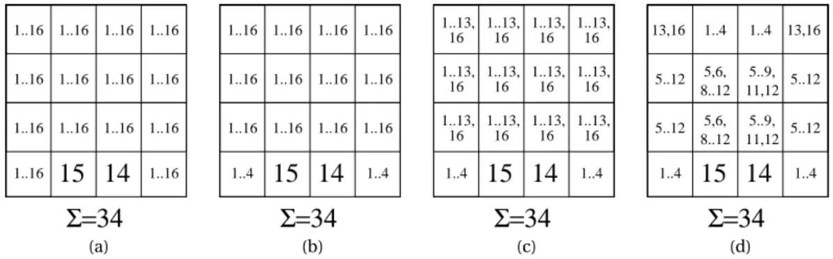
2.1. Domain taxonomy . . . 13 2.2. Partially filled magic square of order 4: without any filtering (a); where some
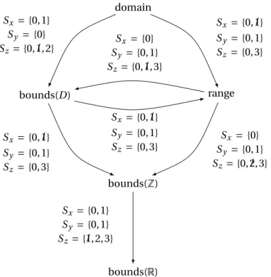
in-consistent values were filtered (b,c); with no inin-consistent values (d). . . 14 2.3. Taxonomy of constraint propagation strength. Each arrow specifies a strictly
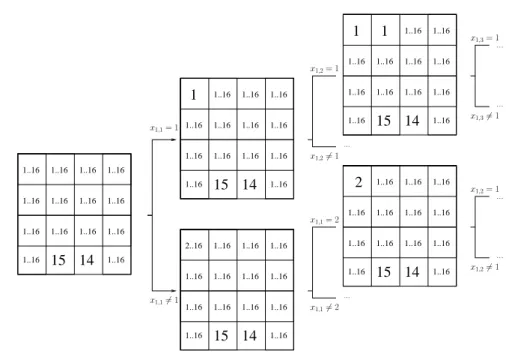
stronger thanrelation between two consistencies (see example 2.39). . . 18 2.4. Partial search tree obtained byGenerateAndTeston the magic square problem. 20 2.5. Partial search tree obtained bySOLVEon the magic square problem while
main-taining local domain consistency. . . 22
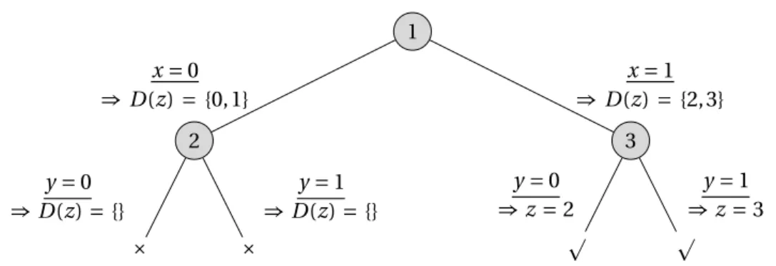
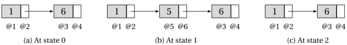
3.1. A possible search tree for the CSP described in example 3.11. Search decisions are underlined. . . 32 3.2. Contents of the stack used by the copying method for handling state. . . 32 3.3. Contents of the stack used by the trailing method for handling state. . . 33 3.4. Contents of the queue used by the recomputation method for handling state. . . 34 3.5. Reversible single-linked list. Memory addresses of the values and pointers
com-posing the data structure are shown below each cell. . . 35
4.1. Example of a CSP with variablesx1,x2,x3, and propagatorsπ1,...,π4. . . 44
4.2. Suspension list . . . 53
5.1. a) Powerset lattice for {a,b,c}, with set inclusion as partial order. b) Lattice cor-responding to the set domain [{b},{a,b,c}]. . . 60 5.2. ∆GLBx
1 and∆ LUB
x1 delta sets and associated iterators after each propagation during
the computation of fixpoint for the problem described in example 5.14. . . 69 5.3. Updating thePOSSset and storing the corresponding delta using a list splice
op-eration assuming a doubly linked list representation. . . 70
6.1. Computations involved in the composition of views described in example 6.30. . 86 6.2. Application of the view-based propagator for the composed constraint described
7.1. View model lattice. . . 99
8.1. An unbalanced expression syntax tree. The internal nodesn1...nn−1represent
operators and leafsl1...lnrepresent variables. . . 121 9.1. Number of solutions per second when enumerating all solutions of a CSP with a
given number of variables (in the xx axis), domain of size 8, and no constraints. . 144
10.1.Number of problems solved (yy axis) after a given time period (xx axis). The graphs show the results obtained for, from left to right, the graph coloring in-stances, the random inin-stances, and latin square instances. . . 158 10.2.Difference between the number of problems solved when using the LA
heuris-tic and when using the DOM+MINheuristic (yy axis) after a given time period (xx axis). The graphs show the results obtained for, from left to right, the graph coloring instances, the random instances, and latin square instances. . . 159 10.3.Number of problems solved when using several strategies (yy axis) after a given
List of Tables
4.1. Geometric mean, standard deviation, minimum and maximum of ratios of prop-agation times when solving the set of benchmarks using implementations of the models described above. . . 57
5.1. Worst-case runtime for set domain primitives when performing non-incremental propagation. . . 62 5.2. Worst-case runtime for set domain primitives when performing incremental
prop-agation. . . 70 5.3. Geometric mean, standard deviation, minimum and maximum of ratios of
run-time for solving the first set of benchmarks described above using the presented implementations of incremental propagation, compared to non-incremental prop-agation. . . 74 5.4. Geometric mean, standard deviation, minimum and maximum of ratios of
run-time for solving the second set of benchmarks (graph problems) using the vari-able delta implementation of incremental propagation, compared to propagator deltas. . . 74
7.1. Constraint propagator completeness. . . 92 7.2. Strength of the view modelmfor a set of arithmetic constraints. . . 107
8.1. Cost of accessing and updating an arbitrary expression represented by each of the described models. . . 123
9.1. Geometric mean, standard deviation, minimum and maximum of the ratios de-fined by the runtime of best performing model using views over the runtime of the best performing model using auxiliary variables, on all benchmarks. . . 140 9.2. Geometric mean, standard deviation, minimum and maximum of the ratios
de-fined by the number of fails of the best performing solver using views over the number of fails of the best performing solver using auxiliary variables, on all in-stances of each problem where the number of fails differ. . . 141 9.3. Geometric mean, standard deviation, minimum and maximum of the ratios
9.4. Geometric mean, standard deviation, minimum and maximum of the ratios de-fined by the runtime of the solver implementing the PVIEWSmodel over the
run-time of the solver implementing the CPVIEWSmodel, on all benchmarks. . . 142
9.5. Geometric mean, standard deviation, minimum and maximum of the ratios de-fined by the runtime of the CaSPER solver implementing the VARS+GLOBALmodel over the runtime of the Gecode solver implementing the VARS+GLOBALmodel, on all benchmarks. . . 143
9.6. Geometric mean, standard deviation, minimum and maximum of the ratios de-fined by the runtime of the CaSPER solver implementing the PVIEWSmodel over the runtime of the Gecode solver implementing the VARS+GLOBALmodel, on all benchmarks. . . 143
10.1.Results for finding the first solution to latin-15 with a selected strategy. . . 161
11.1.Global constraint propagators used in solvers. . . 164
11.2.Summary of features in each solver. . . 168
B.1. Number of global constraints of each kind present in each benchmark . . . 201
B.2. Propagation time (seconds) for solving each benchmark using each model (table 1/2) . . . 202
B.3. Propagation time (seconds) for solving each benchmark using each model (table 2/2) . . . 203
B.4. Social golfers: 5w-5g-4s (v=25,c/v=11.2,f=25421) . . . 204
B.5. Social golfers: 6w-5g-3s (v=30,c/v=13.6,f=1582670) . . . 204
B.6. Social golfers: 11w-11g-2s (v=121,c/v=55.4,f=10803) . . . 204
B.7. Hamming codes: 20s-15l-8d (v=42,c/v=10,f=7774) . . . 205
B.8. Hamming codes: 10s-20l-9d (v=22,c/v=5,f=59137) . . . 205
B.9. Hamming codes: 40s-15l-6d (v=82,c/v=15.1,f=27002) . . . 205
B.10.Balanced partition: 150v-70s-162m (v=212,c/v=11.7,f=48525) . . . 206
B.11.Balanced partition: 170v-80s-182m (v=242,c/v=13.4,f=54573) . . . 206
B.12.Balanced partition: 190v-90s-202m (v=272,c/v=15,f=57424) . . . 206
B.13.Metabolic pathways: g250_croes_ecoli_glyco (f=916) . . . 206
B.14.Metabolic pathways: g500_croes_ecoli_glyco (f=2865) . . . 207
B.15.Metabolic pathways: g1000_croes_scerev_heme (f=2466) . . . 207
B.16.Metabolic pathways: g1500_croes_ecoli_glyco (f=4056) . . . 207
B.17.Winner determination problem: 200 (f=1550) . . . 207
B.18.Winner determination problem: 300 (f=2924) . . . 207
B.19.Winner determination problem: 400 (f=6693) . . . 208
B.20.Winner determination problem: 500 (f=16213) . . . 208
List of Tables
B.22.Linear 20var-30val-6cons-8arity-2s (UNSAT) (S=98.14) . . . 208
B.23.Linear 40var-7val-12cons-20arity-3s (UNSAT) (S=112.29) . . . 209
B.24.Linear 40var-7val-10cons-40arity-3s (UNSAT) (S=112.29) . . . 209
B.25.NonLinear 20var-20val-10cons-4term-2fact-2s (SAT) (S=86.44) . . . 209
B.26.NonLinear 50var-10val-19cons-4term-2fact-1s (SAT) (S=166.1) . . . 210
B.27.NonLinear 50var-10val-28cons-4term-3fact-1s (UNSAT) (S=166.1) . . . 210
B.28.NonLinear 50var-5val-20cons-4term-3fact-1s (UNSAT) (S=116.1) . . . 210
B.29.NonLinear 50var-6val-26cons-4term-4fact-1s (UNSAT) (S=129.25) . . . 211
B.30.NonLinear 60var-4val-24cons-4term-4fact-5s (UNSAT) (S=120) . . . 211
B.31.Social golfers: 5week-5group-4size (S=432.19) . . . 211
B.32.Social golfers: 6week,5group,3size (S=351.62) . . . 212
B.33.Social golfers: 4week,7group,7size (S=1100.48) . . . 212
B.34.Golomb ruler: 10 (S=58.07) . . . 212
B.35.Golomb ruler: 11 (S=68.09) . . . 213
B.36.Golomb ruler: 12 (S=76.91) . . . 213
B.37.Low autocorrelation binary sequences: 22 (S=22) . . . 213
B.38.Low autocorrelation binary sequences: 24 (S=25) . . . 214
B.39.Fixed-length error correcting codes: 2-20-32-10-hamming (S=640) . . . 214
B.40.Fixed-length error correcting codes: 3-15-35-11-hamming (S=525) . . . 214
B.41.Fixed-length error correcting codes: 2-20-32-10-lee (S=640) . . . 215
B.42.Fixed-length error correcting codes: 3-15-35-10-lee (S=525) . . . 215
B.43.CPAI’08 competition results (n-ary intension constraints category) . . . 216
List of Algorithms
1. GenerateAndTest(d,C) . . . 19 2. Solve(d,C) . . . 21
3. Propagate1(d,C) . . . 26 4. Propagate2(d,P) . . . 27 5. Propagate3(d,P) . . . 29
6. PropagatePC(d,P) . . . 42 7. PropagateVC(d,V) . . . 43 8. PropagatePCEvents(d,E) . . . 47 9. PropagateVCEvents(d,E) . . . 48 10. Execute(d) . . . 49 11. Notify(e) . . . 50 12. Notify(e) . . . 51 13. Methodνi.Call() . . . 52 14. FindUb(m) . . . 100
15. SCθ(d,X,C) . . . 151 16. RSCθ(d,X,C) . . . 151 17. SReviseθ(x,d,C) . . . 152 18. SReviseInfoθ(x,d,C,INFO) . . . 153 19. Solveθ(d,C,INFO) . . . 154
Chapter 1.
Introduction
1.1. Constraint reasoning
Constraint reasoning may be introduced with a simple example. Consider the following well known combinatorial object:
Definition 1.1(Magic Square). An ordernmagic square is an×nmatrix containing the num-bers 1 ton2, where each row, column, and main diagonal equal the same sum (the magic constant).
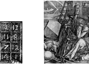
Magic squares were known to Chinese mathematicians as early as 650 BC. They were often regarded as objects with magical properties connected to diverse fields such as astronomy, mythology and music [Swaney 2000]. Figure 1.1 shows one of the earliest known squares, part of Albrecht Dürer’s engravingMelancholia.
Problems involving magic squares range from completing an empty or partially filled magic square, or counting the number of magic squares with a given order or other mathematical properties. Solving these problems presents various interesting challenges: while filling an empty magic square of odd order may be accomplished in polynomial time, completing a par-tially filled square is NP-complete, and finding the exact number of squares with some dimen-sion is #P-complete (see e.g. [Spitznagel 2010]).
The combinatorial structure inherent to this puzzle together with its simple declarative de-scription makes it a good candidate for a constraint programming solving approach. Figure 1.2 shows a constraint program which finds a magic square where the numbers 15 and 14 (the date of the engraving) are already placed as in Dürer’s original. The program embodies the following outstanding features of this technology:
Figure 1.1.: Magic square found in Albrecht Dürer’s engravingMelancholia(1514).
1 void magic ( Int n) {
2 const Int k = n*(n*n+1)/2.0;
3 Solver solver ;
4 DomVarArray<Int ,2 > square ( solver , n , n, 1 , n*n ) ; 5 solver . post ( d i s t i n c t ( square ) ) ;
6 MutVar<Int > i ( solver ) ;
7 for ( Int j = 0 ; j < n ; j ++) {
8 solver . post (sum( a l l ( i , range ( 1 ,n ) , square [ i ] [ j ] ) ) == k ) ; 9 solver . post (sum( a l l ( i , range ( 1 ,n ) , square [ j ] [ i ] ) ) == k ) ;
10 }
11 solver . post (sum( a l l ( i , range ( 1 ,n ) , square [ i ] [ i ] ) ) == k ) ; 12 solver . post (sum( a l l ( i , range ( 1 ,n ) , square [ i ] [ n−i−1])) == k ) ; 13 solver . post ( square [3][1]==15 and square [ 3 ] [ 2 ] = = 1 4 ) ;
14 i f ( solver . solve ( l a b e l ( square ) ) ) 15 cout << square << endl ;
16 }
1.2. This dissertation
Declarativeness Constraint programs are compact and highly declarative, promoting a clear separation between modeling the problem (the user’s task: lines 2-13) and solving the problem (the solver’s task: line 14). Moreover, imposing additional constraints to the problem can be done incrementally in a declarative fashion.
Efficiency Constraint programs are efficient. The above program solves the puzzle instan-taneously, and when adapted for counting is able to enumerate all the 7040 possible magic squares of order 4 in a couple of seconds.
Constraint programs explicitly or implicitly make use of a constraint solver. The constraint program of fig. 1.2 references a set of objects which are responsible for the constraint solving process. In this case, the constraint solver is implemented as a C++ library. In contrast, some constraint programs are written in a language different from the language implementing the constraint solver, in which case a conversion phase is required. We will use the term constraint solver to denominate the set of algorithms and data structures that ultimately implement the constraint programming approach.
Constraint programming embraces a rich set of techniques and modeling protocols target-ing general combinatorial problem solvtarget-ing. While our puzzle illustrates this class of prob-lems, the prominence of constraint programming arises from its application to solve real world problems in diverse areas such as scheduling, planning, computer graphics, circuit design, language processing, database systems, and biology, among many others.
Related work
Ï The magic square, Latin square, sudoku, and other related problems mostly arise as recre-ational devices, although Latin squares, a special case of a multipermutation, have found application in cryptography [Laywine and Mullen 1998].
Ï The annual conference of the field,Principles and Practice of Constraint Programming (CP), uncovers a myriad of applications of constraint programming to solve real world problems. The proceedings of its 2008’s edition features, among others, examples of CP applied to planning and scheduling [Moura et al. 2008], packing [Simonis and O’Sullivan 2008], and biology [Dotu et al. 2008].
Ï A very complete essay on all aspects of constraint programming is [Rossi et al. 2006].
1.2. This dissertation
1.2.1. Motivation
con-sider this endeavor was the lack of a constraint solver which was both competitive, extensible, open-source, and written in a popular, preferably object-oriented, programming language. We found these are necessary attributes for a constraint solver aiming to be a general constraint solving research platform.
Achieving the optimal balance between efficiency and extensibility is challenging for any large software project in general, and in particular for a constraint solver. Our hypothesis was that one does not necessarily sacrifices the other if the solver is based on a solid architecture, specifically designed with these concerns in mind.
1.2.2. Contributions
Committing ourselves to this project presented us with many interesting problems. Many of them have been solved by others, often in different ways, since practical constraint solvers have been around since the 80’s. However, until very recently the constraint programming comunity has partially disregarded implementation aspects. The architecture and design de-cisions used in most of these solvers is thus many times not fully described, discussed, or jus-tified. Therefore, for many problems we had to find our own solution given that the solutions found by others were either (a) not published, (b) jeopardized efficiency or extensibility, or (c) did not fit well with the rest of our architecture.
Presenting, explaining and evaluating all decisions behind the design of a constraint solver would be an enormous task, and perhaps not very interesting since many of these decisions condition each other. Instead, we have deliberately chosen to present what we believe are the most interesting and original ideas in our solver, hoping that they may be useful to others as well. Additionally, we also included our work on look-ahead search heuristics, which is the first application of our solver fulfilling its purpose: to be a research platform on constraint programming.
The four major contributions of this dissertation may thus be summarized as follows:
Techniques for incremental propagation We introduce a framework for integrating incremen-tal propagation in a general purpose constraint solver. The contribution is twofold: a gener-alized propagation algorithm assisting domain agnostic incremental propagation, and its ap-plication for incremental propagation of finite set constraints, showing how the framework efficiently supports domain specific models of incremental propagation.
1.2. This dissertation
Look-ahead heuristics We present a family of variable and value search heuristics based on look-ahead information, i.e. information collected while performing a limited amount of search and propagation. In particular, we describe how to integrate these heuristics with propagation algorithms achieving a specific form of consistency, namely singleton consistency, adding a negligible performance overhead to the global algorithm. We show that the resulting combi-nation compares favorably with other popular heuristics in a number of standard benchmarks.
CaSPER We developed a new constraint solver implementing the techniques discussed in this dissertation. The solver was designed with efficiency, simplicity and extensibility as primary concerns, aiming to fulfill the need of a flexible platform for research on constraint program-ming. Its flexibility and competitive performance is attested throughout this dissertation, ei-ther when used for implementing and evaluating the specific techniques discussed, but also when compared globally with other state-of-the-art solvers.
Most of the material in this dissertation has appeared on the following publications, although with a different, less uniform presentation.
Marco Correia, Pedro Barahona, and Francisco Azevedo(2005). CaSPER: A Programming Environment for Development and Integration of Constraint Solvers.Workshop on Constraint
Programming Beyond Finite Integer Domains, BeyondFD’05(proceedings).
Marco Correia and Pedro Barahona(2006). Overview of an Open Constraint Library. ERCIM
Workshop on Constraint Solving and Constraint Logic Programming, CSCLP’06(proceedings),
pp. 159–168.
Marco Correia and Pedro Barahona(2007). On the integration of singleton consistency and look-ahead heuristics. Recent Advances in Constraints, volume 3010 ofLecture Notes in Artifi-cial Intelligence, pp 62–75. Springer.
Marco Correia and Pedro Barahona(2008). On the Efficiency of Impact Based Heuristics.
Principles and Practice of Constraint Programming, CP’08(proceedings), volume 5202 of
Lec-ture Notes in Computer Science, pp. 608–612. Springer.
Ruben Duarte Viegas, Marco Correia, Pedro Barahona, and Francisco Azevedo(2008). Us-ing Indexed Finite Set Variables for Set Bounds Propagation. Ibero-American Conference on Artificial Intelligence, IBERAMIA’08, volume 5290 ofLecture Notes in Artificial Intelligence, pp. 73–82. Springer.
1.2.3. Overview
This dissertation is organized as follows.
Chapter 2 Presents the conceptual and operation models behind constraint solving and in-troduces the formalism used throughout this dissertation.
The first part covers incremental propagation, and is composed of chapters 3-5:
Chapter 3 Summarizes the major design decisions and techniques used in state-of-the-art constraint solvers, in particular its main constraint propagation algorithm, commonly used techniques for maintaining state, and other less frequently discussed, nevertheless important architectural elements. The chapter provides the necessary background for the first part of the dissertation.
Chapter 4 Describes two standard propagation models, namely variable and propagator cen-tered and discusses a set of commonly used optimizations. Shows that, when compared to variable centered algorithms, the use of a propagator centered algorithm is advantageous in a number of aspects, including performance. Introduces a new generalized propagator centered model which brings to propagator centered models a feature originally unique to variable cen-tered models - support for incremental propagation.
Chapter 5 Shows that incremental propagation can be more efficient than non-incremental propagation, in particular for constraints over set domains. Describes and compares two dis-tinct models for maintaining the information required by incremental propagators for con-straints over sets. Provides an efficient implementation of these models that takes advantage of the generic incremental propagation kernel introduced in the previous chapter.
The second part of the dissertation focuses on propagation of decomposable constraints, and is composed of chapters 6-9:
Chapter 6 Presents the formal model used for representing propagators over arbitrary decom-posable constraints, which is used extensively throughout the second part of the dissertation. Extends the notation introduced in [Tack 2009] to accommodate constraints involving an arbi-trary number of variables. Additionally, shows how sound and complete propagators may be obtained for this type of constraints.
1.2. This dissertation
Chapter 8 Details a realization of the theoretical model introduced in the previous chapters for obtaining propagators with specific type of completeness. Shows how these propagators may be efficiently compiled for arbitrary decomposable constraints. Performs a theoretical comparison of the compilation and propagation algorithms with other algorithms for prop-agating arbitrary decomposable constraints, in particular the popular method based on the introduction of auxiliary variables and propagators.
Chapter 9 Describes the implementation of the compilation and propagation algorithms for decomposable constraints discussed in the previous chapter. Performs a set of experiments for evaluating the performance of such implementations.
The third part of the dissertation aims at evaluating the CaSPER solver as a general research platform and consists of chapters 10-11:
Chapter 10 Describes a set of search heuristics which explore look-ahead information. Shows how to efficiently integrate these heuristics with strong consistency propagation algorithms. Evaluates the performance of the solver in a number of benchmarks using these and other popular search heuristics.
Chapter 2.
Constraint Programming
This chapter will introduce several important concepts used in constraint programming, and provide an overview of the two major actors of the constraint solving process, namely con-straint propagation and search. Simultaneously, it will present the notation and formal model used throughout this dissertation for describing many aspects of constraint solving.
2.1. Concepts and notation
2.1.1. Constraint Satisfaction Problems
A constraint satisfaction problem (CSP) is traditionally defined by a set of variables modeling the unknowns of the problem, a set of domains which define the possible values the variables may take, and a set of constraints that express the relations between variables. Before we for-malize CSPs, let us detail these concepts.
Definition 2.1(Assignment). An assignmentais a mapping from variables X to valuesV. A
total assignmentmaps every variable inX to some value, while apartial assignmentinvolves only a subset ofX. We represent an assignment using a set of expressions of the formx7−→v, meaning that variablex∈Xtakes valuev∈V.
Definition 2.2(Constraint). A constraintcdescribes a set of (partial) assignments specifying the possible assignments to a set of variables in the problem. We may represent a constraint by extension by providing the full set of allowed assignments, or by intension in which case we will write the constraint expression in square brackets. A partial assignmentais consistent with some constraintcifabelongs to the set of assignments allowed byc.
Example 2.3(Assignment,Constraint). The assignment a1 ={x17−→1,x27−→3} assigns 1 to
variablex1and 3 to variablex2. The assignmenta2={x17−→2,x27−→3} assigns 2 to variablex1
and 3 to variablex2. The constraintc={{x17−→2,x27−→1},{x17−→1}} may also be represented
asc=[(x1=2∧x2=1)∨x1=1]. The assignmenta1is consistent with the constraintc, while
In theory, variables and constraints are sufficient to model a CSP, since constraints may be used to specify all the domains of the variables in the problem. However, most textbook defi-nitions of CSPs explicitly specify an initial set of values for the variables in the problem, which will be refered to asvariable domains.
Definition 2.4(Variable domain). A variable domaindD⊆Drepresents the set of allowed
val-ues for some variable. Common variable domains aredZfor integer variables,d2Zfor integer
set variables, anddRfor real-valued variables. WhenDis omitted we assumedZ.
We may now define constraint satisfaction problems.
Definition 2.5(CSP). A Constraint Satisfaction Problem is a triple〈X,D,C〉whereXis a finite set of variables, D is a finite set of variable domains, andC is a finite set of constraints. We will denote by D(x) the domain of some variable x∈X. Similarly, we will refer to the set of constraints involving some variable x ∈X asC(x). The set of variables in some constraint
c∈Cmay be selected withX(c).
The task of solving a CSP consists of finding a solution, i.e. one total assignment which is consistent with all constraints in the problem, or proving that no such assignment exists.
Example 2.6(Magic square as a CSP). We can easily formalize the problem of filling an-order magic square, introduced in the previous section. The CSP consists of n2 integer variables, one for each cell. Each variablexi,j ∈X represents the unknown figure corresponding to the cell at position¡i,j¢in the square, where 1≤i ≤n, 1≤j ≤n, and have the initial domain
D¡xi,j ¢
=©1,...,n2ª. This corresponds to line 4 in the program of figure 1.2 on page 2. Let
k =n¡n2+1¢/2 denote the magic constant. The CSP’s constraint setC is composed of the following constraints:
^
1≤i,j,k,l≤n:i6=k∨j6=l £
xi,j6=xk,l ¤
all cells take distinct values (line 5)
^
1≤i≤n X
1≤j≤n £
xi,j=k ¤
the sum of cells in the same row equalsk(line 8)
^
1≤i≤n X
1≤j≤n £
xj,i=k ¤
the sum of cells in the same column equalsk(line 9)
P
1≤i≤n £
xi,i=k ¤ P
1≤i≤n £
xi,n−i=k
¤ the sum of cells in the main diagonals equalsk(lines 11,12)
2.1.2. Tuples and tuple sets
2.1. Concepts and notation
Definition 2.7(Tuple). Ann-tuple is a sequence ofnelements, denoted by angle brackets. We make no restriction on the type of elements in a tuple, but tuples of integers will be most often used. Tuples will be refered by using bold lowercase letters, optionally denoting the number of elements in superscript.
Definition 2.8(Element projection). We will writetj to refer to thej-th element of tuplet, in which case we consider tuples as 1-based arrays. Similarly, we extend the notation to allow multiple selection, writingtJ=
tj ®
j∈Jto specify the tuple of elements at positions given by set J.
Example 2.9(Tuple, Element projection). Consideringt3= 〈2,3,1〉, a 3-tuple, we havet2= 〈3〉
(or simplyt2=3), andt{1,3}= 〈2,1〉.
Definition 2.10(Tuple set). A tuple setSn⊆Zn is a set ofn-tuples, also referred to as table. When needed, we will refer to the size of the tuple set, the number of tuples, as|Sn|.
Definition 2.11(Tuple projection). Let projj(Sn)=©tj:t∈Sn ª
the projection operator. We generalize the operator for projections over a set of indexes, projJ(Sn)=©tJ:t∈Sn
ª .
Example 2.12(Tuple set, Tuple projection). S3={〈1,2,3〉,〈3,1,2〉} is a 3-tuple set, with size ¯
¯S3¯¯=2. Then proj2¡S3¢={〈2〉,〈1〉} and proj{2,3}¡S3¢={〈2,3〉,〈1,2〉}.
Definition 2.13(Assignments as tuples). Throughout this dissertation we will implicitely use tuples to represent assignments. A given assignment {x17→v1,...,xn7→vn} may be represented by ann-tupletn= 〈v1,...,vn〉. If an assignmentti is a partial assignment, i.e. covers only a subsetX′ofX, then the sizeiof the tuple equals the number of variables inX′, that isi=¯¯X′¯¯, in which case the setX′will be made explicit.
Definition 2.14(Constraints as tuple sets). We may also represent constraints as tuple sets. The notation con(c) specifies the set of tuples corresponding to the partial assignments al-lowed by the constraint. It is assumed that the set of partial assignments alal-lowed by the con-straint affects the same set of variables. This does not restrict the expressiveness of the notation since any partial assignment may be extended to cover more variables by taking the Cartesian product of the allowed values in the domains of the remaining variables.
Example 2.15. LetD(x1)={1,2}, andD(x2)={1,2,3}. The assignmenta={x17−→1,x27−→3}
may be represented asa= 〈1,3〉. Letcbe a constraint defined asc={{x17−→2,x27−→1},{x17−→1}}.
Then con(c)={〈2,1〉,〈1,1〉,〈1,2〉,〈1,3〉}. The fact that the assignmentais consistent with the constraintcis equivalent to the expressiona∈con(c).
2.1.3. Domain approximations
Definition 2.16(Cartesian approximation). The Cartesian approximationVSnWδof a tuple set
Sn⊆Znis the smallest Cartesian product which containsSn, that is:
VSnWδ=proj1¡Sn¢×...×projn¡Sn¢
Definition 2.17(Box approximation). Given an ordered setS⊆D, let conv(S) be the convex
set ofS, i.e.
convD(S) = {z∈D: min(S)≤z≤max(S)}
The box approximation VSnWβ(D) of a tuple setSn ⊆Dn is the smallestn-dimensional box
containingSn, that is:
VSnWβ(D)=convD
¡
proj1¡Sn¢¢×...×convD
¡
projn¡Sn¢¢
We will be referring to integer and real box approximations exclusively, i.e. V·Wβ(Z)orV
·Wβ(R).
WheneverDis omitted it will be assumed thatD=Z.
We introduce one more operator, the identity operator, which will be used mostly for sim-plifying notation:
Definition 2.18(Identity approximation). The identity operatorV·Wϕtransforms a tuple set in itself, i.e.VSnWϕ=Sn.
LetSn,Sn1,Sn2⊆Znbe arbitraryn-tuple sets andΦ∈©ϕ,δ,βª. We note the following
proper-ties of these operators:
Property 2.19(Idempotence). TheV·WΦ
operator is idempotent, i.e.VSnWΦ=VVSnWΦWΦ.
Property 2.20(Monotonicity). The V·WΦ
operator is monotonic, i.e. Sn1 ⊆Sn2 =⇒ VSn1WΦ
⊆
VS2nWΦ.
Property 2.21. TheV·WΦ
operator is closed under intersection, i.e.VSn1WΦ∩VS2nWΦ=VVS1nWΦ∩
VS2nWΦWΦ.
These domain approximation operators will be used extensively to specify particular types of tuple sets calleddomains.
2.1.4. Domains
2.1. Concepts and notation
−domains
−domains
−domains
Figure 2.1.: Domain taxonomy
Domains will be used for multiple purposes. First we note that, by definition, any tuple set is aϕ-domain. For any CSP〈X,D,C〉we can also observe the following: The setD of variable domains is aδ-domain capturing the initial set of variable assignments. For any constraint
c∈C, con(c) is a domain specifying the possible assignments toX(c), and the conjunction of all constraints con(Vc∈Cc) in the problem is also a domain specifying the solutions to the problem.
The following concepts define a partial order on domains.
Definition 2.23. A domainSn1 ⊆Znisstrongerthan a domainSn2 ⊆Zn(or equivalentlySn2 is
weakerthanSn1), if and only ifSn1 ⊆Sn2. Sn1 isstrictly strongerthanSn2 (or equivalentlySn2 is
strictly weakerthanSn1) if and only ifSn1⊂Sn2.
The following lemma shows how the previously defined approximations are ordered for a given tuple set.
Lemma 2.24. Let Sn⊆Znbe an arbitrary tuple set. Then, Sn=VSnWϕ⊆VSnWδ⊆VSnWβ
Note that this contrasts with the relation between all possibleΦ-domains withΦ∈©ϕ,δ,βª,
as depicted in figure 2.1.
Related work
15 14
Σ=34
1..16 1..16 1..16 1..16 1..16 1..16 1..16 1..16 1..16 1..16 1..16 1..16 1..16 1..16 (a)15 14
Σ=34
1..16 1..16 1..16 1..16 1..16 1..16 1..16 1..16 1..16 1..16 1..16 1..16 1..4 1..4 (b) 1..13, 16 1..13, 16 1..13, 16 1..13, 16 1..13, 16 1..13, 16 1..13, 16 1..13,161..13, 16 1..13, 16 1..13, 16 1..13, 16
15 14
1..4 1..4Σ=34
(c) 5,6, 8..12 5..9, 11,12 5,6, 8..12 5..9, 11,1215 14
1..4 1..4Σ=34
1..4 5..12 5..12 5..12 5..12 1..4 13,16 13,16 (d)Figure 2.2.: Partially filled magic square of order 4: without any filtering (a); where some incon-sistent values were filtered (b,c); with no inconincon-sistent values (d).
Ï The Cartesian approximation was defined in [Ball et al. 2003], while box approximation is defined in [Benhamou 1995]. Domain approximations in the context of constraint program-ming were further refined by Benhamou [1996], and Maher [2002], and reconciled with the classical notions of consistency in [Tack 2009].
2.2. Operational model
Solving constraint satisfaction problems involves two main ingredients: propagation and search. Propagation infers sets of assignments which are not solutions to the problem and excludes them from the current domain. Search finds assignments which are possible within the current domain. The solving process consists of interleaving the execution of these two procedures, exploring the problem search space exhaustively until a solution is found.
2.2.1. Propagation
Let us revisit the magic square problem introduced earlier:
Example 2.25(Magic Square filtering). Imagine Dürer’s task of finding a magic square with the figures 14 and 15 already placed. He probably began by writing an empty square, where all values are possible in all cells except in those which are already assigned (similar to the square of fig. 2.2 a). Soon he must have realized that some values were impossible in some cells, namely in the two inferior corners, which must add to 5 (fig. 2.2 b), and in all remaining cells, which cannot take 14 nor 15 since they are already placed (fig. 2.2 c).
2.2. Operational model
further and removed all inconsistent values from the initial problem, ending with the partial magic square shown in fig. 2.2 (d).
The amount of filtering performed on a CSP is related to a property known asconsistency. Before we give the classical definition of consistency regarding CSPs, let us first focus on con-sistencies of an arbitraryδ-domain with respect to a single constraint, which basically tell us how well the domain approximates the constraint.
Definition 2.26(Domain consistency). Aδ-domainSn is domain consistent for a constraint
c∈Cif and only ifSn⊆Vcon(c)∩VSnWδWδ.
Definition 2.27(Bounds(Z) consistency). Aδ-domainSn is bounds(Z) consistent for a con-straintc∈Cif and only ifSn⊆Vcon(c)∩VSnWβWβ.
Definition 2.28(Bounds(R) consistency). Aδ-domainSn is bounds(R) consistent for a con-straintc∈Cif and only ifSn⊆Vcon(cR)∩VSnWβ(R)Wβ(R).
Definition 2.29(Bounds(D) consistency). Aδ-domainSnis bounds(D) consistent for a con-straintc∈Cif and only ifSn⊆Vcon(c)∩VSnWδWβ.
Definition 2.30(Range consistency). Aδ-domainSnis range consistent for a constraintc∈C
if and only ifSn⊆Vcon(c)∩VSnWβWδ.
The above concepts define different consistencies by requiring that all members of the do-main lie within some neighborhood of the constraint. Intuitively, for a given consistency the inner approximation operatorV·Wtell us which solutions to the constraint are taken into con-sideration, while the outerV·Wdefines the set of non-solutions which are acceptable.
Example 2.31(Consistency). Consider the sum constraintc(corresponding to the bottom row of the magic square in fig. 2.2), and the tuple setS4={1,2,4}×{15}×{14}×{1,2,3,4}. The set of solutions that domain and bounds(D) consistency must approximate is con(c)∩VSnWδ=
{〈1,15,14,4〉,〈2,15,14,3〉,〈4,15,14,1〉}. SinceVcon(c)∩VSnWδWδ={1,2,4}×{15}×{14}×{1,3,4}⊂ S4, then S4 is not domain consistent to constraintc. Similarly, since Vcon(c)∩VSnWδWβ =
{1,2,3,4}×{15}×{14}×{1,2,3,4}⊃S4, thenS4is bounds(D) consistent to constraintc.
The notion of consistency applies naturally to a given set of constraints and domain of a CSP, in which case it may be referred to aslocal consistencyorglobal consistencyof the constraint network as explained below.
Definition 2.33(Global consistency). A CSP〈X,D,C〉is globally domain consistent (respec-tively globally bounds(Z), bounds(R), bounds(D), or range consistent), if and only ifD is do-main consistent (respectively bounds(Z), bounds(R), bounds(D), or range consistent) for the constraintVc∈Cc.
Example 2.34(Consistency of a CSP). The CSP corresponding to the magic square of figure 2.2 (b) is locally bounds(Z) and bounds(D) consistent, but not domain nor range consistent. The square shown in (c) is locally domain consistent (and consequently also locally bounds(Z), bounds(R), bounds(D), and range consistent). The square shown in (d) is globally domain consistent.
The computational cost of achieving local and global consistency on a given CSP depends on the constraint network structure, on the semantics of the constraints involved, and on the size of the domains. Achieving global consistency is usually intractable except for CSPs with a very specific network structure, but polynomial time algorithms exist that achieve local consistency for a number of important constraints. Perhaps because it is easier to reason with independent constraints rather than with their conjunction, constraint propagation has been traditionally implemented in modular, independent components called propagators, which achieve some form of local consistency on specific constraints.
Definition 2.35(Propagator). A propagator (or filter) implementing a constraintc ∈C is a functionπc:℘(Zn)→℘(Zn) which is contracting, i.e.πc(Sn)⊆Snfor any tuple setSn⊆Zn. A propagator is sound if and only if it never removes tuples which are allowed by the associated constraint, i.e. con(c)∩Sn⊆πc(Sn) for any tuple setSn⊆Zn.
Traditionally, propagators were also required to be monotonic, i.e. πc¡Sn1¢⊆πc¡S2n¢ifSn1 ⊆ Sn2, and idempotent, i.e. πc(πc(Sn))=πc(Sn), however these additional restrictions are not mandatory in modern constraint solvers, as shown in Tack [2009]. Throughout this disserta-tion we will consider propagators to be monotonic and will not make any assumpdisserta-tion about its idempotency unless explicitely stated. Moreover, we will use the following notation con-cerning idempotency.
Definition 2.36(Idempotent propagator). Letπc be a propagator for a constraintc∈C. Let π⋆c represent the iterated functionπ
⋆
c =πc◦...◦πc such thatπc ¡
π⋆c(x) ¢
=π⋆c(x). Propagator πc is an idempotent propagator forSnif and only ifπc(Sn)=π⋆c (Sn). In such case we also say thatπc(Sn) is a fixpoint forπc, or equivalently thatπcis at fixpoint forπc(Sn). Propagatorπcis an idempotent propagator if and only ifπc(Sn) is a fixpoint forπcfor anySn⊆Zn. Finally, we remark that we always haveπc(Sn)⊂SnunlessSnis a fixpoint forπc. This is a consequence of πcbeing deterministic, and is independent of the idempotency ofπc.
2.2. Operational model
for example the identity function. Useful propagators are complete with respect to some do-main, which translates in achieving some consistency on the constraint associated with the propagator. According with our previous definitions of consistency, we now enumerate the corresponding completeness guarantees provided by propagators.
Definition 2.37(Domain completeness). A propagator πc implementing constraintc∈C is domain complete if and only ifπ⋆c(Sn) is domain consistent for the constraintc, for anyδ -domainSn. In such case we say the propagator achieves domain consistency for the constraint
c.
Definition 2.38(Bounds completeness). A propagatorπc implementing constraintc ∈C is bounds(Z) (respectively bounds(R), bounds(D), or range) complete if and only if π⋆c(Sn) is bounds(Z) (respectively bounds(R), bounds(D), or range) consistent for the constraintc, for anyδ-domainSn.
Example 2.39(Propagator completeness taxonomy). Domain completeness and the different types of bounds completeness described above are ordered as shown in figure 2.3. Each arrow reflects astrictly stronger thanrelation between two completeness classes.
Additionally, we labeled arrows with a tuple setSfor which the propagator at the start of the arrow is able to prune more values (marked as striked out) than the propagator at the end of the arrow. For this, we considered a propagatorπc for the constraintc=
£
2x+3y=z¤and a tuple setS=Sx×Sy×Sz. For example, when applied to a domainS={〈0,1〉,〈0〉,〈0,1,2〉}, a domain complete propagator is able to prune tuples〈0,0,1〉and〈1,0,1〉whereas a bounds(D) cannot. Note that bounds(D) complete and range complete propagators are incomparable.
Related work
Ï Historically, the notion of consistency was associated with CSPs involving extensional con-straints. Mackworth [1977a] presented an algorithm for achieving domain consistency on CSPs involving binary extensional constraints, and later generalized for non-binary con-straints [Mackworth 1977b]. The algorithm was referred to as arc consistency in the case of binary relations, and generalized arc consistency for n-ary relations. Although the term is still commonly used, we will use domain consistency throughout this dissertation. The presented bounds consistency definitions are described in more detail in chapter 3 of [Rossi et al. 2006]. The formalization of domain and bounds consistency and completeness using domain approximations is due to Tack [2009], which is in turn based on [Maher 2002] and [Benhamou 1996].
domain
bounds(D)
bounds(Z)
bounds(R)
range
Sx ={0,1} Sy ={0} Sz ={0,1/,2}
Sx ={0,1/} Sy ={0,1} Sz ={0,3}
Sx ={0,1/} Sy ={0,1} Sz ={0,3}
Sx ={0} Sy ={0,1} Sz ={0,2/,3}
Sx ={0,1} Sy ={0,1} Sz ={1/,2,3}
Sx = {0} Sy ={0,1} Sz ={0,1/,3}
Sx ={0,1/} Sy ={0,1} Sz ={0,3}
2.2. Operational model
FunctionGenerateAndTest(d,C)
Input: A domaindand a set of constraintsC
Output: A subsetS⊆dsatisfying all constraints inC, i.e.S⊆con(c) :∀c∈C
ifd= ;then 1
return;
2
if|d| =1∧ ∀c∈C,d⊆con(c)then 3
return{d}
4
〈d1,d2〉 ←Branch(d)
5
returnGenerateAndTest(d1,C)∪GenerateAndTest(d2,C)
6
generalization is intentional, since it will be used in part II. However, we kept the classi-cal notions of consistency and propagation completeness associated to Cartesian products. Applying the same generalization there would make comparing to existing propagation al-gorithms more complex.
Ï A line of research in constraint programming is devoted to identifying tractable constraint network structures, where global consistency may be achieved in polynomial time. See for example chapter 7 of [Rossi et al. 2006]. For a complete characterization of tractable CSPs for 2-element and 3-element domains see [Schaefer 1978; Bulatov 2006].
Ï A number of polynomial algorithms have been identified that achieve domain or bounds consistency in a number of useful constraints. A notable example is the constraint that enforces all variables to take distinct values (used in the magic square example) for which an algorithm exists that achieves domain consistency in timeO¡n2.5¢by Régin [1994], another achieving bounds(Z) on timeO¡nlogn¢by Puget [1998], and a range complete propagator which runs in timeO¡n2¢by Leconte [1996]. Algorithms achieving bounds(D) consistency are rarely found in practice.
Ï Consistencies stronger than domain consistency have been proposed, namely path consis-tency [Montanari 1974], andk-consistency [Freuder 1978]. These consistencies approxi-mate constraints using domains stronger thanδ-domains, whose representation requires exponential space, and are disregarded in most constraint solvers.
2.2.2. Search
Generate and test is a brute force method that generates all possible combinations of values and then selects those that satisfy all constraints in the problem. The method is easily imple-mented using recursion (functionGenerateAndTest).
15 14
1..16 1..16 1..16
1..16 1..16 1..16 1..16 1..16 1..16 1..16 1..16 1..16 1..16 1..16 15 14
2..16 1..16 1..16
1..16 1..16 1..16 1..16 1..16 1..16 1..16 1..16 1..16 1..16 1..16 14 1..16 1..16 1..16 1..16 1..16 1..16 1..16 1..16 1..16 1..16 1..16 1..16 1..16 15 1 14 1..16 1..16 1..16 1..16 1..16 1..16 1..16 1..16 1..16 1..16 1..16 1..16 15 1 1 15 14 1..16 1..16 1..16 1..16 1..16 1..16 1..16 1..16 1..16 1..16 1..16 1..16 1..16 2
x1,3= 1
x1,36= 1
x1,2= 1
x1,26= 1 ...
...
...
...
x1,26= 1
x1,16= 2
x1,1= 2
x1,2= 1
...
...
x1,16= 1
x1,1= 1
Figure 2.4.: Partial search tree obtained byGenerateAndTeston the magic square problem.
and satisfy all constraints in the problem. Otherwise, line 5 calls a functionBranchthat splits the domaindin two smaller domainsd1,d2, such thatd=d1∪d2andd1∩d2= ;, and line 6
calls the function recursively on each of these domains.
Figure 2.4 shows a trace, orsearch tree, of the algorithm applied to the magic square prob-lem. The leftmost square represents the initial domain, and the direct children of each square are the domains resulting from theBranchfunction.
TheGenerateAndTestalgorithm may generate an exponential number of domains that do
not contain any solution. An example is the topmost square in fig. 2.4 that corresponds to a non-singleton domain which does not contain any solutions since the same value is used in the first two cells of the first row. An improved version of this algorithm is given by function
Solve.
The difference is the inclusion of a call to thePropagatefunction, which filters inconsis-tent values from the input domain, as discussed in the previous section. The search tree of the
Solvealgorithm now depends on the consistency achieved by constraint propagation. For
ex-ample, ifPropagateenforces local domain consistency on this problem, we obtain the partial search tree shown in figure 2.5, where each square corresponds to the domain obtained after propagation (line 1). Note that all the upper children which cannot lead to any solution are immediately rejected, hence the algorithm avoids exploring an exponential number of nodes.
2.2. Operational model
FunctionSolve(d,C)
Input: A domaindand a set of constraintsC
Output: A subsetS⊆dsatisfying all constraints inC, i.e.S⊆con(c) :∀c∈C
d←Propagate(d,C)
1
ifd= ;then 2
return;
3
if|d| =1∧ ∀c∈C,d⊆con(c)then 4
return{d}
5
〈d1,d2〉 ←Branch(d)
6
returnSolve(d1,C)∪Solve(d2,C)
7
enough time it will find a solution or prove that no solution exists, which is in fact one of the most appealing aspects of the constraint programming approach. Additionally, it is also space efficient since only one child of each node must be in memory at all times, and the depth of the search tree is bounded by the number of variables and values in their domains. Unfortunately, the time efficiency of this algorithm greatly depends on the way the search tree is explored, i.e. on the order in which the child nodes of a given node are visited (line 7). A number of heuristics have been proposed that try to direct search towards the solution, with some success for many combinatorial problems. However, the algorithm will, in the worst case, explore the full search tree before finding the solution or proving that it does not exist.
Although other complete search algorithms exist, they are essentially variations of theSolve
algorithm. Therefore, in this dissertation we will assume that search is performed using this algorithm.
Related work
Ï TheSolvealgorithm is also known asbacktracking. Other popular complete algorithms
that may be used with constraint propagation are backmarking,forward checking,
back-jumping, among others [Dechter 2003].
1..13, 16 1..13, 16 1..13, 16 1..13, 16 1..13, 16 1..13, 16 1..13, 16 1..13, 16 1..13, 16 1..13, 16 1..13, 16 1..13, 16 14 15 1..4 1..4 1..13, 16 1..13, 16 1..13, 16 1..13, 16 1..13, 16 1..13, 16 1..13, 16 1..13, 16 1..13, 16 1..13, 16 1..13, 16 2..13, 16 14 15 1..4 1..4 1..12, 16 1..12, 16 1..12, 16 1..12, 16 1..12, 16 1..12, 16 1..12, 16 1..12, 16 1..12, 16 1..12, 16 1..12, 16 14 15 1..4 1..4 13 14 15 1..4 1..4
16 1..13 1..13 4..13
1..13 1..13 4..13 4..13
1..13 4..13 1..13 4..13
x1,16= 1
x1,1= 1
x1,1= 13
x1,16= 13
x1,16= 2
x1,1= 3
x1,16= 3
x1,1= 2
...
...
...
Figure 2.5.: Partial search tree obtained by SOLVEon the magic square problem while main-taining local domain consistency.
of value to enumerate, and is often obtained by integrating some knowledge about the struc-ture of the problem [Geelen 1992].
2.3. Summary
Part I.
Chapter 3.
Architecture of a Constraint Solver
This chapter will describe a number of important techniques and decisions behind the design and implementation of a modern constraint solver. It will focus on two main components: a propagation kernel implementing generalized constraint propagation (§3.1), and the state manager, responsible for maintaining the state of all elements of a constraint solver synchro-nized with the search procedure (§3.2). Additionally, this chapter will present other important structural resources of constraint solvers, such as the support for domain specific reasoning, global constraints, and language interfaces (§3.3). Whenever possible, we will provide point-ers to state-of-the-art constraint solvpoint-ers which advertise the use of a particular method. In this same spirit, this chapter will also perform a global overview of CaSPER, the constraint solver used for implementing and evaluating all the techniques described in this dissertation.
3.1. Propagation kernel
The propagation kernel forms the core of a constraint solver. Because propagation takes the largest share of time spent on solving a given problem, designing a propagation kernel involves decisions that affect the global performance of a constraint solver.
3.1.1. Propagation loop
Most constraint solvers do not maintain a specific type of consistency in particular, but in-stead achieve an hybrid form of local consistency. They associate one or more propagators with specific strengths with each constraint of the problem, and combine their propagation by repeatedly executing propagators until a fixpoint is achieved. The existence of a fixpoint, hence the termination of the algorithm, is guaranteed since propagators are contracting and domains are finite, as we have observed in the previous chapter. A very simple implementation of this algorithm is given by functionPropagate1.