Policy uncertainty and informational monopolies: the case of monetary policy

. .

I

_{I ,.}

FUNDAÇÃO

4fI""

Getulio Vargas

EPGE

Escola de Pós-Graduação em Economia

Seminários de Pesquisa Econômica

11

(J a

parte)

"POLlCY Ul\TCERTAll\TTY Al\TD

Il\TFOBlVIATIOl\TAT. lVIOl\TOPOLlES:

TBIí: CASE OF lVIOl\TETARY

POLlCY"

J

RODOLFO

E.

MANUELLI

OI

•

Preliminary and Incomplete Comments Welcome

Policy Uncertainty and Informational Monopolies:

The Case of Monetary Policy

by Larry E. Jones and Rodolfo E. Manuelli I

This version: July 28, 1996 First version: April 1, 1995

I MEDS, Kellogg School, Northwestem University and Department of Economics, University of

li

..

•

1. Introduction

There are at least two important reasons why volatile governrnent policy can affect real allocations. First, volatility can result in a confusion on the part of individual agents between real and policy shocks. This creates a costly signal extraction problem for the agents in the economy. Second, even in the absence of any real shocks to the system variable policy can create situations in which agents on opposite sides oftrades can be asymmetrically informed about the state of policy. In this paper, we concentrate on this second aspect of policy volatility and model the possibility of informational monopolies which arise due to the strategic use of these informational differences.

Although this problem could arise in any setting in which governrnent' s actions are uncertain, a natural environrnent to study these issues is where there is uncertainty about monetary policy. (The high leveI ofmonetary policy uncertainty and its relationship to the average leveI of inflation is well documented, see Barro (1995).) Thus, this research continues an important line of inquiry into the mechanisms through which uncertain monetary policy has real effects begun with the seminal work ofLucas (1972). In that paper, Lucas first showed that asymmetric information about the realization of the money supply can result in monetary shocks affecting output since agents cannot perfectly distinguish real from monetary shocks. Since that initial work on the subject, a variety of papers have studied different environrnents and different mechanisms through which uncertain monetary policies have real effects (see, for example, Lucas (1987), (1989), Lucas and Woodford (1993), Eden (1994), Benabou and Gertner (1993), and Jovanovic and Veda (1996)). A common feature in this work is that asymmetric information about monetary policy plays a leading role. This paper contributes to this literature by offering a new perspective on the roles played by two elements: the strategic use of information and the resulting incentives for costly information gathering activities. This is one possible explanation for the observation that the size of the financial intermediary sector is larger in countries with high and variable inflation (cf. Aiyagari and Eckstein (1993)).

The model that we analyze is a simple static bargaining model in which buyers and sellers are potentially differentially informed. When a buyer and a seller are matched they bargain over the terms of the transfer of one unit of an indivisible good. If the parties agree to transfer the good, the buyer makes a money payment to the seller. Residual cash balances are used to buy units of a divisible good. We assume that the realization ofthe money supply follows a commoniy known stochastic law and choose units ofthe divisible good so that its price equals the money supply.

•

,

•

neutra!. That is, changes in the money supply process that have the form of a positive constant times the "old" money supply process give rise to the same real allocation. Further, it can be shown that if either both parties are informed or both parties are uninformed, there are no real effects ofvariability in the money supply. (This result is a special case ofthat given in Chwe, that if information is symmetric, monetary policy has no real effects.)

This environrnent produces some interesting results both when the information structure is taken as given, and in the case in which individual agents determine whether they will be informed about the realization of the money supply.

Consider first the case of a buyer who is perfectly informed and a seller who is uninformed. We show that, depending on parameters, it is possible that a "lemons problem" (cf. Akerloff (1970)) in money can arise. That is, since both parties to the agreement share a common, but uncertain, value ofthe good, 'money,' the seller, when setting his price must take into account the fact that the only time the buyer wiIl accept the offer is when the value of money is low (i.e., the money supply is large). This uncertainty about the value of cash has a non-monotonic effect on prices: for smalllevels of variability of the money supply, increases in variance decrease prices, while for high levels the opposite holds. When volatility is high enough, this last effect dominates trade causing the probability of exchange to decrease to zero even though it is common knowledge among the parties that the buyer values the good more highly than the seIler. This welfare loss (i.e., the probability of trade being less than one) is simply a problem of an informational. monopoly induced by the policy uncertainty. To see this we show that ifthere are two buyers, both informed, the optimal mechanism from the seIler's point ofview has a probability oftrade equal to one independent ofthe variability in the money supply processo (Also, as noted above, ifthe parties are symmetricaIly informed, there is no welfare 10ss.). Finally, even for parameter values in which the probability oftrade is one independent ofthe variance ofthe money supply, changes in volatility can have redistributive effects.

This is, we believe, a feature common to asymmetries of information induced by policy volatility: Since both parties share an interest in the outcome of the policy variable, the informational problem is of the common value, rather than the independent value formo It is because of this form of informational asymmetry that there can be both welfare losses from private information and common knowledge of gains to trade.

CF

or general overviews of these two cases, see Myerson (1985) and Kennan and Wilson (1993).)

Even though our emphasis is on the real effects of different monetary regimes, this model shares many of the features of other monetary models that rely on asymmetric information and

,

•

realization ofthe money supply).

This characterization depends critically on our assumption that the buyer is informed and the seller is not. We study the other altematives and show that when both parties share the same information structure the probability of trade is one; while when buyers are uninformed and sellers are informed high variability ofthe money supply results in a probability oftrade less than one, and in contractionary effects ofunforeseen increases in the money suppIy. This raises the question of the determination of the information structure in this setting.

We next consider the case in which agents choose their information leveis. We study a two stage game in which buyers and sellers can choose to leam the realization of the money supply at some cost. In the second stage they are randomly paired. Our previous description of the effects of policy uncertainty on the equilibrium of a given match, suggests that the payoffs to becoming informed are low at both Iow and high leveis of uncertainty. At low leveIs of variability the expected value of any given amount of money is dose to its certainty value. Information is not very valuabIe. At the other end, high variance results in high prices and low probability of a transaction. In this case, information is not very valuable either. This intuition carries over to the equilibrium in which all agents choose their information structure as long as the parties values for the indivisible good are not too far apart. We show that for both low and high variances alI individuais choose to be uninformed. For intermediate values ofthe variance ofthe money supply, the unique symmetric equilibrium is in mixed strategies with varying fractions ofbuyers and sellers being informed. In this region the inefficiency of equilibrium is due to two factors: first, trade occurs with probability less than one; second, real resources are used to acquire socialIy useless information.

In the case in which buyers' and selIers' valuations are far apart, policy uncertainty has a smaller impact on the probability oftrade (which is one over a much larger region). However, the artificially created value of information induces agents to spend resources on acquiring

information and, even for high leveis of policy variability, the equilibrium is inefficient. Since the good is traded with high probability, information does not lose its value when the variance of the money supply increases. Thus, unlike the case of similar valuations, there is an equilibrium in which a positive fraction of both buyers and sellers are informed for alI values of the variance of the money supply exceeding some criticallevel. In this case the inefficiency is mostly associated with the resources devoted to acquiring information.

In both of these cases, our modeI implies that the cross sectional distribution of prices for the same good (across stores or matches) is not degenerate because different sellers will be

In our model, this dispersion is driven just by informational asymmetries and hence is independent of firms' costs, search costs and the costs of changing prices. Thus, our model provides yet another mechanism through which monetary policy can result in price dispersion.

In addition to its implications on prices, the model makes predictions about the distribution of informed and uninformed agents, and shows that --due to the strategic interaction-- these are not monotonic in our measure of the variability of monetary policy. The model does not support the view that higher variance makes information more valuable and, hence, more people should be

I

informed. The reason for this is that the value of information depends on the policy in place as

welI as the actions of other agents. In this sense, the fraction of "other" agents that is informed is an important as the variability of the money supply in determining the decision to beco me inf-ormed on the part of any single individual.

<lO

•

The papers that are closest to this one are CaselIa and Feinstein (1990) and Chwe (1995). Casse lIa and Feinstein consider a dynamic bargaining situation in which there is no asymmetric information and inflation acts as a taxo In their particular formulation, inflation reduces the effective discount rate and this, in turn, affects the outcome of the bargaining game. The key result in their paper is that producers wilI charge different prices depending on the age (or wealth since they are perfectly correlated) ofthe buyers that are in the store. Chwe (1995) considers a model in which buyers and selIers are asymmetrically informed about both the value of money and their private valuations of the indivisible good. He shows that there wilI be no welfare loss associated with private information about money as long as the value of money is common knowledge or agents share the same priors and information partition. He also shows that when individuaIs have different priors_monetary uncertainty can increase the sum of expected utilities. Chwe also studies the effect of an exogenously changing fraction of informed traders and shows that the resulting equilibrium displays Phillips curve like features. Our work emphasizes the point that it is the informational monopoly that is important and that its degree of importance depends on how variable monetary policy is.

In section 2 we present the basic model for fixed information structures. Section 3 explores the impact of changes in policy uncertainty upon the equilibrium when information structures are not allowed to change. In sections 4 and 5 we concentrate on the case in which the differences in the valuation of the indivisible good between buyers and sellers is small. In section 4 we study a two stage game. In the first stage individuals choose their information structure, and in the second stage they are randomly matched. We show that an equilibrium exists and we partially

characterize it. Section 5 contains most of our comparative statics results. In section 6 we discuss the case of large differences in valuation, while section 7 offers some preliminary conclusions.

2. The Basic Model and Equilibrium with Symmetric Information

•

I

•

'.

followed by an accept/reject decision by the buyer. We analyze the equilibrium when the two parties are symmetrically informed/uninformed and show that monetary policy is neutral in this case.

Both the buyer and the seller derive utility from two goods: an indivisible good which gives utility vb to the buyer (if purchased) and vS to the seller, and another which we call general

consumption. We assume that utility is additive and given by,

where xb, restricted to be either O or 1, represents consumption of the indivisible good and c is the'level of general consumption. We assume that subsequent units ofthe indivisible good do not yield any utility. We treat the seller symmetrically and assume that his utility function is given by,

At this point we take the valuations of both buyers and seIlers as given, and assume that vb:>vs. This assumption implies that trading the indivisible good is always the ex post efficient outcome.

The buyer has an initial endowment of money mb . If the seIler announces the price p and the buyer purchases one unit of the indivisible good, the buyer's consumption of the general consumption good is cb = (mb-p)/M. Here we have imposed that the price ofthe consumption good is equal to the money supply M. This simply follows from our choice of units of the divisible good, and can be rationalized by imposing a cash-in-advance constraint on divisible consumption that opens after the value of M becomes common knowledge. Let the seller's endowment be ms. Then, if he sells the indivisible good, his leveI of general consumption is (ffis+P)/M. Without loss of generality assume that mb=ÃM, while ffis=(l-Ã)M, where O:s::Ã:s:: l.

With these conventions it is possible to write the indirect utility function (with some abuse of notation) for each ofthe parties given that they know M and the price p has been announced by the seller as,

We restrict the buyer's announced price to be measurable function ofhis information. We take M to be a random variable, and assume that its distribution is common knowledge .

Since the buyer knows this and knows the value of M, the equilibrium has the seller charging the price p(M) = vbM. The good is exchanged with probability one and the seller extracts all of the surplus from the buyer. We summarize the equilibrium in the following proposition.

Proposition 2.1. In the case ofan informed buyer meeting an informed seller, (1,1), the

equilibrium outcome is characterized by,

(i) The indivisible good will be traded with probability one. [q(l,I)= 1]

I (ii) The price announced by the seIler is p(M)= vbM. (iii) The expected utilities of the two parties are,

WS(I,I) = l-À

+

vb,

ｾＨｉＬｉＩ＠ = À.

(iv) Monetary policy is neutral. The allocation and (both ex ante and ex post) utilities oftwo agents do not depend on the distribution for M.

Note: Throughout, we wiIl denote the 'information state' by a pair, (Y,Z) where Y and Z E

{U,I},

Y

denotes the informational status ofthe buyer and

Z

is that ofthe seller. Of course, U means that the agent is uninformed and I means that the agent is informed.

Next, consider first the case of an uninformed buyer meeting an uninformed seller. Here, since the seller does not know the vaIue ofM, the announced price does not depend on M. Thus, the expected utility of the buyer if the price is p is his unconditionaI expected utility. If he purchases the good utility is,

while the expected utility of not buying the good is À. Thus, the rule the buyers uses is: buy if the price is less than or equaI to vblE(M·I). It is clear that --ifthe seller decides to sell at all-- he will always charge the price p = vblE(M-I). (RecaII that given the information structure the seller is restricted to making price offers that do not depend on M.) Thus,

(2.3) p(M)= vblE(M-1).

Whether the seller will choose to sell the indivisible good depends on the comparison of its utility in the two cases. It is easy to check that the seller will choose to sell if and only ifthe price it can get is greater than or equal to vSIE(M-1). Since this is less than p(M) trade will occur with probability one at the monopoly price p = vblE(M-1_{). To simplify notation in what follows, define}

f.! to be E(M-1_).

We summarize this discussion in the following proposition.

Proposition 2.2. In the case of an uninformed buyer meeting an uninformed seller, (D,U), the

---(i) The indivisible good is traded with probability one. [q(U,U)=I] (ii) The price announced by the seller is p(M)= vb_/Il.

(iii) The expected utilities of the two parties are, WS(U,U) = l-À

+

vb,

ｾＨｕＬｕＩ］￀Ｎ＠

(iv) Monetary policy is neutral. The allocation and (ex ante, expected) utilities oftwo agents are the sarne as ifthe random variable 11M was equal to its mean value with probability one. Thus, they do not depend on the distribution for M. Ex post welfare does depend on

I the realization of M, however.

..

Note that, for this infonnational structure, prices depend on the mean ofthe inverse ofthe money supply and --as before-- are independent ofrelative wealth. Payoffs (and income) are

independent ofmonetary policy, and dependjust on initial wealth and monopoly power.

The neutrality results presented here (i.e., Proposition 2.1 (iv) and Proposition 2.2 (iv» are reminiscent Chwe's (1995) common knowledge results. There, it is shown that whenever both parties share the sarne prior beliefs (which is the only case we consider) and their infonnation partitions are the sarne, money is neutral.

3 The Case with Asymmetric Information

In this section, we generalize the model presented above to consider cases of asymmetric

infonnation. We consider both the case of an uninfonned seller facing an infonned buyer as well as an infonned seller facing an uninfonned buyer. We show that in these two cases, money is not neutral in general. The character of the equilibrium depends both on which party is infonned and the distribution goveming the money supply, M. There are some general properties, however. In general, the probability oftrade is strictly less than one (as long as there is 'enough variance') and hence equilibrium is inefficient. The one exception to this is when there is no variability at all in the money supply. In this case, the good is exchanged with probability one and the outcome is efficient (no matter which party is infonned). The model does generate a Phillip's curve, a non-trivial, equilibrium reIationship between the leveI of M and the probability of trade of the good, but the direction of this relationship depends on which party is the infonned one.

3.1 Uninformed Sellers and Informed Buyers

Consider the case in which an uninfonned selIer meets an infonned buyer. We assume that the infonnation structure is common knowIedge: the seller and the buyer both know who is informed and who is uninformed. We study the anaIogue ofthe garne analyzed in section 2 in which the seller has alI the monopoIy power. More precisely, we consider a timing ofmoves in which the seller announces a price, and the buyer can either accept or reject. We do not allow any

counteroffers.

following the arguments in Myerson (1985) and Samuelson (1984), it can be shown that this game implements the outcome of the mechanism that maximizes the utility of the seller given incentive compatibility and individual rationality on the part ofthe buyer when the buyer is informed and the seller is not:

Proposition 3. J. J Assume that distribution of M has compact support with a density which is

everywhere positive and that the buyer is informed and the seller is noto Then, the outcome of the bargaining game is identical to that of the mechanism that maximizes the utility of the seller

1 given incentive compatibility and individual rationality ofthe buyer.

•

Proo!" The proof is contained in Appendix A.

To analyze the model in this case, consider first the buyer's decision. Since he knows the

realization of M, given the price p, the optimal decision is to buy the indivisible good if and only if,

vb

₊

_{Ã-p/M > Ã, or equivalently, v}b

₊

_{(ÃM-p)/M > ÃMIM.}

Thus, the buyer's optimal decision rule is,

buy if (3.1.1)

l do not buy if p>Mvb •

The seller knows this rule (this is the sense in which it extracts alI the surplus) but --in this case--does not know the realization of M. Since the seller is restricted to announcing prices that are independent ofthe realization ofM (this is where the measurability restriction is binding), the seller chooses p to maximize,

(3.1.2) _{V '(p) =}

_{flX(P<M.'p -}

_{Á +}

ｾＩ＠

_{+( 1 -}

ｘＨｐ＼ｍＮｾＩ｛ｶ＠

_{'+ 1 - Á+F}

_M

where F M is the cdf of the random variable M. Let p* denote the solution to this maximization

problem.

With this investment in notation, it is possible to give two types of neutrality results for this model. First, notice that ifthe distribution ofM is a point mass at some value m*, it follows immediately that the seller will announce the price p=m*vb_{• Given this, the buyer will always}

A second type of neutrality result holds even in cases in which there may be welfare losses from inflation. This is that the equilibrium outcome of the model is identical for any linear

transformation of the money supply processo That is, inspection of the decision rule for the buyer above shows that for the random variable «M with «>0, the optimal decision rule for the buyer has a reservation price which is « times as high as with the random variable M. Given this feature, it follows immediately from (3.1.2) that the optimal price from the seller's point ofview when the money supply is given by «M is to choose a price equal to «p* where p* is the optimal price under the original distribution of M. It follows from this that the probability of trade as

I well as the realized leveIs of welfare are invariant to this type of change in the distribution of M (although equilibrium nominal prices are affected). For this class of experiments money is neutral. Note that adding a constant to the random variable M does not give a neutrality result. We summarize these results in the following proposition:

•

Proposition 3.1.2:

(i) If the distribution of M places probability one on the value m *, the equilibrium has the seller charging the price p = m*vb. The indivisible good is exchanged with probability

one and the outcome is efficient.

(ii) Both the probability oftrade and the realized leveis ofutility are invariant to positive multiples in the probability distribution ofthe money supply. The equilibrium price under a money supply rule given by M' = «M with «>0, is «p* where p* is the

equilibrium price under the original money supply rule M.

It tums out that it is convenient to describe (3.1.2) in terms of the distribution of the inverse of the money supply. Thus, let F be the cdf ofthe random variable 11M, and assume that it has a

density f. The random variable M is assumed bounded, ｏ＼ｭｌｾｍｾｭｵ＼ｯｯＮ＠ Note that an equivalent description of the optimal decision rule by the buyer is that he buys the indivisible good if and only if llM<vb/p. Thus, the seller's indirect utility over prices is given by,

(3.1.3)

v b,p

V b

V S(p)

=

1 -À +p

f

xf(x)dx +(1 -F(-;»V s.

11m U

First, note that if the seller charges the price p=mLVb the buyer will accept the offer with probability one. Thus, the seller will always choose prices such that ｰｾｭｌｶ｢Ｎ＠ At the other extreme, any price exceeding mUvb will result in a zero probability oftrade.

In order to characterize equilibrium behavior in the model, we make a special assumption about the distribution, F:

I

•

supply has a uniform distribution on [Jl-k,Jl+ k], where Os:k < Jl,

11M - U [Jl-k,Jl+ k].

Note that given this speeifieation mL_{=I/[Jl+k], and m}U_=lI[Jl-k].

To simplify notation, it is use fuI to express VS as a fraetion ofvb_. More speeifieally, define e by:

Then, e measures how far apart the values of the buyer and selIer are. This, in turn, measures the potential gains from trade between the two parties. Thus, if e= 1, vS:O, and the spread between yS

and yb is maximal and the potential gains from trade are vb while if e = 0, VS:yb and there are no

gains from trade.

We need one last bit ofnotation before deseribing the equilibrium behavior in this environrnent. Let k(Jl,e) be defined (for ･ｳＺｾＩ＠ by

_ [1 -(1 -2e)I/2]

ｫＨｾＬ･Ｉ＠ -ｾ＠ .

[1 +(1 -2e)1I2]

As it turns out, the qualitative behavior of the equilibrium depends on whether k is smaller or larger than k(Jl,e) as welI as the size of e itself.

The Equilibrium of lhe Bargaining Game

The selIer maximizes (3.1.3) given its expeetations about the realization ofthe money supply. Optimal behavior on the part of the buyer is eompletely summarized by the "purehasing rule" (3.1.1).

We are now ready to deseribe the equilibrium ofthe bargaining game.

Proposition 3.1.3. Let p(Jl,k,e) be the solution to the selIer's problem (maximization of (3.1.3)

subject to bounds constraints) and let q(Jl,k,e) denote the resulting probability ofthe object being traded. Then,

i) If e<1I2 the equilibrium is eharaeterized by,

a) b)

Ifks:k(Jl,e), p(Jl,k,e)=pL and q(Jl,k,e)=l,

Ifk>k(Jl,e), but k<Jl, p=V'(1-2eylí_{l(Jl-k) and q(Jl,k,e)=(Jl-k)[(l-2e)"V: - 1]/2k <1.}

Proof

The seller's objective function is continuous but not differentiable in the interior of

8t.

The interval [O,pL] is easy to handle. In this region, the good will be sold with probability one, and the function yS(P) is increasing in p. It follows that the seller will never announce a price less than pL. Let pU be the lowest price such that the buyer does not purchase the good for any realization I ofM. In our setting pU is given by vb/(j..l-k). For prices ｰｾｰｵＬ＠ the function YS(p) isjust

l-À+(1-e)vb, a constant. It is immediate to check that in the interval (PL,pU) function is strictly concave if e<1I2, linear if e=1/2, and strictly convex if e> 112. We are now ready to discuss the various cases.

•

i) [e<1I2]. In this case the objective function is concave in the relevant interval ＨｐｾｰｌＩＮ＠ The first order condition for the seller's maximization problem with the additional requirements that ｰｾｰｌ＠

(with Lagrange multiplier y) is,

or,

g

xf(x)dx - (Vb/p)2 f(vb/p)e + y = 0,

where z= vb/p and y=l/mu. Using the specific form for f(x) we get,

Altematively, this condition is,

Depending on the size of j..l-k, it is possible that even when p=pL, the Lagrange multiplier is positive. Define kL as the lowest value of k such that (*) is satisfied with p=pL and y=O. Thus, kL must satisfy,

or,

,..-.---

ＭｾＭＭＭＭＭＭＭＭ

kL = k(Jl,e).

From the definition ofk(Jl,e) it follows that kL is unique. We now show that for k>kL the unique p that solves the first order condition assuming y=O is strictly greater than pL. To see this impose y=O and solve for p. The solution is,

I To check that p>pL we need to check that,

•

which corresponds to,

(l-2ef' > (Jl-k)/(Jl+k), or equivalently, k> k(Jl,e).

The candidate solution automatically satisfies p<pu=vb/(Jl-k). Finally, note that the probability of trade is given by q(Jl,k,e)=Pr(p < Mvb) = Pr(l1M < vb/p). Using the expression for p(Jl,k,e) and the form for F shows that

q(Jl,k,e) = (Jl-k)[(1-2ef' -1]/2k

as desired.

ii) We first consider the case e=1/2. It is easy to check that the derivative ofVs(P) is negative and given by -(Jl-kl/2k on (PL,pU). It follows that the optimal policy is to charge pL, which results in a sale with probability one.

If e> 1/2 the function VS(P) is convex on (pL,pU). It is c1ear that the solution must be a comer solution: the optimal price is either pL or pU. The respective utilities are,

For the seller to weakly prefer pU over pL it must be the case that,

Jl/(Jl+k) ｾ＠ (l-e),

or --given the restrictions on e in this case-- that,

This, however, leads to a contradiction since the right si de ofthe previous inequality is bounded above by Yz. It follows that the seller will always choose pL, and the indivisible good is sold with

probability one.

•

This simple model delivers the standard result in many fixed (or predetermined) (see Lucas (1989) and Lucas and Woodford (1993) for examples with explicit micro foundations) price models: an expansionary monetary policy reduces the real cost of goods for sal e and it increases

i output. In our case, the result is rather extreme due to the indivisibility of the good; for low

values ofthe money supply there is no trade (and output is low), while for high values output is efficient.

•

As Proposition 3.1.3 shows, the qualitative behavior of the equilibrium depends on whether e is less or greater than one. In the remainder ofthis subsection, as well as in sections 4 and 5, we concentrate on the case e<1I2. The other case --large differences in valuation-- is discussed in section 6 and Appendix D.

Changing the volatility of M

Next, we will discuss the consequences of changing the volatility ofthe money supply upon the equilibrium when the buyer is informed, but the seller is not. Proposition 3.1.3 gives us a partial, but incomplete accounting for what happens when uncertainty about policy is increased. There, holding ｾ＠ fixed, as k is increased, the probability oftrade decreases toward zero. Notice here however that we are simultaneously changing both the average value ofM (it goes to infinity) and its variance (we are holding ｾ］＠ E(I/M) fixed). The problem is that changes in k holding ｾ＠

constant are not equivalent to increases in the variance of M, holding its mean constant. For this reason, we will be interested in simultaneously changing k and ｾ＠ so that E(M) is fixed. In this way, we can isolate the effect of changing the volatility of policy without changing its average value. Because of this, it is useful to summarize some properties of the family of distributions that we are working with.

Let the mean ofM be m*, m* = E(M). Then it follows that,

m*

=

｛ｬｮＨｾＫｫＩＭｬｮＨｾＭｫＩ｝ＯＲｫＮ＠

Thus, we can find for each k, the value ｯｦｾＬ＠ denoted ｾＨｫＩ＠ that satisfies this expression for a

given value ofm*. It is easy to check that,

ｲＭＭＭＭＭＭＭＭＭＭＭＭＭＭＭＭＭＭＭＭＭＭＭＭＭＭＭＭＭＭＭＭＭＭＭＭＭｾＭＭＭＭＭｾＭＭ

--

---F(m;m* ,k) = e2m-k/(e2m-k_l) - 1/(2mk).

It is straightforward to calculate the variance of M given (Il(k),k). It is,

There are two properties ofthis family of distributions that are worth emphasizing. First, for any given mean, m*, limk __ ｡ｾＨｫＬｭＪＩ］ｏｑＬ＠ and ｬｩｭｫ｟ｯ｡ｾＨｫＬｭＪＩ］ｏＬ＠ and ｡ｾＨｫＬｭＪＩ＠ is a monotone

I increasing function ofk. Thus, it is appropriate to index monetary policies by k, with higher k's (holding m* constant) corresponding to higher variance --but constant mean-- economies. FinaIly, it can be shown that increasing k with Il = Il(k) is a mean preserving spread on the distribution of M.

•

In section 3.1 we described the criticaI value k(ll,e), which played a criticaI role in determining the efficiency of an aIlocation. This was defined for a given vaIue of the mean of the inverse of the money supply, Il. Since we are interested in changes in the variance of the money suppIy holding its mean (m*) constant, it is necessary to describe the criticaI value ofk that corresponds to the threshold effect associated with k(ll,e). To this end, let kj be the uni que value ofk that satisfies,

A simple caIculation shows that kj=ln[(1-2e)"V,]/2m*.

As described in Proposition 3.1.3, the quaIitative nature ofthe solution depends on how far apart the valuation of the buyer and the seIler are. In particular, if e<1I2, for ｫｾｫｪＬ＠ the probability of trade is one while for k>kj it is strictly less than one. For that reason it wiIl be useful to

separately describe the impact of changing the variability for the different cases. We start with the situation in which the sellers' and buyers' valuations are not too far apart (VS>vb/2, or e<1I2). We study the case ･ｾ＠ ｾ＠ at the end.

From now on, to simplify notation, we wiIl ignore the dependence of the equilibrium variabIes on e and m*. In the conclusion we brief1y discuss the impact of changing them .

The Impact ofVariability on Prices

From Proposition 3.1.3 it follows that the equilibrium price charged by an uninformed seller when faced with an informed buyer is,

(3.1.4) p(I,U,k) = vbm* max{(e2m-k_l)/2m*ke2m-k, (1-2e)"" (e2m-k_-l)/2m*k}.

l

•

(3.1.5)

where,

Direct calculations show that ｾｬＨｫＩ＠ _{is continuous, decreasing and differentiable, and limk_o} ｾｬＨｫＩ］＠ 1, limk __ ｾｬＨｫＩ］＠ O. ｾＲＨｫＩ＠ is a differentiable and increasing function, and it satisfies lirnl.;_o

ｾＲＨｫＩ］ＨＱＮＲ･ｙ［ＧＬ＠ and limk __ ｾＲＨｫＩ］＠ 00. Moreover, the uni que value ofk that satisfies ｾＱＨｫＩ］ｾＲＨｫＩ＠ is

kj. Figure 1 displays candidate ｾｩ＠ functions . From (3.1.5), it follows that as the variance of the money supply increases there is a region in which prices decrease. However, once the variance·· as indexed by k-- gets past the value ｫｾＬ＠ Additional increases result in higher prices. Thus, the model predicts that in this case prices are a V -shaped function of the variance of the money supply. To understand this somewhat puzzling response of equilibrium prices to changes in the volatility ofthe money supply we consider the two regions defined by kt separately. Consider first the region of decreasing prices. In this region ··in which trade occurs with probability one--an increase in the varione--ance of the money supply forces the seller to lower prices to guarone--antee a sale, so that even in the lowest realization of the money supply the buyer finds advantageous to purchase the indivisible good. Thus, in this region, an increase in variance reduces the seller's monopoly position: uncertainty about the value that buyers put on the object and the desire to sell results in lower prices. Of course, lowering the price reduces consumption of the divisible good on the part ofthe seller. At some point this decrease in consumption is sufficiently high that the seller decides to charge slightly higher prices and face the possibility of trading with probability less than one. Thus, in this second region ··to the right ofkt in Figure 1--increases in the variance are accompanied by price increases and --as we will show shortly·- reductions in the transaction volume. Thus, we summarize this discussion in the following resulto

Proposition 3.1.4. Let e<1I2. Then the equilibrium price announced by an uninfonned seller who

meets an infonned buyer ··p(l,U,k)-- is a V shaped function ofk. It decreases for ｫｾｫｴＬ＠ and it increases for ｫｾｫｾＮ＠ Moreover, it equals

v>m*

when k is zero, and it converges to infinity as k goes to infinity.

In the spirit ofBenabou and Gertner (1993), it is possible to interpret the ratio ofp(I,U,k) and VS

as a measure of markup. As in Benabou and Gertner, the model predicts that changes in the variability of inflation (or real shocks in their setting) can either increase or decrease markups. In their setting, the key element is the size of search costs: if search costs are high, higher

uncertainty reduces search and increases prices. If search costs are low the opposite happens. In this model, the emphasis is shifted to the magnitude of the uncertainty, and its interaction with infonnational monopolies: for low levels of variability markups decrease as the value of

i

•

increases prices --the value ofthe informational monopoly decreases.

The Effect upon the Probability ofTrade

As described in Proposition 3.1.3 the probability of trade depends on the size of the variance of the money supply. As before, we study increases in k holding E(M)=m* constant. From

Proposition 3.1.3 it follows that for k in the interval [O,ktl the probability oftrade is one. In the region k>kt the probability oftrade is given by,

q(I,U,k)= Pr[llM<vb_/p].

Given our assumptions that the distribution of 11M, is U[ J.l(k)-k, J.l(k)+k], a straightforward

calculation shows that the probability of trade is,

(3.1.6) q(I,U,k)= 'i1 + ç(k),

where,

(3.1.7)

It is easy to check that ç(kt) = 'i1, lim,, __ ç(k)=-'i1, and that ç(k) is decreasing in k. We summarize these results in the following proposition.

Proposition 3.1.5. Let e<1I2. Denote by q(I,U,k) the probability that the indivisible good is

traded when an informed buyer is matched with an uninformed seller. Then, q(I,U,k) =1 for k

ｾｫｴＬ＠ and O<q(I,U,k)<1 for k>kt. Further, q(I,U,k) is decreasing in k and lirn,, __ q(I,U,k)=O.

Thus, when the variability of the money supply is large relative to the mean, the probability of trade converges to zero. In this case, the high variance of the money supply decreases the expected real value of money balances obtained by the seller. Thus, the relative valuation of the indivisible good in terms of the consumption good decreases. In this case, the seller is willing to part with the good on1y ifhe can get enough consumption in returno To accomplish this, the announced price converges to infinity (see Proposition 3.1.4), but this drives the probability of trade to zero.

The Welfare Effects ofVariable 1nflation

í

•

(3.1.8a)

For the region k >kj, the appropriate expression is,

(3.1.8b) WS(I,U ,k) = l-À +(vb_{/2( e}2m_{*k_1 ))[( 1-2eYY'-(1-2e)"»]+ [1-q(I,U,k)](1-e)vb,}

where q(l,U,k) is given by (3.1.6). Similarly, it is possible to calculate the expected utility ofthe buyer. Direct ca1culations show that in the region ｫｾｫｪＬ＠ the expected payoff to the buyer is,

(3.1.9a)

while in the region k >kj, expected utility is,

(3.1.9b)

There are two interesting features. First, in the region ｫｾｫｪＬ＠ the utility ofthe seller decreases as k

increases, while the utility of the buyer increases. The reason for this is --as described before--the incentives that sellers have to lower before--their prices in order to secure a sale, in a region in which selling strictly dominates. (In this region, the probability oftrade q(I,U,k) equals one.) Thus, in this region, increases in the coefficient of variation of the money supply process result in a redistribution ofincome from sellers to buyers by reducing the former's monopoly power.

In the region k >kj the situation is more complexo Each of the twO welfare functions involve the term

as well as a term containing the probability of trade. The interpretation of this term is simple. It

gives the value to the seller of transferring the good --conditional on a sale occurring. This term enters positively in the sellers expected utility and negatively in the buyers utility. In addition, each ofthe two parties derives utility from consuming the indivisible good. It is easy to check that (vb/2(e2m_{*k-l))[(1-2e)"Y'-(1-2ef')] is decreasing in k. Thus, as k increases the seller's expected}

surplus --even conditional on selling the good-- decreases. On the other hand, the value of not selling increases, as the probability oftrade decreases. The opposite holds for the buyer.

What happens to total welfare? Note that in this worId of linear utility functions, welfare is equivalent to expected income measured in units of the divisible good. Let aggregate welfare (or expected income) be given by ｗ］ｗｳＫｾＮ＠ It is straightforward to calculate that in the region k

ｾｫｪ＠ expected income is given by,

(3.1.10a) W(I,U,k)= 1 +vb_•

Note that this is maximal, the outcome here is ex post efficient. In the region k >kj, expected

income is,

(3.1.10b) W(I,U,k)= 1 +vb[q(I,U,k)

+

(l-e)(l-q(I,U,k))].

It follows that changes in k do not affect aggregate income in the region k ｾｫｴＬ＠ but they have redistributive consequences. On the other hand, in the region k >kt, increases in k decrease the probability of trade which, in our setting, implies inefficient outcomes. Throughout this region, real money balances are equal to one (when deflating by the price of consumption which we make equal to M), thus conventional calculations of the welfare loss associated with inflation --the area under --the demand curve-- would show no impacto Finally, --the difference between --the ex-post efficient leveI of aggregate income --1 +vb __ and the expected leveI of income as given by (3.1.1Ob) is a measure ofthe expected loss from inflation. This difference is (vb-vS)(l-q(I,U,k)), which is just the "premium" that buyers put on the indivisible good times the probability of not trading. Thus, as k increases and q(I,U,k) converges to O, the size ofthe expected weIfare (and income) loss goes to vb_vs• We summarize the results in the following proposition.

Proposition 3.1.6. Let e<1I2. Let Wj(I,U,k) denote the expected welfare (and expected income)

ofagentj,j=b,s; and let W(I,U,k) be given by Wb(I,U,k)+ws(I,U,k). Then,

i) WS(I,U,k) is decreasing for all values ofk.

ii) Wh(l,U,k) is increasing for k ｾｫｴＬ＠ and decreasing for k ｾｫｴＮ＠

iii) W(I,U,k) is constant and equal to its maximal value 1 +vb for k ｾｫｴＮ＠ For k ｾｫｴＬ＠ W(I,U,k) is given by l+vb[q(l,U,k) + (l-e)(l-q(I,U,k))] which is a decreasing function ofk which converges to 1 +vb(l-e) as k goes to infinity.

3.2

Asymmetric Information: Informed Sellers and Uninformed Buyers

Finally, we study the bargaining problem between an uninformed buyer and an informed seller, (U,I). In this case the seller knows M and can announce prices which are contingent on M. More preciseIy, we will analyze sequential equilibria ofthe game in which seller's are first informed about the value ofM, second, sellers announce a price and finally, buyers, having seen the price, but not M, decide whether or not to buy the object. A sequential equilibrium is then a choice of price by the seller for every outcome of M, p(M), an acceptlreject rule for the buyer given the price (but not M), X(P)= O or 1, and a set of beliefs about the true state of nature for the buyer given that the seller has offered the price p(M). Of course, X(P) must maximize the buyer' s utility given his beliefs and the price rule, p(M), must (for each M) maximize the sellers utility. Finally, the beIiefs ofthe buyer must be credible.

---

-probability of trade are invariant to money supply processes that are positive multiples of each other. Prices simply change by the magnitude ofthe positive multiple.

To analyze the model, first consider the problem of a buyer. Since we wiIl only be interested in pure strategy equilibria, a buyer's strategy can equally weIl be summarized by an 'acceptance set.' Accordingly, let A be the set ofprices for which the buyer will accept and trade wiIl occur. For simplicity, we will assume that the buyer can only choose among A's which contain their supremum. This is a restriction on the strategy space ofthe buyer. Note further that given any acceptance set, A, the only relevant price from this set is its supremum, sup A, since if the seIler wants to seIl the object to the buyer given what he knows about M, it is always in his interest to charge the maximal acceptable price. Ifhe doesn't want to seIl to the buyer, he can charge any price above sup A, but pu is a natural candidate. Given this, we can equivalently represent the problem ofthe buyer as choosing a reservation price, which we wiIl denote by pro

To characterize equilibrium in this setting, we will first treat pr parametrically and impose rationality on the part ofthe buyer below.

Given a level ofpr, we can characterize the optimal behavior ofthe seller. Ifthe seIler chooses the price pr, he sells the object and hence receives utility l-À +prlM, while ifhe charges any price higher than pr, he does not seIl the object and hence receives utility l-À +V'. Thus, he wiIl charge

the price pr if and only if ｍｾｭｩｮＨｭｕＬ＠ pr /v5

) == M*. If, on the other hand, M>M*, he will charge

some price higher than pro Without loss of generality, we will assume that he charges the highest possible price, pu, in this case.

This description of the optimal behavior of the seller given any reservation price rule determines the beliefs ofthe buyer using Bayes Rule. Ifthe buyer sees the price pr, the conditional

distribution on 11M given p=pr is uniform on the interval [11M*, ｾＫｫ｝Ｌ＠ while ifthe buyer sees the price pu, the conditional distribution on 11M given p--pu is uniform on the interval ｛ｾＭｫＬｬｬｍＪ｝Ｎ＠

As is standard in these models, beliefs are not pinned down for any other values of p without making further assumptions.

Given these restrictions on beliefs, we wiIl now derive the restrictions on buyers behavior that results from optimal decision making on his parto First, the utility received by the buyer ifhe buys and the price is pr is given by:

M' r r

( l

1 1

U

=

À +

f

[V -.L] dF I r

=

À + V -

L

-

+ - .

b M Mp b 2 M* L

L m

m

On the other hand, if he does not buy, his utility is À. Thus, the restrictions imposed by

..

It is straightforward to check that these strategies (with the price ofthe seIler equal to pU

whenever M>M*) do in fact constitute an equilibriurn as long as pr ｾ＠ min (ml vb _{(I+e), mU Vs ).}

Notice that min (ml vb _{(1 +e), mU}

Vs ) :::: ml vb (I +e) if and only ｩｦｫｾ＠ e Il, and min (ml vb (1 +e),

mU VS

):::: mU VS if and only ifk ｾ＠ e J..l. Thus, ifk ｾ＠ e J..l, there are equilibria ofthis type with pr up

to mU VS• The relevance ofthis is that ifpr = mU vS, the probability oftrade is equal to one and the

outcome is efficient.

On the other hand, ifpr ｾ＠ mU vs, note that this implies a probability oftrade equal to one given optímal behavior on the seIler's part and, optimality on the buyer's part reduces to pr ｾ＠ vb _J..l.

These two (i.e., pr ｾ＠ mU VS and pr ｾ＠ vb Il) are mutually consistent if and only if k ｾ＠ e Il.

Among these equilibria, we wiIl concentrate on the one that maximizes the utility of the seIler.

An altemative selection criteria would be to choose the equilibria that maximize the probability of trade. When k ｾ＠ e Il our selected equilibriurn is one of many that results in a probability of trade equal to one. When k> e J..l, our selected mechanism is the only one that makes the probability of trade maximal. Thus, there are no conflicts between these two. altemative criteria. More preciseIy, our criterion seIects the equilibriurn in which pr is at its maximal leveI. This is given by pr = vb _{J..l when k ｾ＠ e J..l and pr = ml v}b _{(I +e) when k > e Il. Since we are interested in}

studying the limits to efficiency we wilI only study this is equilibriurn.

In this equilibriurn, when k > e Il, trade occurs whenever ml ｾ＠ M ｾ＠ M* = ml( 1 +e )/( 1- e). Thus, the probability oftrade is given by:

p(

m L:$;M:$;m

dI

+e»)

=p(

(1 -e) :$; 11M

ｾ＠

11m LJ

= p(

(Il +k) (1 -e) :$; 11M:$; Il +k)

=

e(1l +k).

(1 -e) m l(1 +e) (1 +e) (1 +e)k

When k-oo with 1l=Il(k), it foIlows that this probability oftrade converges to 2 e/(I +e). Note

that this is strictly less than one (and strictly positive) whenever e < 1 (e >0). In the case that k

ｾ＠ e Il, this maximurn probability of trade is given by one. Since Il and k are not independent, it is convenient to describe the two regions in terms of a cutoff levei of k. Let ｫｾ＠ be the leveI of k such that Il(k)=ek. It is easy to check that,

ｫｾ］＠ ln[(1 +e)/(1-e)]/2m*.

It also foIlows that k ｾ＠ e J..l, if and only if k ｾ＠ ｫｾ［＠ and k > e Il, if and only if k > ｫｾＮ＠ We summarize this discussion in the following proposition:

i

equilibrium outcome is characterized by the foIlowing:

(i)

(ii)

If k :5: ｫｾＬ＠ there are a continuum of equilibria indexed by the buyer's reservation price, pr

where pr :5: vb/Il(k). These equilibria have a probability oftrade q(U,I,k) equal to one for mU_vs_{:5: pr :5: vb/Il(k). The equilibrium welfare ofthe agents (in the equilibrium that}

maximizes the welfare of the seIler) is given by:

Wh(U,I,k)

=

À, and, WS(U,I,k) = l-À + vb.

If k > ｫｾＬ＠ there are a continuum of equilibria indexed by the buyer' s reservation price, pr

where pr:5: mL _{vb/(l-e). The indivisible good wiIl be traded with probability q(U,I,k) =}

[e(1+e)][2e2m_"k/(e2m_{"k-1)] < 1. Trade occurs when M :5: m}L _{(l+e)/(l-e), i.e., when M is}

low. The equilibrium welfare ofthe agents (in the equilibrium that maximizes the welfare of the seIler) is given by:

Wb(U,I,k) = À, and,

WS(U,I,k) = l-À + vb [1- e + e q(U,I,k)].

(iii) As k-oo, the maximum probability oftrade converges to 2 e/(l +e).

Here, since the seIler has a monopoly on both market power (by virtue of moving first in the bargaining game), and the information, the buyer is pushed to his reservation utility for alI values ofk. Note that in this informational setting, the Phillip's curve goes the opposite way from the previous case. That is, here trade occurs when M is small. Finally, note that the equilibrium price in this setting does not depend on M, even though it could (i.e., the seller knows M).

4. Endogenous Information Structures

So far we have taken the information structure of the buyer-seller pairs as given. However, as the discussion in the previous section show there are policies (high k policies) for which the private gains from being informed are potentially very large. A natural extension of the analysis is to allow for the endogenous choice ofthe information structure. To that effect we study a two stage game. In the first stage individuals choose whether to become informed or not. This decision is made simultaneously by all players (buyers and sellers). In the second stage --given the

•

in information strategies that has as its payoffs the expected utilities that were calculated in the previous section. The notion of equilibrium that we use is Nash equilibrium.

We assume that the cost ofbecoming informed is given by c (measured in units ofthe divisible consumption good). This cost of acquiring information can be interpreted broadly as

encompassing private time and expenditure costs which can be affected by the govemment. As an example, secrecy mIes associated with the meetings ofthe FOMe have helped create a sizable industry ofFed watchers who try to estimate --given the fragmentary information available-- the Fed's actual policy. Ifthe Fed plainly announced in unequivocal terms its intentions and policies it is possible to imagine that this industry would greatly shrink. This is an example in which c would correspond to the cost ofpurchasing information from Fed watchers. Altematively, many accounts of hyperinflations emphasize that individuaIs spend a great deal of time trying to determine the real value of altemative transactions. This, in our model, corresponds to finding the actual value of M, since this is aIl that is required to evaluate a proposed transaction.

From the point ofview ofthe model we need to specify the payoffs from being informed or uninformed. We wiIl consider only symmetric equilibria in pure strategies extended to the natural asymmetric situation when the uni que equilibrium is in mixed strategies.

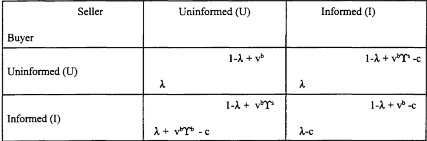
We first, consider the first stage payoffs. They are given by,

Table I: Payoffs in the First Stage (e<1I2)

SeIler Uninformed (U) Informed (1)

Buyer

l-À

+

v'T-c Uninformed (U)

l-À

+

v'T l-À+V'-c

Informed (I)

À+ vT-c À-c

The functions

Ti

j= b,s are defined in Appendix B. To make the information acquisition problem non-trivial we assume that the cost of information is less than the value of the gains from trading the indivisible good. Thus, we assume c<evb. If ｣ｾ･ｶ｢Ｌ＠ it foIlows that the uni que Nash

equilibrium is (U,U).

Our main characterization result is:

•

stage equilibrium strategies are (U,U). (As before we first denote the buyers' strategy.) If c<eV>, there exists values ofk denoted k)(c) and k₂(c) such that,

i) _{k)(c) < kj< k2(c), k)(c) is decreasing in c and converges to O as c goes to zero; k2}(c) is increasing in c and converges to 00 as c goes to zero.

ii) For k E [O,k)(c)), the uni que symmetric Nash equilibrium strategies are (U,U).

iii) For k = k)(c) there are two pure strategy Nash equilibria. The Nash equilibrium strategies are given by (U,O) and (I,U). In addition, there are infinitely many mixed strategy Nash equilibria. The equilibrium strategies are given by any lotteries over {I,U} on the part of the buyer, and the lottery that puts mass one on O on the part ofthe seller.

iv) For k E (k)(c),k₂(c)) there are no pure strategy Nash equilibria. There exists a unique

mixed strategy equilibrium, and the equilibrium strategies are characterized by the following probabilities that buyers (nb) and sellers (nS) are informed (i.e. they choose I),

nb(k) = [(c/vb_{)+(1-r(U,I,k))]I[(I-r(I,U,k)) +(I-r(U,I,k))].}

nS(k) = [v"Y"(I, O ,k )-c ]/vT(I, U ,k).

v) For ｫｾｫＲＨｃＩ＠ there is a unique Nash equilibrium. The equilibrium strategies are (U,O)

Proo! See Appendix C.

In the region in which monetary policy is not too volatile (k < k)(c)), even an informed seller who couId extract all the surplus would choose to be uninformed. The "Iost" surplus is not toe large. Similarly, in this region, the cost ofinformation exceeds the gains to a potential buyer even ifhe is assured to meet an uninformed seller (the only case in which he is able to extract part of the surplus). It follows that neither buyers nor sellers will choose to become informed. In this region information is "intrinsically" not very valuable; that is, its low value depends on being elose to certainty, and not on the players' strategies. At the point k=k)(c), buyers are indifferent between acquiring information and remaining uniformed. At this point, the gains from being informed (which accrue ifthey meet an uninformed seller) just offset the cost. Thus there are two pure strategy Nash equilibria and a continuum of mixed strategy equilibria.

For higher values ofk --more specificalIy for k)(c)<k<klc)-- there are no pure strategy equilibria. At the lower end ofthis region (low volatility) a large fraction ofthe buyers are informed (how large is depends on ｫｾ［＠ ｩｦｫｾ＾ｫＩＨ｣Ｉ＠ large is 100%), since the gains from being informed when meeting an uninformed seller exceed the cost. On the other hand, almost none of the sellers is informed. The reason is that, for k elose to k)(c), sellers do not stand to gain at alI from acquiring information: the potential gain is equal to the cost since they are going to meet informed buyers with probability one. In general, as k increases, the fraction ofbuyers who are informed decreases. The fraction of informed sellers increases up to the point k=kj, and then

decreases. To understand the increase in the region k)(c)<k<kj, note that in this region all pairs ofbuyers and sellers, except possibly (this depends on the value ｯｦｫｾＩ＠ for the case ofinformed sellers meeting uninformed buyers, trade the indivisible good with probability one. Increases in k in this sub-region redistribute income from uninformed sellers to informed buyers. Since sellers get all the "realized" surplus (i.e. buyers get zero in this region, but again depending on ｫｾ＠ trade will not occur with probability one and hence, there will be some lost surplus) whenever they are informed, the incentives that they have to limit the amount of redistribution lie at the heart of their decision to become informed. In this sub-region, the bigger the value of k the larger the • amount redistributed when they meet an informed buyer and, hence, the larger the number of

informed sellers. In the sub-region defined by kj< k <k₂(c), the gains from being informed are smaller because both when an informed buyer meets an uninformed seller, and an uninformed buyer meets an informed seller, trade wiIl not always occur. In fact, the probability oftrade for a pair (I,U) decreases with k, and so do the benefits from becoming informed.

For values ofk exceeding k₂(c), the private gains from becoming informed are too small, and the unique Nash equilibrium is (U,U). The reason for this is however quite different from the low k case. In this region there are two cases. First, the potential gain to a buyer from being informed for a given fixed strategy on the part of uninformed sellers is increasing in k. The problem is that uninformed sellers choose increasingly higher prices (we are in the increasing region ofthe price function in Figure 1) and, thus, reduce the probability oftrade. Thus, it is because ofthe

equilibrium response of sellers that buyers find it optimal not to pay for information. In some sense this is an example in which two wrongs produce a right. The first wrong corresponds to a policy that increases uncertainty. The second can be associated with the sellers desire to maintain their monopolist position and the consequent high prices that they charge. In the case of an informed seller meeting an uninformed buyer, it is clear that buyers have no incentive to acquire information (they get no surplus in that case) and, hence, sellers do not choose to become informed.

The distribution of information --in the case of intermediate leveIs of variability of the money supply-- is not degenerate. Moreover, the region in which some agents actively acquire information increases as the cost of acquiring information decreases.

5. Comparative Statics with Endogenous Information

The previous section established the existence of an equilibrium. It tums out that to characterize the equilibrium it is necessary to know that value ｯｦｫｾ＠ relative to the interval (k)(c),k₂(c». The case in which the probability oftrade is highest corresponds to a high ｫｾ＠ (see Proposition 3.2.1), and this is the case that we discuss in this section. Formally, our results assume that ｫｾ＾＠ k₂(c). For this case we fully explore the impact upon the equilibrium behavior of changes in the

variability ofthe monetary policy process as measured by k. We concentrate on the case in which

it is worthwhile to acquire information (c<evb_{). If this last inequality is violated the unique}

•

The Distribution of Information

How does policy uncertainty affect the equilibrium amount ofinformation? In the context ofthis modeI, an appropriate measure is given by the total fraction of the population that is informed. In addition to its impact on the overalI fraction of people informed, changes in k affect the identity ofthose informed. Given Theorem 4.1 it is cIear that no agents are informed ifkE [O,k\(c» U [k2(c), 00). Thus, we restrict attention to the set [k\(c),k2(c». The folIowing proposition

summarizes our results .

Proposition 5.1 Let e<1I2, and assume that c<evb. Then the distribution ofinformation satisfies

i) Aggregate information (nb(k)+nS(k»/2:

a) (nb(k)+nS(k»/2 E [0,1/2] for k=k\(c), b) (nb(k)+nS(k»/2 = Y2 for k\(c) ｾ＠ k ｾｫｴＬ＠

c) (nb(k)+nS(k) )/2 E (112,112 { 1-e( 1-q(l, U ,k2( c) )/[ (c/vb)+ 1-e( l-q(l, U ,kl c»]} ) for

kt<k<klc). Moreover, (nb(k)+nS(k»/2 is decreasing in this region.

ii) Individual information:

Proof

a) nb(k\(c»=l, 0<nb(k2(c»<1, and nb(k) is decreasing in k,

b) nS(k\(c» = nS(k₂(c» = O. The function nS(k) is increasing for k<kt and decreasing for k>kt·

It follows from the results in Theorem 4.1 once one notes that for ｫｾ＠ > k2(c), l=YS(U,I,k)] and an

informed selIer who meets an uninformed buyer gets alI the surplus since they exchange the good with probability one. In this region nb(k) = c/[vb(l-YS(l,U,k»]. Moreover, for k<kt, l=YS(l,U,k) +T'(I,U,k). The monotonicity results folIow from the properties ofthe Tj(l,U,k) functions derived in Appendix B.

•

The behavior of the different measures of information is illustrated in Figure 2. First, note that the total fraction of informed agents is a non-monotonic function of our measure of variability --the variance of--the money supply. At low leveIs ofk it is zero; itjumps to Y2 of--the population for moderate k's and it remains constant up to the point in which the equilibrium strategies for the pair (Informed buyer, Uninformed selIer) caIl for trading with probability less than one. At this point --which corresponds to kt-- the fraction of informed individuaIs decreases. It is zero for large k's.

..

k.(c» and the fraction ofinformed sellers is low (it is 0% at k.(c». In this region oflow k's--more precisely in the interval [k.(c),kj]-- the indivisible good is traded with probability one. The buyers have a huge incentive to acquire information because --whenever they are informed-- they can get better deals from the seller (who wants to charge a low price to guarantee a sale). No such a deal is given to uninformed buyers. As k increases, the value of the transfer increases. This makes sellers more willing to invest in information (informed sellers capture all the surplus), and buyers less willing to do so (they only obtain a surplus when they meet an uninformed seller, and the fraction of uninformed sellers is decreasing). This rei ative behavior continues over the range in which the good is traded with probability one, and the only issue is the allocation of the surplus between the two parties. For larger values ofk in the region in which information is acquired --formally in the interval [kj ,k₂₍ c) )-- the indivisible good is not traded alI the time whenever an informed buyer meets an uninformed seller. Thus, from the point of view of the buyer, the returns from being informed decrease and, consequently the fraction of informed buyers decreases. Since the threat of informed buyers is decreasing, and the gain from selling is decreasing as well, the sellers' best response is to reduce their demand for information. Thus, the fraction of both sellers and buyers that acquires information declines.

For high k's the equilibrium is such that no agent finds advantageous to acquire information. This is probably the consequence of our static model. In a dynamic setting one can think of the money supply at t as given by Mt =

Mo

+ í,J=oxj . In such a setting, the relevant variable is the last

piece of information. Note that the variance of the prior distribution of Mt increases with the length of the period in which the agents have chosen not to acquire information. Thus, it is possible that in such a model individuais would acquire information after a certain number of periods. In our static framework being uninformed means being equally uninformed. In a dynamic framework, the "age" of the last piece of information is relevant to determine the "degree" of information.

The Effects on Income and Welfare

What happens to welfare and income as k changes? In this setting it seems natural to describe welfare as given by the function W --as defined in sections 2 and 3-- minus the costs of acquiring information. If the costs of acquiring information are just waste of resources, this measure

corresponds to real income as well. In the region in which the equilibrium is in mixed strategies we use the probabilities assigned to each information option to construct the probability of a meeting with information set (ij). Since we assume a large number ofbuyers and sellers, these probabilities are also fractions ofthe population. We then have the following characterization of real income.

Proposition 5.2 Let e<1I2, and assume that c<evb. Let welfare (and real income) be defined by

I(k) = W(k) - c[1tb(k)+1tS_{(k)]. Then,}

i) I(k)=1 +vb, for k<k.(c),

•

iii) _{l(k)=I +vb-c for kl(c)<k<k2}(c), iv) l(k)=l+vb for k>k₂(c).

Proa! In case i), the uni que equilibrium is (U,U). Thus there are no costs ofacquiring

infonnation. Since the pai r (U,U) trades the indivisible good with probability one, real income is maximized. Case ii) corresponds to case ii) in the statement ofTheorem 4.1. Ifthe equilibrium is (U,U), there are no income losses. On the hand, if alI buyers choose to be infonned, real income is 1 +vb-c. Since any mixed strategy equilibrium in which the buyers randomize between these two strategies is an equilibrium as welI, any value of real income in [1 +vb, 1 +vb-c] can be an equilibrium outcome.

To prove iii) it is useful to separately prove the results for the subsets (kl(c),kt] and [kt,kic». First, consider the subset (kl(c),kj]. It is necessary to compute 1tb(k)+1tS_{(k). From the result in}

Proposition 5.1, it can be verified that 1tb(k)+1tS_{(k)=1. The claim then folIows from the}

observation that in the region ｫｾｫｪＬ＠ and for alI pairs of infonnation, the probability of trade q(k,e) equals one. Next, we consider the region [kt ,kzCc». Here the situation is more complicated. A fraction 1tb(1-1tS

) ofalI pairs have infonnation set (I,U). Income --ignoring

infonnation costs for now-- in this case is given by Proposition 3.3 and equals 1 +vb( I-e( I-q». In the other three cases --which, of course, occur with probability 1- 1tb(I-1tS

)--income is just 1 +vb.

Thus, average income is,

We wilI show that c(1-1tb-1tS_{)=vbe(I-q) 1tb(I-1t}S_{).To do this we calculate 1tb+1t}s _{for this subset.}

Using the results in Theorem 4.1 and Appendix B, it folIows that I-'r=T"e(1-q). Thus,

1tb=c/[vb(I-'fS)], and ＱＭＱｴｾ｣ＯＨｶｨｔＢＩＮ＠ Using these values it folIows that c(I-1tb-1tS_)=vbe(I-q)

1tb(1-1tS

) ifand only if(1!T")-(lI(1-'fS»=e(l-q)/[T"(1-'fS)]. This holds since I-'r=T"e(l-q).

Finally, note that in the region corresponding to iv) the unique Nash equilibrium is (U,U). Thus, the same reasoning as in i) establishes the desired result.

•

lO

ca1culate Y(k) given the previous result. It is given by,

Y(k)

l+vb ,

1 +vb-vbe(l-q(k))1tb(k)(1-1tS(k))

l+vb

for ｫｾｫｴ＠

for ｫｪｾｫ＼ｫＲＨｃＩ＠

for ｫＲＨｃＩｾｫＮ＠

Note that, using this definition, the variability ofthe money supply has no effect up to kt and then the appropriate measure of loss of output is the difference in the valuation of the indivisible good between buyers and sellers (vbe) multiplied by the probability ofnot trading (1-q(k)), and weighted by the frequency ofthis pairo

Figure 3 displays the behavior ofboth measures ofincome as a function ofk.

The Behavior of Prices

How do prices behave? For small values ofk, prices ofthe indivisible good are unresponsive to monetary shocks and identical in a cross sectional sample of pairs of buyers and sellers. Both buyers and sellers choose to be uninformed and prices are at the low end of the feasible intervalo As pointed out in section 3, prices decrease with increases in the variance ofthe money supply. In this region the ratio ofthe standard deviation ofprices and money supply Op(k)/OM(k) is zero: prices are unresponsive to money supply shocks.

For values ofk in the interval [k.(c),k2(c)), the equilibrium is in mixed strategies. In this region, each information pair trades at different prices. Thus, the model predicts that the cross-sectional variability ofprices is positive. This agrees with the findings by Eden (1994) and the studies collected by Sheshinski and Weiss (1993) in which more variable inflation is associated with more variability ofintra period prices. The distribution ofprices is given by,

(I,U) vbm* max{(e2m*k_l)/(2m*ke2m*k), (1-2ef' (e2m*k_l)/2m*k}, with probability 1tb(1-1ts).

(1,1) vbM with probability 1tb 1tS

•

Given k and the realization of M, the average price of the indivisible good over all the trading pairs (of course, we assume that there are a large number of buyers and sellers so that

probabilities equal fractions ofthe population) is ofthe form,

where (X.=V'1tb1tS