BAYESIAN AND CLASSICAL INFERENCE FOR THE GENERALIZED GAMMA DISTRIBUTION AND RELATED MODELS

UNIVERSIDADE FEDERAL DE SÃO CARLOS CENTRO DE CIÊNCIAS EXATAS E TECNOLOGIA

PROGRAMA INTERINSTITUCIONAL DE PÓS-GRADUAÇÃO EM ESTATÍSTICA UFSCar-USP

PEDRO LUIZ RAMOS

BAYESIAN AND CLASSICAL INFERENCE FOR THE

GENERALIZED GAMMA DISTRIBUTION AND RELATED

MODELS

Doctoral dissertation submitted to the Des/UFSCar and to the Institute of Mathematics and Computer Sciences – ICMC-USP, in partial fulfillment of the requirements for the PhD degree Statistics – Interagency Program Graduate in Statistics UFSCar-USP.

Advisor: Prof. Dr. Francisco Louzada

UNIVERSIDADE FEDERAL DE SÃO CARLOS CENTRO DE CIÊNCIAS EXATAS E TECNOLOGIA

PROGRAMA INTERINSTITUCIONAL DE PÓS-GRADUAÇÃO EM ESTATÍSTICA UFSCar-USP

PEDRO LUIZ RAMOS

ANÁLISE CLÁSSICA E BAYESIANA PARA A DISTRIBUIÇÃO

GAMA GENERALIZADA E MODELOS RELACIONADOS

Tese apresentada ao Departamento de Estatística – Des/UFSCar e ao Instituto de Ciências Matemáticas e de Computação – ICMC-USP, como parte dos requisitos para obtenção do título de Doutor em Estatística - Programa Interinstitucional de Pós-Graduação em Estatística UFSCar-USP.

Orientador: Prof. Dr. Francisco Louzada

To my beloved son, Francisco, and my wife and best friend, Maysa,

without whom this thesis would have been

ACKNOWLEDGEMENTS

There are a number of people without whom this thesis might not have been written, and to whom I am greatly indebted.

To my mother, Rita, who has been a source of encouragement and inspiration to me throughout my life. To my meemaw, Carmen, who always made me feel that she had been waiting to see me all day, and when she sees me, her day is completed.

To my beloved and supportive wife, Maysa, who is always by my side making my life worth living. To my little boy, Francisco, the most beautiful chapter of my life.

I would like to thank my brother, Eduardo, an excellent mathematician who supported me and helped in many topics of this thesis. To my father, Luiz, who always gave me the best things in life: his time, his care and his love. To my sisters Lais and Ana Luiza, more precious than gold.

I owe my deepest gratitude to my supervisor Dr. Francisco Louzada. Without his continuous optimism concerning this work, enthusiasm, encouragement and support this study would hardly have been completed.

I express my warmest gratitude to Wally and Eddie for opening their hearts and their house during my sandwich doctorate period. No matter where this life takes us, I hope that I will always hold a special place in all of their hearts because they certainly will in mine.

I would like to express my gratitude for the valuable suggestions from my committee members: Dr. Vera L. D. Tomazella, Dr. Helio S. Migon, Dr. Francisco A. Rodrigues and Dr. Teresa C. M. Dias.

I express my warmest gratitude to Dr. Dipak K. Dey who received me at UCONN and contributed to many discussions that helped to shape this thesis. I also would like to express my gratitude to Professor Dr. Victor H. Lachos for all that he has done. I consider him my friend.

Curiosity. Not good for cats,

great for scientists.

ABSTRACT

RAMOS, P. L.Bayesian and classical inference for the generalized gamma distribution and related models. 2018. 141 p. Tese (Doutorado em Estatística – Programa Interinstitucional

de Pós-Graduação em Estatística) – Instituto de Ciências Matemáticas e de Computação, Universi-dade de São Paulo, São Carlos – SP, 2018.

The generalized gamma (GG) distribution is an important model that has proven to be very flexible in practice for modeling data from several areas. This model has important sub-models, such as the Weibull, gamma, lognormal, Nakagami-m distributions, among others. In this work, our main objective is to develop different estimation procedures for the unknown parameters of the generalized gamma distribution and related models (Nakagami-m and gamma), considering both classical and Bayesian approaches. Under the Bayesian approach, we provide in a simple way necessary and sufficient conditions to check whether or not objective priors lead proper posterior distributions for the Nakagami, gamma, and GG distributions. As a result, one can easily check if the obtained posterior is proper or improper directly looking at the behavior of the improper prior. These theorems are applied to different objective priors such as Jeffreys’s rule, Jeffreys prior, maximal data information prior and reference priors. Simulation studies were conducted to investigate the performance of the Bayes estimators. Moreover, maximum a posteriori (MAP) estimators for the Nakagami and gamma distribution that have simple closed-form expressions are proposed Numerical results demonstrate that the MAP estimators outperform the existing estimation procedures and produce almost unbiased estimates for the fading parameter even for a small sample size. Finally, a new lifetime distribution that is expressed as a two-component mixture of the GG distribution is presented.

Keywords: Generalized gamma distribution, Nakagami-m distribution, gamma distribution,

RESUMO

RAMOS, P. L.Análise clássica e Bayesiana para a distribuição gama generalizada e mode-los relacionados. 2018. 141p. Tese (Doutorado em Estatística – Programa Interinstitucional

de Pós-Graduação em Estatística) – Instituto de Ciências Matemáticas e de Computação, Universi-dade de São Paulo, São Carlos – SP, 2018.

A distribuição gama Generalizada (GG) possui um papel fundamental para modelar dados em diversas áreas. Tal distribuição possui como casos particulares importantes distribuições, tais como, Weibull, Gama, lognormal, Nakagami-m, dentre outras. Nesta tese, tem-se como objetivo principal, considerando as abordagens clássica e Bayesiana, desenvolver diferentes procedimentos de estimação para os parâmetros da distribuição gama generalizada e de alguns dos seus casos particulares dentre eles as distribuições Nakagami-m e Gama. Do ponto de vista Bayesiano, iremos propor de forma simples, condições suficientes e necessárias para verificar se diferentes distribuições a priori não-informativas impróprias conduzem a distribuições posteriori próprias. Tais resultados são apresentados para as distribuições Nakagami-m, gama e gama generalizada. Assim, com a criação de novas prioris não-informativas, para tais modelos, futuros pesquisadores poderão utilizar nossos resultados para verificar se as distribuições a posteriori obtidas são impróprias ou não. Aplicações dos teoremas propostos são apresentados em diferentes prioris objetivas, tais como, a regra de Jeffreys, priori Jeffreys, priori maximal data information e prioris de referência. Iremos também realizar estudos de simulação para investigar a influência destas prioris nas estimativas a posteriori. Além disso, são propostos estimadores de máxima a posteriori em forma fechada para as distribuições Nakagami-m e Gama. Por meio de estudos de simulação verificamos que tais estimadores superam os procedimentos de estimação existentes e produzem estimativas quase não-viciadas para os parâmetros de interesse. Por fim, apresentamos uma nova distribuição obtida considerando um modelo de mistura de distribuições gama generalizada.

Palavras-chave: Distribuição Gama Generalizada, Distribuição Nakagami-m, Distribuição

LIST OF FIGURES

Figure 1 – Different shapes for the hazard function. . . 28 Figure 2 – TTT-plot shapes, retrieved from Ramos, Moala and Achcar (2014). . . 29 Figure 3 – Hazard function shapes for NK distribution considering different values of µ

andΩ. . . 40 Figure 4 – Mean residual life function shapes for NK distribution considering different

values ofµ andΩ. . . 41

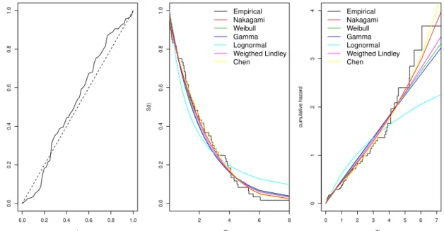
Figure 5 – TTT-plot, empirical reliability function and reliability function of different fitted probability distributions considering the data set related to the time of failure of 18 electronic devices and the cumulative hazard function. . . 54 Figure 6 – TTT-plot, empirical reliability function and reliability function of different

fitted probability distributions for the data set related to the number of 1000s cycles for failure for 60 electrical appliances and the cumulative hazard function. 56 Figure 7 – Survival function fitted by the empirical and by different probability

distribu-tions considering the data set related to the annual maximum discharges of the river Rhine at Lobith during 1901-1998 and the hazard function fitted by a GG distribution. . . 96 Figure 8 – MREs for µ considering c3= (2,2.1,···,4),µ =6,Ω=10,n=120 (left

panel)µ=20,Ω=2,n=20 (right panel) and forN=1,000,000 simulated samples andn=50. . . 105 Figure 9 – MREs, RMSEs forµ and Ωconsideringµ =4,Ω=2 forN =1,000,000

simulated samples andn= (10,15, . . . ,140). . . 105 Figure 10 – MREs, RMSEs forµ consideringµ =4,Ω=80 forN=1,000,000

simu-lated samples andn= (10,15, . . . ,140). . . 106 Figure 11 – MREs, RMSEs for different values of µ = (0.5,1.0, . . . ,20) considering

Ω=2 forN=1,000,000 simulated samples andn=50. . . 106 Figure 12 – MREs, RMSEs for different values of µ= (0.5,1.0,1.5, . . . ,20)considering

Ω=80 forN=1,000,000 simulated samples andn=50. . . 106 Figure 13 – MREs forφ consideringc3= (2,2.1,···,4),φ =3,λ =4 andn=20 (left

panel)φ =10,λ =4 and n=20 (right panel) forN=500,000 simulated

samples. . . 109 Figure 14 – MREs and RMSEs for different values ofφ = (0.5,1.0, . . . ,20)for sample

Figure 15 – MREs and RMSEs forφ for samples sizes of 6,7,8, . . . ,20 elements. Upper panels: consideringφ =4, lower panels: consideringφ =10. . . 110 Figure 16 – Density function shapes for GWL distribution considering different values of

φ,λ andα. . . 113 Figure 17 – Hazard function shapes for GWL distribution and considering different values

ofφ,λ andα . . . 115 Figure 18 – MRE’s, MSE’s related from the estimates ofφ =0.5,λ =0.7 andα =1.5

for N simulated samples, considering different values ofnobtained using the following estimation method 1-MLE, 2-MPS, 3-ADE, 4-RTADE. . . 121 Figure 19 – (left panel) the TTT-plot, (middle panel) the fitted survival superimposed to

the empirical survival function and (right panels) the hazard function adjusted by GWL distribution. . . 122 Figure 20 – (left panel) the TTT-plot, (middle panel) the fitted survival superimposed to

LIST OF TABLES

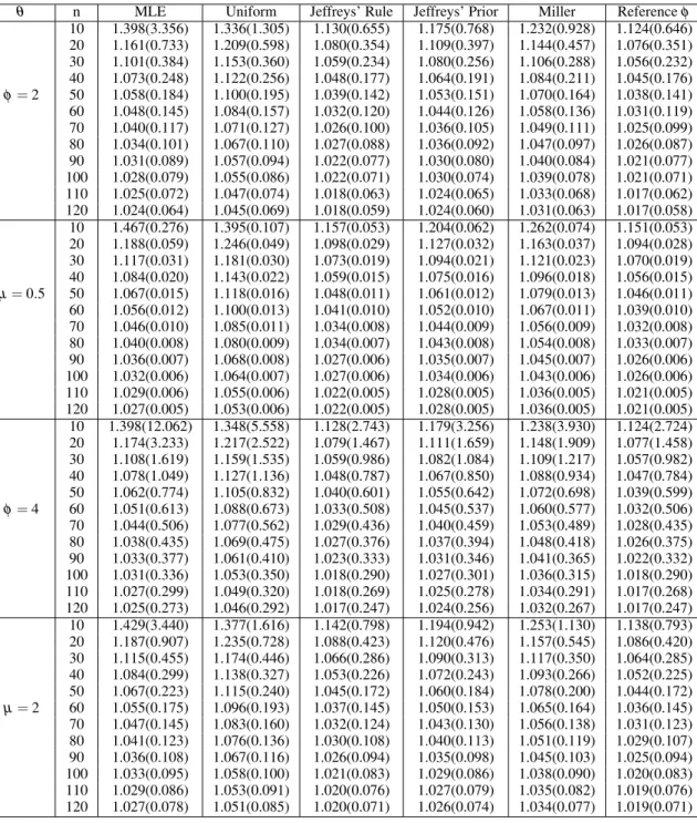
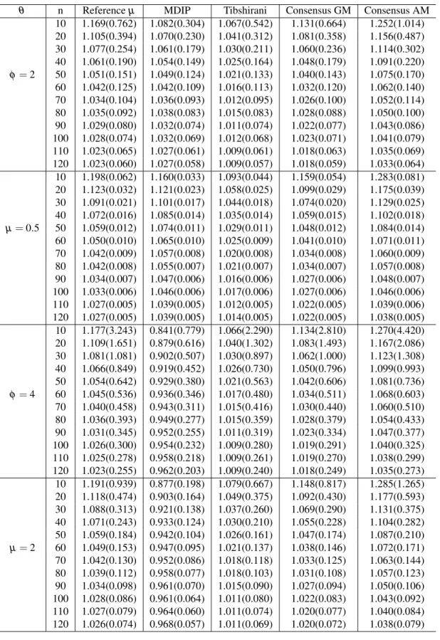
Table 1 – The MRE(MSE) from the estimates of µ considering different values of n withN=10,000,000 simulated samples using the estimation methods: 1

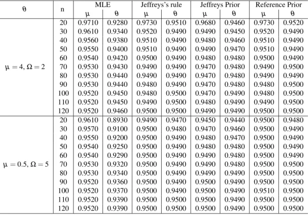
-MM, 2 - MLE, 3- Jeffreys’s rule, 4 - Jeffreys prior, 5 - Overall reference prior. 51 Table 2 – TheCP95% from the estimates ofµ andΩconsidering different values ofn

withN=10,000,000 simulated samples using the estimation methods: 1

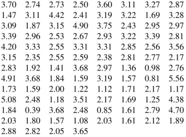
-MM, 2 - MLE, 3- Jeffreys’s rule, 4 - Jeffreys prior, 5 - Overall reference prior. 52 Table 3 – Data set related to the lifetime of one hundred observations on breaking stress

of carbon fibers . . . 53 Table 4 – The MLEs (Standard Errors) obtained for different distributions considering

the lifetime of one hundred observations on breaking stress of carbon fibers. . 53 Table 5 – Posterior mode and 95% credibility intervals forµ andΩobtained from the

data set related to the lifetime of one hundred observations on breaking stress of carbon fibers.. . . 53 Table 6 – Results of AIC, AICc and BIC criteria for different probability distributions

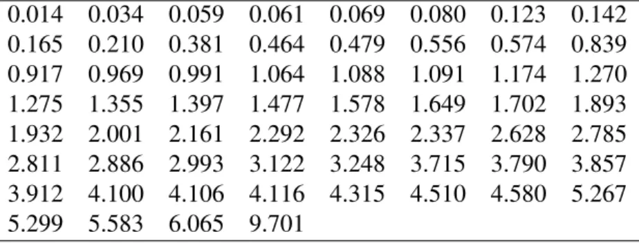
considering the data set related to the life time of one hundred observations on breaking stress of carbon fibers. . . 53 Table 7 – Data set related to the lifetime of 60 (in cycles) electrical devices. . . 54 Table 8 – The MLEs obtained for different distributions considering the lifetime data set

of 60 (in cycles) electrical devices. . . 55 Table 9 – Posterior mode and 95% CIs forµ andΩobtained from the data set related to

1000s cycles of failure for 60 electrical appliances. . . 55 Table 10 – Results of AIC, AICc and BIC criteria for different probability distributions

considering the data set related to 1000 cycles of failure for 60 electrical appliances. . . 55 Table 11 – The MRE(MSE) for for the estimates ofφ and µ considering different sample

sizes. . . 75 Table 12 – The MRE(MSE) for for the estimates ofφ and µ considering different sample

sizes. . . 76 Table 13 – TheCP95% from the estimates ofµ andΩconsidering different values ofn

withN=10,000 simulated samples. . . 77

Table 15 – Bias (RMSE) of the ML estimates and the Bayes estimators (posterior mode) for 10,000 samples of sizesn= (50,100,200)and different values ofθ. . . . 94 Table 16 – Coverage probability with a 95% confidence level equals the ML estimates

and the Bayes estimators (posterior mode) considering 10,000 samples of

sizesn= (50,100,200)and different values ofθ. . . 94 Table 17 – Posterior mean and 95% credibility intervals forφ and α from the data set

related to the annual maximum discharges of the river Rhine at Lobith during 1901-1998. . . 95 Table 18 – Posterior mode, standard deviations and 95% credible intervals forφ,µ andα

from the data set related to the annual maximum discharges of the river Rhine at Lobith during 1901-1998. . . 95 Table 19 – Results of AIC, AICc and BIC criteria for different probability distributions

considering the data set related to the annual maximum discharges of the river Rhine at Lobith during 1901-1998.. . . 95 Table 20 – Posterior mode, MLE, Posterior mean and 90% credibility intervals forφ and

α from the data set related to the annual maximum discharges of the river Rhine at Lobith during 1901-1998.. . . 96 Table 21 – Lifetimes data (in hours) related to a device put on test. . . 122 Table 22 – Results of AIC and AICc criteria and the p-value from the KS test for all fitted

distributions considering the Aarset dataset. . . 122 Table 23 – MLE estimates, Standard-error and 95% confidence intervals (CI) forφ,λ andα123 Table 24 – January average flows (m3_{/s) of the Cantareira system. . . . 123} Table 25 – Results of AIC and AICc criteria and the p-value from the KS test for all

CONTENTS

1 INTRODUCTION . . . 23

1.1 Objectives and Overview . . . 25

2 PRELIMINARIES . . . 27

2.1 Survival Analysis . . . 27

2.1.1 TTT-plot . . . 28

2.2 Frequentist inference . . . 29

2.2.1 Maximum Likelihood Estimation . . . 29

2.3 Bayesian Inference . . . 30

2.3.1 Non-informative priors . . . 30

2.4 Discrimination criterion methods . . . 33

2.5 Some Useful Mathematical Results . . . 33

3 NAKAGAMI-M DISTRIBUTION. . . 37

3.1 Introduction . . . 37

3.2 Nakagami-m distribution . . . 38

3.3 Classical Inference . . . 41

3.3.1 Moment Estimators . . . 41

3.3.2 Maximum Likelihood Estimation . . . 42

3.4 Bayesian Analysis . . . 43

3.4.1 Proper Posterior . . . 43

3.4.2 Jeffreys’s rule . . . 45

3.4.3 Jeffreys prior . . . 46

3.4.4 Reference prior . . . 47

3.4.5 Maximal Data Information prior . . . 48

3.4.6 Matching priors . . . 48

3.4.7 Numerical integration . . . 49

3.5 Simulation Study . . . 50

3.6 Applications in Reliability . . . 51

3.6.1 Breaking stress of carbon fibers. . . 52

3.6.2 Cycles up to the failure for electrical appliances . . . 54

3.7 Discussion. . . 56

4.1 Introduction . . . 59

4.2 Classical Inference . . . 60

4.3 Proper Posterior . . . 61

4.4 Objective priors . . . 65

4.4.1 Uniform Prior . . . 65

4.4.2 Jeffreys Rule . . . 66

4.4.3 Jeffreys prior . . . 66

4.4.4 Miller prior . . . 67

4.4.5 Reference prior . . . 68

4.4.5.1 Reference prior when φ is the parameter of interest . . . 68

4.4.5.2 Reference prior when µ is the parameter of interest . . . 69

4.4.5.3 Overall Reference prior . . . 69

4.4.6 Maximal Data Information prior . . . 70

4.4.6.1 Modified MDI prior . . . 70

4.4.7 Matching priors . . . 71

4.4.8 Consensus Prior . . . 72

4.4.8.1 Geometric mean . . . 72

4.4.8.2 Arithmetic mean . . . 73

4.5 Numerical evaluation . . . 74

4.6 Discussion. . . 78

5 GENERALIZED GAMMA DISTRIBUTION . . . 79

5.1 Introduction . . . 79

5.2 Maximum likelihood estimators . . . 80

5.3 Bayesian Analysis . . . 81

5.4 Objective Priors . . . 86

5.4.1 Some common objective priors . . . 86

5.4.2 Priors based on the Fisher information matrix . . . 87

5.4.3 Reference priors . . . 89

5.5 Simulation Analysis . . . 92

5.6 Real data application . . . 94

5.7 Discussion. . . 97

6 CLOSED-FORM ESTIMATORS FOR NAKAGAMI-M AND GAMMA DISTRIBUTIONS . . . 99

6.1 Introduction . . . 99

6.2 Closed-form estimators based on the generalized gamma distribution100 6.3 Nakagami-m . . . 101

6.3.1 Generalized moment estimators . . . 101

6.3.3 Maximum a Posteriori estimator . . . 102

6.3.4 Results . . . 104

6.4 Gamma distribution . . . 107

6.4.1 Bias corrected estimators . . . 107

6.4.2 Bias Expression . . . 108

6.4.3 Maximum a Posteriori estimator . . . 108

6.4.4 Simulation and Discussion . . . 108

6.5 Discussion. . . 110

7 MIXTURE OF GENERALIZED GAMMA DISTRIBUTION . . . 111

7.1 Introduction . . . 111

7.2 Generalized Weighted Lindley distribution . . . 112

7.2.1 Moments . . . 112

7.2.2 Survival Properties . . . 114

7.2.3 Entropy . . . 116

7.2.4 Lorenz curves. . . 118

7.3 Maximum likelihood estimators . . . 118

7.4 Simulation Study . . . 120

7.5 Application . . . 120

7.5.1 Lifetimes data . . . 121

7.5.2 Average flows data . . . 123

7.6 Concluding remarks . . . 124

8 COMMENTS AND FURTHER DEVELOPMENT . . . 125

8.1 Comments . . . 125

8.2 Further development . . . 126

BIBLIOGRAPHY . . . 129

23

CHAPTER

1

INTRODUCTION

In recent years, several new extensions of the exponential distribution have been proposed in the literature for describing real problems. Introduced byStacy(1962), the generalized gamma (GG) distribution is an important distribution that has proven to be very flexible in practice for modeling data from several areas, such as climatology, meteorology, medicine, reliability and image processing data, among others. The GG distribution is a distribution which has several particular cases, such as the exponential, Weibull, gamma, Log-normal, Nakagami-m, Half-normal, Rayleigh, Maxwell-Boltzmann and chi distributions.

Marani, Lavagnini and Buttazzoni(1986) used this distribution to analyze data relating to air quality in Venice, Italy.Tahai and Meyer(1999) proposed new methods for analyzing citations in recent publications to find journals with greater influence using the GG distribution.Aalo, Piboongungon and Iskander(2005) used this distribution to analyze the performance degradation of wireless communication systems.Liet al.(2011) used the GG distribution to obtain different

techniques for processing SAR (Synthetic aperture radar) images. Other applications of the GG distribution can be seen inNoortwijk(2001),Dadpay, Soofi and Soyer(2007),Balakrishnan and Peng(2006),Raju and Srinivasan(2002) andAhsanullah, Maswadah and Ali(2013).

The sub-models related to the GG distribution has been widely used in the literature. For instance, considering the Google scholarship, a search with the wordsWeibull distribution, gamma distribution,Log-normal distributionand Nakagami-m distribution, on March 2016,

found respectively 217.000, 2.920.000, 535.000 and 28.600 research papers.

24 Chapter 1. Introduction

BERNARDO,1992a;BERGER; BERNARDO,1992b;BERGER; BERNARDOet al.,1992; BERGERet al.,2015).

These objective priors are usually improper and could lead to improper posteriors. For instance, Noortwijk (2001) considered the non-informative Jeffreys prior to estimating the quartiles of the flood of a given river using the GG distribution. Such prior has the important one-to-one invariant property. However, we proved that such prior leads to an improper posterior and should not be used. Providing a proof that a posterior distribution is proper or improper is not an easy task.Northrop and Attalides(2016) argued that “. . .there is no general theory

providing simple conditions under which improper priors yields proper posteriors for a particular model, so this must be investigated case-by-case". In this study, we overcome this problem by providing in a simple way necessary and sufficient conditions to check whether or not these objective priors lead to proper posteriors distributions for the chosen models. In this way, one can easily check if the obtained posterior is proper or improper considering directly the behavior of the improper prior.

For the Nakagami distribution the main theorem is applied in different objective priors such as Jeffreys’s rule, Jeffreys prior, the MDI prior and reference priors. The Jeffreys-rule prior and Jeffreys prior gave proper posterior distribution respectively forn_≥1 andn_≥0, whereas

they are matching priors only for one of the parameters. The MDI prior provided improper posterior for any sample sizes and should not be used in Bayesian analysis. The overall reference prior yielded a proper posterior distribution if and only ifn_≥1. This prior is the one-at-a-time

reference prior for any chosen parameter of interest and any ordering of the nuisance parameters. It is also the only prior that is a matching prior for both parameters. An extensive simulation study showed that the proposed overall reference posterior distribution returns more accurate results, as well as better theoretical properties such as the invariance property under one-to-one transformations of the parameters, consistency under marginalization and consistent sampling properties. The proposed methodology is fully illustrated using two real lifetime data sets, demonstrating that the NK distribution can be used to describe lifetime data.

For the Gamma distribution we investigated the same problem related to the posterior distribution. We proved that among the priors considered in this study the MDI prior was the only that yield an improper posterior for any sample sizes. An extensive simulation study showed that the posterior distribution obtained under Tibshirani prior provided more accurate results in terms of mean relative errors (MREs), mean square errors (MSEs) and coverage probabilities and should be used to obtain inference for this distribution.

1.1. Objectives and Overview 25

was to consider reference priors. Since these priors are sensitive to the ordering of the unknown parameters, from Proposition2.3.1we obtained six reference priors, two of them were similar to other reference priors. Among the four distinct reference priors, we proved that only one returned a proper posterior distribution. The obtained posterior has excellent theoretical properties such as invariance property under one-to-one transformations of the parameters, consistency under marginalization and consistent sampling properties and should be used to make inference in the parameters of the GG distribution.

However, under the proposed approaches discussed so far, numerical integration must be used to obtain the posterior estimates and to perform the classical inference. Despite the enormous evolution of computational methods during the last decades, these methods still carry the disadvantage of high computational cost in many applications. Particularly in the case where the parameter estimators need to be obtained in real time, often within devices with embedded technologySong(2008). To overcome this problem we propose a class of maximum a posteriori (MAP) estimators for the parameters of the Nakagami and gamma distributions. They have simple closed-form expressions and can be rewritten as a bias-corrected maximum likelihood estimators (MLEs). Numerical results have shown that the MAP estimation scheme outperforms the existing estimation procedures and produces almost unbiased estimates for the parameters even for small sample size.

Finally, a new lifetime distribution that is expressed as a two-component mixture of the generalized gamma distribution is proposed. This generalization accommodates increasing, decreasing, decreasing-increasing-decreasing, bathtub, or unimodal hazard shapes, making such distribution a flexible model for reliability data. A significant account of mathematical properties of the new distribution is presented as well as two data sets are analyzed for illustrative purposes, proving that the mixture model outperforms several usual three parameters lifetime distributions.

1.1

Objectives and Overview

The main objective of this thesis is to improve the estimation procedures for the GG distribution and some of its related models. In order to achieved that we will:

1. Provide sufficient conditions to check whether or not objective priors lead to proper posteriors distributions for the Nakagami, gamma and GG distributions.

2. Derive different objective priors for the distributions cited above and apply the theorems to check if the obtained priors lead to proper posteriors.

26 Chapter 1. Introduction

4. Propose for the Nakagami and gamma distributions MAP estimators that have simple closed-form expressions for the parameters and can be rewritten as bias-corrected maxi-mum likelihood estimators.

5. Introduce and discuss the properties of a new lifetime distribution that is expressed as a two-component mixture of the generalized gamma distribution.

27

CHAPTER

2

PRELIMINARIES

In this section, we present a literature review of some important topics that are covered throughout this thesis.

2.1

Survival Analysis

In survival analysis, the responses are usually characterized by the failure times and the occurrence of censorship. These responses are usually measured over time until the occurrence of the event of interest. Therefore, a random variable (RV)T will have only non-negative values and

can be expressed by different mathematical functions, such as the probability density function (PDF) f(t), the cumulative distribution function (CDF) F(t), the survival function S(t), the hazard functionh(t), among others.

The probability density function of a non-negative RVT, is given by

f(t) = lim

∆t_→0

P(t_≤T _≤t+∆t)

∆t , f(t)≥0. (2.1)

The survival function with probability of an observation does not fail until the timet is

S(t) =P[T >t] =1₋P[T _≤t] =1₋

Z t

0 f(t)d(t) =1−F(t), 0<S(t)<1,

whereF(t)is cumulative distribution function.

The hazard function quantify the instantaneous risk of failure at a given time t and is given by

h(t) = lim

∆t_→0

P(t_≤T _≤+t∆t_|T _≥t)

∆t =

f(t)

28 Chapter 2. Preliminaries

Figure 1 – Different shapes for the hazard function.

Some useful relationships can be obtained from these functions, such as:

f(t) =h(t)S(t), h(t) = S ′_(t) S(t) =

∂

∂tlog(S(t)), S(t) =exp

−

Z t

0 h(t)dt

.

Glaser(1980) provided a helpful Lemma to study the behavior of the hazard function that is given as follow.

Lemma 2.1.1. Glaser(1980). Let T be a non-negative continuous random variable with twice

differentiable PDF, f(t_|θ). Then forη(t_|θ) =_−dtd logf(t_|θ), we have the following results:

1. Ifη(t_|θ)has a decreasing (increasing) shape, thenh(t_|θ)has an increasing (decreasing) shape.

2. Ifη(t_|θ)is bathtub (unimodal) shaped, thenh(t_|θ)is bathtub (unimodal) shaped.

2.1.1

TTT-plot

The TTT-plot (total time on test) is considered in order to verify the behavior of the empirical hazard function (BARLOW; CAMPO,1975). The TTT-plot is obtained from the plot of[r/n,G(r/n)]where

G(r/n) =

r

∑

ti+ (n−r)t(r)

!

/ n

∑

ti,

r=1, . . . ,n,i=1, . . . ,nandt_(r)is the order statistics. If the curve is concave (convex), the hazard

2.2. Frequentist inference 29

Figure 2 – TTT-plot shapes, retrieved fromRamos, Moala and Achcar(2014).

2.2

Frequentist inference

In a frequentist approach the unknown parameter vectorθ = (θ1, . . . ,θk)is considered

as having fixed but unknown values. Different classical inferential procedures are available in the literature, such as the maximum likelihood estimators, method of moments, L-moments, ordinary and weighted least-squares, percentile, maximum product of spacings, the maximum goodness-of-fit estimators, among others (LOUZADA; RAMOS; PERDONÁ,2016;BAKOUCH et al.,2017;DEYet al.,2017;RODRIGUES; LOUZADA; RAMOS,2018). In this work, the

maximum likelihood are considered to obtain the point and interval estimates under the classical approach.

2.2.1

Maximum Likelihood Estimation

The MLEs were chosen due to their good asymptotic properties. These estimators are obtained from maximizing the likelihood function (CASELLA; BERGER,2002). The likelihood function ofθ givent, is

L(θ,t) =

n

∏

f(ti|θ). (2.3)

For a model with k parameters, if the likelihood function is differentiable at θi, the

likelihood equations are obtained by solving the equations

∂ ∂ θi

log(L(θ,t)) =0,i=1,2, . . . ,k. (2.4)

Under mild conditions the solutions of (2.4) provide the maximum likelihood estimators. In many cases, numerical methods such as Newton-Raphson are required to find the solution of the nonlinear system. For large samples and under mild conditions they are consistent and efficient with an asymptotically multivariate normal distribution given by

ˆ

30 Chapter 2. Preliminaries

whereI(θ)is the Fisher information matrix,k_×kandIi j(θ)is the Fisher information element

ofθ iniand jgiven by

Ii j(θ) =E

− ∂

2

∂ θi∂ θj

log(L(θ,t))2

, i,j=1,2, . . . ,k. (2.6)

For large samples, approximated confidence intervals can be constructed for the indi-viduals parametersθi,i=1, . . . ,k, with confidence coefficient 100(1−γ)%, through marginal

distributions given by

ˆ

θi∼N[θi,I_ii−1(θ)]paran→∞. (2.7)

2.3

Bayesian Inference

So far, we have presented the estimation procedures using the frequentist approach. Bayesian analysis is an attractive framework in practical problems and became very popular in recent years. Here, we assume that the reader has a basic knowledge about Bayesian procedures. For an overview of Bayesian techniques, the reader is referred toMigon, Gamerman and Louzada (2014).

As the parameters are treated as random variables the distribution associated with such variables are known as prior distribution. The prior distribution is a key part of the Bayesian inference and there are different types of priors distribution available in the literature. Priors can be created using different procedures. For example, a prior distribution could be elicited from the assessment of an experienced expert (O’Haganet al.(2006)). On the other hand, we could

be interested in specifying a prior distribution, where the dominant information in the posterior distribution is provided by the data, such priors are known as noninformative prior. In this work, we considered different non-informative priors, such as the Jeffreys Rule (BOX; TIAO,1973), Jeffreys prior (JEFFREYS,1946), Maximal Data Information (MDI) prior (ZELLNER,1977; ZELLNER,1984) and Reference prior (BERNARDO,1979). These priors are usually improper and could lead to improper posteriors. Therefore, we investigated if whether these priors lead to proper posterior distributions for the chosen models.

2.3.1

Non-informative priors

2.3. Bayesian Inference 31

prior is given by

π(θ)∝

k

∏

1

θi

. (2.8)

In a further study,Jeffreys(1946) proposed his “general rule” in which the non-informative prior is obtained from the square root of the determinant of the Fisher information matrixI(θ) and θ is the vector of parameters. This prior has been widely used due to its invariance prop-erty under one-to-one transformations of parameters. For example, for any one-to-one function Φ=Φ(θ), the posterior p(Φ_|t)obtained from the reparametrized distribution f(t_|Φ)must be coherent with the posterior p(θ_|t)obtained from the original distribution f(t_|θ), in the sense that, p(Φ_|t) =p(θ_|t)_|dΦdθ_|.

The Jeffreys prior is obtained through the square root of the determinant of the Fisher information matrixI(θ)given by

π(θ)∝pdetI(θ). (2.9)

Zellner(1977) introduced another procedure to derive a noninformative priorπ(θ)in which the gain in the information supplied by the data is the largest as possible relative to the prior information, maximizing the information provided by the data. The resulting noninformative prior distribution is known as Maximal Data Information (MDI) prior and is defined as

π(θ)∝exp(Q(θ)), (2.10)

whereQ(θ)is the negative Shanon Entropy of f(t_|θ)given by

Q(θ) = Z

f(t_|θ)logf(t_|θ)dt, (2.11)

i.e, one measure of the information of f(t_|θ). The MDI prior has invariant limitations, in this case, is only invariant for linear transformations ofT orθ.

Another important noninformative prior was introduced byBernardo(1979) with further developments (BERGER; BERNARDO,1989; BERGER; BERNARDO, 1992a; BERGER; BERNARDO,1992b;BERGER; BERNARDOet al.,1992;BERGERet al.,2015). The proposed

reference prior is minimally informative in a precise information-theoretic sense. Moreover, the information provided by the data dominate the prior information, reflecting the vague nature of the prior knowledge. To achieve such prior the authors maximize the expected Kullback-Leibler divergence between the posterior distribution and the prior. The obtained reference prior provides a posterior distribution with interesting properties, such as:

∙ Consistent marginalization: For all datat, if the posterior p1(θ|t)obtained from

origi-nal model f(t_|θ,λ) is of the form p1(θ|t) = p1(θ|x)for some statistic x=x(t) whose

sampling distribution p(x_|θ,λ) = p(x_|θ)only depends onθ, then the posterior p2(θ|x)

32 Chapter 2. Preliminaries

∙ Consistent sampling properties: The properties under repeated sampling of the posterior distribution must be consistent with the model f(t_|θ)(COX; HINKLEY,1979).

∙ Invariant under one-to-one transformations: The same properties presented in the Jeffreys

prior section.

Bernardo(2005) presented different procedures to derive reference priors in the presence of nuisance parameters. The following propositions are useful to obtain the reference priors for the chosen models.

Proposition 2.3.1. Let f(x_|θ,λ)be a parametric model, whereθ is the parameter of interest,

λ = (λ1, . . . ,λm) is a vector of nuisance parameters and I(θ,λ)Fisher’s information matrix

(m+1)_×(m+1). It is assumed that the joint distribution of(θ,λ)is asymptotically normal with mean and covariance matrixS(θˆ,λˆ) =I−1(θˆ,λˆ), where(θˆ,λˆ)correspondents of MLEs. Moreover,Sjis a j×jupper left submatrix ofSandιi,j(θ,λ)is an element ofIj. If the nuisance

parameter spaces _∧i(θ,λ1, . . . ,λj−1) =∧i are independent of θ and λi’s and the functions

ι_i,i, . . . ,ι_m,m, i=1, . . . ,mfactorize in the form

s− 1 2

1,1(θ,λ) = f0(θ)g0(λ) and ι 1 2

i+1,i+1(θ,λ) = fi(λi)gi(θ,λ−i).

whereλ₋i= (λ1, . . . ,λi₋1,λi+1, . . . ,λm). Then

π(θ)∝ f0(θ), π(λi|θ,λ−i)∝ fi(λi),i=1, . . . ,m, (2.12)

and the reference prior when θ is the parameter of interest and λ is the vector of nuisance parameters is given byπθ(θ,λ) = f0(θ)∏mi=1 fj(λi).

Proposition 2.3.2. (BERGERet al.,2015, p.196) Consider the unknown vector of parameters

θ = (θ1, . . . ,θm)and the posterior distribution p(θ|t)with asymptotically normal distribution

and dispersion matrixS(θ) =I−1(θ). IfI(θ)is of the form

I(θ) =diag(f1(θ1)g1(θ−1), . . . ,fm(θm)gm(θ−m)),

where fi(·)andgi(·)are positive functions ofθifori=1, . . . ,m, then the one-at-a-time reference

prior, for any chosen parameter of interest and any ordering of the nuisance parameters in the derivation, hereafter, the overall reference prior is given by

π(θ) =pf1(θ1). . .fm(θm). (2.13)

Tibshirani(1989) proposes an alternative method to derive a class of non-informative priorsπ(θ₁,θ₂)whereθ₁is the parameter of interest so that the credible interval forθ₁has a coverage errorO(n−1) in the frequentist sense, i.e.,

2.4. Discrimination criterion methods 33

whereθ₁1−α(π;X)_|(θ1,θ2)denote the(1−α)th quantile of the posterior distribution ofθ1. The

class of priors satisfying (2.14) are known as matching priors.

To achieve this, Tibshirani (1989) proposed to reparametrize the model in terms of the orthogonal parameters (δ,λ) in the sense discussed by Cox and Reid (1987). That is,

I_δ,λ(δ,λ) =0 for all (δ,λ), where δ is the parameter of interest and λ is the orthogonal nuisance parameter. Thus, the matching priors are all priors of the form

π(δ,λ) =g(λ)pI_{δ δ}(δ,λ), (2.15)

whereg(λ)>0 is an arbitrary function andI_{δ δ}(δ,λ) is theδ entry of the Fisher information matrix. Further,Mukerjee and Dey(1993) discussed sufficiency and necessary conditions for a class of Tibshirani priors be matching prior up too(n−1).

2.4

Discrimination criterion methods

In situations that involve uncertainty measures, discrimination criterion methods are of great importance in statistical analysis as a goodness of fit for model selection. Let k be

the number of parameters to be fitted and ˆθ is the estimate ofθ some discrimination criterion methods based on log-likelihood function are given by

∙ Akaike information criterion:AIC=₋2 log(L(θˆ;t)) +2k.

∙ Corrected Akaike information criterion:AICC=AIC+2_(nk(k+_−k−1₁)₎ .

∙ Bayesian information criterion:BIC=₋2 log(L(θˆ;t)) +klog(n).

Given observed data and a set of candidate models the best model is the one which provides the minimum values. These procedures includes penalty discourages overfitting, i.e, in-creasing the number of parameters with poor predictive results. For an overview of discrimination criterion methods, the reader is referred toBurnham and Anderson(2004).

2.5

Some Useful Mathematical Results

In this section, we present some useful propositions that are used to prove some posterior properties.

LetR+ denote the strictly positive real numbers.

Definition 2.5.1. Let g :U _→R+ and h :U _→R+, whereU _⊂R, and let_a∈R. We can say that g(x) ∝

x→ah(x)if

lim inf

x→a

g(x)

h(x) >0 and lim supx→a

g(x) h(x) <∞. We define the meaning of the relations g(x) ∝

x_→a+h(x)and g(x)_x→∝_a−h(x)fora∈

34 Chapter 2. Preliminaries

The following propositions and definitions are useful to prove the results related to the posterior distribution.

We denoted by R₌R_{∪ {−}∞,∞_} the extended real number linewith its usual order

(_≤), whileR+ denotes the strictly positive real numbers,R+₌R+_{∪ {}∞_}andR+₀ denotes the non-negative real numbers.

Definition 2.5.2. Let g :U _→R+and h :U _→R+, whereU _⊂R. We will say that g_(x)∝h(x) if there isc_0∈R+ and_c1∈R+ such that_c0h_(x)≤g_(x)≤c1h_(x)for every_x∈U.

Note that if for somec_∈R+we have lim_x→ag(x)

h(x) =c, then g(x)_x→∝_ah(x). The following

proposition relates Definition2.5.2and Definition2.5.1forU _{= (a,b)}.

Proposition 2.5.3. Let g :(a,b)_→R+and h :_(a,b)→R+be continuous functions on_(a,b)⊂R, wherea_∈Rand_b∈R. Then g_(x)∝h(x)if and only if g(x) ∝

x→ah(x)and g(x)x→∝bh(x).

Proof. Suppose g(x) ∝

x→ah(x)and g(x)x→∝bh(x). Then, by Definition2.5.1, lim infx→a

g(x) h(x)=w1 and lim sup_x→ag(x)

h(x) =w2 for somew1 and w2 both in (0,∞). Therefore, from the definition of liminf and limsup there is somea′_∈(a,b)such that w1

2 ≤

g(x) h(x)≤

3w2

2 for everyx∈(a,a′]. Analogously, there is somev1andv2, both in(0,∞),andb′∈(0,∞)such that v₂1 ≤ g_h(x)

(x) ≤ 3v2

2 for every v_∈[b′,b). On the other hand, since g(x)

h(x) is continuous in [a

′_,b′_{], the Weierstrass}

extreme value Theorem (RUDINet al.,1964) states that there is somex0andx1∈[a′,b′]such that

g(x1)

h(x1)≤

g(x) h(x)≤

g(x2)

h(x2)for everyx∈[a

′_,b′_{]. Finally, choosingm=min}

w1

2 ,

v1

2, g(x1)

h(x1)

>0 and

M=max

₃

w2

2 , 3v2

2 , g(x2)

h(x2)

<∞, it follows from the above considerations thatm_≤g(x)

h(x) ≤M for everyx_∈(a,b), which by Definition2.5.2means thatg(x)∝h(x).

Supposeg(x)∝h(x). By Definition 2.5.2, there are some m>0 andM<0 such that

m_≤g(x)

h(x) ≤Mfor everyx∈(a,b). This implies that

lim inf

x→a

g(x)

h(x) ≥m>0 and lim supx→a

g(x)

h(x) ≤M<∞,

which by Definition2.5.1means that g(x) ∝

x→ah(x). The proof that g(x)x∝→bh(x)is analogous to

the previous case.

2.5. Some Useful Mathematical Results 35

Proposition 2.5.4. Let g :(a,b)_→R+and h :_(a,b)→R+be continuous functions in_(a,b)⊂R, wherea_∈Rand_b∈R, and let_c∈(a,b). Then if g_(x) ∝

x→ah(x)or g(x)x∝_→bh(x)we have

Z c

a

g(t)dt ∝ Z c

a

h(t)dt or Z b

c

g(t)dt∝ Z b

c

h(t)dt.

Proof. Suppose g(x) ∝

x→ah(x). By continuity and non-nullity of g(x) and h(x) in c we have

g(x) ∝

x→ch(x). Therefore, by Proposition2.5.3, we have thatg(x)∝h(x)in(a,c). This implies

that

Z c

a

g(t)dt ∝ Z c

a

h(t)dt.

The proof of the case g(x) ∝

x→bh(x)is analogous.

The following propositions are useful to prove the results related to the posterior distribu-tion. LetR+ denote the positive real numbers andR+₀ denote the positive real numbers including 0.

Definition 2.5.5. Let g :U _→R+₀ and h :U _→R+₀, whereU _⊂R. We say that g_(x).h_(x) if there existM_∈R+ such that g_(x)≤Mh_(x)for every_x∈U. If g_(x).h_(x)and h_(x).g_(x) then we say that g(x)∝h(x).

Definition 2.5.6. Leta_∈R, g :U _→R+and h :U _→R+, whereU _⊂R. We say that g_{(x) .}

x→a

h(x)if lim sup_x→ag(x)

h(x)<∞. If g(x)x→.a

h(x)and h(x) .

x→a

g(x)then we say that g(x) ∝

x→ah(x).

The meaning of the relations g(x) .

x→a+

h(x)and g(x) .

x→a−

h(x)for a_∈Rare defined analogously.

Note that, if for somec_∈R+we have lim_x→ag(x)

h(x)=c, then g(x)x→∝ah(x). The following

proposition is a direct consequence of the above definition.

Proposition 2.5.7. For a_∈R and _{r ∈}R+ , let _{f1(x) .}

x→a

f₂(x) and g₁(x) .

x→a

g₂(x) then the following hold

f1(x)g1(x) .

x→a

f2(x)g2(x) and f1(x)r .

x→a

f2(x)r.

The following proposition relates Definition2.5.5and Definition2.5.6.

Proposition 2.5.8. Let g :(a,b)_→R+and h :_(a,b)→R+be continuous functions on_(a,b)⊂R, wherea_∈Rand_b∈R. Then g_(x).h_(x)if and only if g_{(x) .}

x→a

h(x)and g(x) .

x→b

h(x).

Proof. Suppose that g(x) .

x→a

h(x)and g(x) .

x→b

h(x). Then, by Definition2.5.6,

lim sup_x→ag(x)

h(x) =w for some w∈R

36 Chapter 2. Preliminaries

somea′_∈(a,b)such that g(x) h(x) ≤

3w

2 for everyx∈(a,a′]. Proceeding analogously, there must exist somev_∈R+ and_b′_∈(a′_,b)such that g(x)

h(x) ≤ 3v

2 for everyx∈[b′,b). On the other hand, since g(x)

h(x) is continuous in[a

′_,b′_{], the Weierstrass Extreme Value Theorem states that there}

exist some x1 ∈[a′,b′] such that g_h(x) (x) ≤

g(x1)

h(x1) for everyx ∈[a

′_,b′_{]. Finally, choosing M =}

max

₃

w

2 , 3v

2 , g(x1)

h(x1)

<∞, it follows that g(x)

h(x) ≤M for everyx∈(a,b), which by Definition 2.5.5means thatg(x).h(x).

Now supposeg(x).h(x). By Definition2.5.5, there exist someM<0 such that g(x)

h(x) ≤ M for everyx_∈(a,b). This implies that lim sup_x→ag_h(x)_{(x) ≤}M<∞which by Definition 2.5.6 means that g(x) .

x→a

h(x). The proof that g(x) .

x_→b

h(x)must also be satisfied is analogous to the previous case. Therefore the theorem is proved.

Note that if g :(a,b)_→R+ and h :_(a,b)→R+are continuous functions on_(a,b)⊂R, then by continuity it follows directly that limx→c

g(x) h(x) =

g(c)

h(c) >0 and therefore g(x)x→∝ch(x)

for everyc_∈(a,b). This fact and the Proposition2.5.8imply directly the following.

Proposition 2.5.9. Let g :(a,b)_→R+and h :_(a,b)→R+be continuous functions in_(a,b)⊂R, wherea_∈Rand_b∈R, and let_c∈(a,b). Then if g_{(x) .}

x→a

h(x)(or g(x) .

x→b

h(x)) we have that

Rc

ag(t)dt.

Rc

ah(t)dt (respectively

Rb

c g(t)dt.

Rb

37

CHAPTER

3

NAKAGAMI-M DISTRIBUTION

3.1

Introduction

The Nakagami-m (NK) distribution is a powerful statistical tool for modeling fading radio signals. Proposed byNakagami(1960), this model has received considerable attention due to its flexibility to describe a wide range of communication engineering problems. For instance, considering the IEEE Xplore digital Library, a search carried out using the word ”Nakagami” on April 2017 found 3,660 research papers.

The NK distribution has been used successfully in other fields such as medical imaging processing (SHANKARet al.,2001;TSUI; HUANG; WANG,2006), hydrologic engineering

(SARKAR; GOEL; MATHUR, 2009; SARKAR; GOEL; MATHUR, 2010), seismological analysis (CARCOLE; SATO,2009;NAKAHARA; CARCOLÉ,2010) and traffic modeling of multimedia data (KIM; LATCHMAN,2009). However, there are no comprehensive references in the literature which consider the NK distribution as a reliability model. In this chapter, we present the reliability properties for this model and also prove that its hazard rate (mean residual life) function presents increasing (decreasing) or bathtub (unimodal) shapes.

38 Chapter 3. Nakagami-m distribution

Cheng(2012) proposed a closed-form estimator for the fading parameter obtained as a limiting procedure of the traditional GM estimators. However, these estimators depend on the asymptotic properties to construct the confidence intervals.

Considering a Bayesian approach,Son and Oh(2007) discussed Bayes estimation using independent gamma prior distributions for the parameters of the NK distribution. However, Bernardo(2005) argued that using simple proper priors, presumed to be non-informative, often hides important unwarranted assumptions which may easily dominate, or even invalidate, the statistical analysis and should be strongly discouraged.Beaulieu and Chen(2007) discussed MAP estimators using informative priors. However, in applications, it is difficult to obtain prior information for the unknown parameters. To overcome this problem, a Bayesian analysis can be performed with non-informative priors, i.e., priors constructed by formal rules.

In this chapter, different objective priors for the NK distribution are presented such as Jeffreys’s rule, Jeffreys prior, the MDI prior and the reference prior. These priors are improper and could lead to improper posteriors. We propose a theorem that provides sufficient and necessary conditions for a general class of posterior to be proper posterior distributions. The proposed theorem is used to investigate if these priors lead to proper or improper posterior distributions. Later, a posterior distribution based on the reference prior is obtained. This proper posterior returns better numerical results and also excellent theoretical properties such as invariance property under one-to-one transformations of the parameters, consistency under marginalization and consistent sampling properties. The proposed posterior distribution also satisfies the matching prior properties for bothΩandµ. Finally, our methodology is illustrated using two real lifetime

data sets, proving that the NK distribution can be used to describe lifetime data.

The remainder of this chapter is organized as follows. Section 2 presents mathematical properties for the NK and reviews two common classical approaches. Section 3 presents the main theorem that provides sufficient and necessary conditions for a general class of posterior to be proper with applications in non-informative priors. In Section 4, a simulation study is presented in order to identify the most efficient estimation procedure. Section 5 presents an analysis of two lifetime data sets. Finally, Section 6 summarizes the study.

3.2

Nakagami-m distribution

LetT be a random variable with NK distribution, the PDF is given by

f(t_|θ) = 2 Γ(µ)

µ

Ω

µ

t2µ−1exp

−_Ωµt2

, (3.1)

for allt>0, whereθ = (µ,Ω),µ _≥0.5 andΩ>0 are, respectively, the shape (also known as a fading parameter) and scale parameters andΓ(φ) =R∞

0 e−xxφ−1dxis the gamma function. We

3.2. Nakagami-m distribution 39

Important probability distributions can be obtained from the NK distribution such as the Rayleigh distribution (µ =1) and the half-normal distribution (µ =0.5). Moreover, this model

is also related to the gamma distribution. For instance, ifY _∼Gamma(a,b), thenT =√Y has a

NK distribution with µ=aandΩ=ab. Due to this relationship, theµ parameter can also take

on values between 0<µ <0.5.

Let T be a continuous lifetime (non-negative) random variable with NK distribution. The raw moments are given as

E(Tr) = Γ(µ+r/2) Γ(µ)

Ω

µ

r/2

, (3.2)

forr_∈N. After some algebraic manipulation, the mean and variance of (3.1) are respectively given by

E(T) = Γ(µ+1/2) Γ(µ)

Ω

µ

1₂

and (3.3)

Var(T) =Ω 1₋

Γ(µ+1/2) Γ(µ)

2!

. (3.4)

The median and the mode of the NK distribution are

Med(T) =√Ω and Mode(T_|θ) =

√

2 2

(2µ₋1)Ω

µ

1₂

.

The reliability function that represents the probability that an observation does not fail untilt is

S(t_|θ) = 1 Γ(µ)Γ

µ,µ

Ωt 2

,

whereΓ(y,x) =R∞

x wy−1e−wdwis the upper incomplete gamma function. For the NK distribution,

the hazard function is given by

h(t_|θ) =2µ Ω

µ

t2µ−1exp

−_Ωµt2

Γµ,µ

Ωt 2−1

. (3.5)

Theorem 3.2.1. The hazard rate functionh(t_|θ)of the NK distribution is bathtub (increasing) shaped for 0<µ <0.5(µ _≥0.5), for allΩ>0.

Proof. Firstly

η(t_|θ) =₋d

dtlogf(t|θ) =−

(2µ₋1)

t −

2µt

Ω . (3.6)

40 Chapter 3. Nakagami-m distribution

The behavior of the hazard function (3.5) whent_→0 andt_→∞is given by

h(0_|θ) =

     

    

∞, ifµ<0.5

r

2

Ω, ifµ=0.5 0, ifµ>0.5

and h(∞_|θ) =∞.

Figure3presents examples for the shapes of the hazard function for different values of

µ andΩ.

0 2 4 6 8

0

1

2

3

4

5

t

h(t)

µ=0.05, Ω=0.5 µ=0.10, Ω=0.5 µ=0.20, Ω=1.0 µ=0.30, Ω=2.0 µ=0.40, Ω=4.0

0 2 4 6 8

0

1

2

3

4

5

t

h(t)

µ=0.7, Ω=5 µ=1.0, Ω=5 µ=2.0, Ω=10 µ=4.0, Ω=10 µ=5.0, Ω=10

Figure 3 – Hazard function shapes for NK distribution considering different values ofµandΩ.

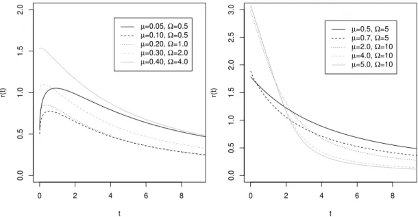
The mean residual life (MRL) represents the expected additional lifetime given that a component has survived until time t.

Proposition 3.2.2. The mean residual life functionr(t_|θ)of the NK distribution is given by

r(t_|θ) = 1 S(t_|θ)

Z ∞

t

y f(y_|θ))dy₋t =

s

Ω

µ

Γ µ+1₂,_Ωµt2 Γ µ,_Ωµt2

!

−t. (3.7)

The behaviors of the MRL function (3.5) whent_→0 andt_→∞are, respectively

r(0_|θ) =

s

Ω

µ

Γ µ+1₂

Γ(µ)

!

and r(∞_|θ) = 1

h(∞_|θ) =0.

The following Lemma is useful to obtain the shapes of the MRL function.

3.3. Classical Inference 41

1. Ifh(t_|θ)has a decreasing (increasing) shape, thenr(t_|θ)has an increasing (decreasing) shape (BRYSON; SIDDIQUI,1969) .

2. Ifh(t_|θ)is bathtub shaped and h(0)r(0)>1, thenr(t_|θ)is unimodal shaped (OLCAY, 1995).

Theorem 3.2.4. The mean residual life functionr(t_|θ)of the NK distribution has a unimodal (decreasing) shape for 0<µ <0.5(µ _≥0.5), for allΩ_>0.

Proof. For µ _≥0.5 andΩ>0,h(t_|θ)has an increasing shape. Then, by Lemma3.2.3,r(t_|θ) has a decreasing shape. ForΩ>0 and 0<µ<0.5,h(t_|θ)has a bathtub shape andh(0)r(0)>1.

Therefore, based on Lemma3.2.3,r(t_|θ)has a unimodal shape.

Figure4presents examples of the shapes of the mean residual life function for different values ofµ andΩ.

0 2 4 6 8

0.0

0.5

1.0

1.5

2.0

t

r(t)

µ=0.05, Ω=0.5 µ=0.10, Ω=0.5 µ=0.20, Ω=1.0 µ=0.30, Ω=2.0 µ=0.40, Ω=4.0

0 2 4 6 8

0.0

0.5

1.0

1.5

2.0

2.5

3.0

t

r(t)

µ=0.5, Ω=5 µ=0.7, Ω=5 µ=2.0, Ω=10 µ=4.0, Ω=10 µ=5.0, Ω=10

Figure 4 – Mean residual life function shapes for NK distribution considering different values ofµ andΩ.

3.3

Classical Inference

3.3.1

Moment Estimators

The method of moments (MM) is one of the oldest methods used for estimating pa-rameters in statistical models. Nakagami (1960) proposed the following moment estimators

ˆ

µ = ∑

n i=1ti2

2

n∑n_i=1t_i4₋ ∑n_i=1t_i22

and ˆΩ=1 n

n

∑

42 Chapter 3. Nakagami-m distribution

Note that the second moment of the NK distribution isΩ. Therefore, ˆΩ=∑n_i=1t_i2/nis

an unbiased estimator forΩ.

3.3.2

Maximum Likelihood Estimation

Let T₁, . . . ,Tn be a random sample such thatT ∼NK(Ω,µ). The likelihood function

from (3.1) is given by

L(θ_|t) = 2

n

Γ(µ)n

µ Ω nµ ( n

∏

t_i2µ−1

)

exp ₋µ Ω

n

∑

t_i2

!

. (3.9)

The log-likelihood function is

logL(θ_|t) =nlog(2)₋nlog(Γ(µ)) +nµlogµ Ω

+ (2µ₋1)

n

∑

log(ti)−

µ

Ω

n

∑

t_i2. (3.10)

The estimates are obtained by maximizing the likelihood function. From the expressions

∂

∂ΩlogL(θ|t) =0, ∂

∂ µ logL(θ|t) =0, the likelihood equations are given as

n1+logµ

Ω

−nψ(µ) +2

_∑

log(ti) = 1

Ω

n

∑

i=1

t_i2 (3.11)

and

−n_Ωµ + µ

Ω2

n

∑

t_i2=0, (3.12)

whereψ(k) = _∂k∂ logΓ(k) = Γ_Γ(k)′(k) is the digamma function. The MLE for ˆΩis

ˆ Ω=1

n

n

∑

t_i2. (3.13)

Substituting ˆΩin (3.11), the estimate for ˆµ can be obtained solving

log(µ)₋ψ(µ) =log 1 n

n

∑

t_i2

!

−2_n n

∑

log(ti). (3.14)

Under mild conditions, the MLE are asymptotically normally distributed with a joint bivariate normal distribution given by

(µˆMLE,ΩˆMLE)∼N2[(µ,Ω),I−1(µ,Ω))]forn→∞,

whereI(µ,Ω)is the Fisher information matrix

I(µ,Ω) =n



 

(µψ′(µ)₋1)

µ 0

0 µ

Ω2





, (3.15)

3.4. Bayesian Analysis 43

3.4

Bayesian Analysis

In this section, sufficient and necessary conditions are presented for a general class of posterior to obtain proper posterior distributions. Our proposed methodology is illustrated in different non-informative priors for parameters µ andΩof the NK distribution.

3.4.1

Proper Posterior

The joint posterior distribution forθ is equal to the product of the likelihood function

(3.9) and the joint prior distributionπ(θ)divided by a normalizing constantd(t), resulting in

p(θ_|t) = 1 d(t)

π(θ) Γ(µ)n

µ Ω nµ ( n

∏

t_i2µ−1

)

exp ₋µ Ω

n

∑

t_i2

!

, (3.16)

where

d(t) = Z

A

π(θ) Γ(µ)n

µ Ω nµ ( n

∏

t_i2µ−1

)

exp ₋µ Ω

n

∑

t_i2

!

dθ, (3.17)

and A _={(0_,∞)_×(0,∞)_}is the parameter space ofθ. For any prior distribution in the form

π(θ)∝π(µ)π(Ω), our purpose is to find sufficient and necessary conditions for the posterior to be proper, i.e.,d(t)<∞.

Theorem 3.4.1. Suppose the behavior ofπ(Ω)is given byπ(Ω)∝ Ωk, fork_∈Rwith_k>−1 and π(µ)is strictly positive. Then, the posterior distribution (3.16) is improper. On the other hand, suppose that the behavior ofπ(Ω)andπ(µ)is given by

π(Ω)∝ Ωk, π(µ) ∝

µ→0+ µ

r0 _{and π(µ) ∝}

µ→∞µ r∞_,

for k_∈Rwith_{k≤ −}1,_r0∈Rand_r∞∈R. Then, the posterior distribution (3.17) is proper if and only ifn>₋r0in casek=−1, and is proper if and only ifn>−r0−k−2 in casek<−1.

Proof. LetB_={(0_,∞)×(0_,∞)}and consider the change of coordinates through the transfor-mationθ :B_→A

θ(φ,λ) = (µ(φ,λ),Ω(φ,λ)) =

φ,φ

λ

. (3.18)

Note thatA _=θ(B₎. Since_|det_{(Dθ(φ,λ))|=φ λ}−2(where_Dθ(φ,λ)is the Jacobian matrix of the functionθ(φ,λ)), denotingΘ= (φ,λ)and applying the Theorem of Change of Variables on the Lebesgue integral (FOLLAND,1999), we have that

d(t)∝ Z

A

Ωk_π(µ)

Γ(µ)n

µ Ω nµ ( n

∏

t_i2µ

)

exp ₋µ Ω

n

∑

t_i2

!

dθ

= Z

B

φk+1π(φ)λnφ−k−2 Γ(φ)n

(

n

∏

t_i2φ

)

exp ₋λ

n

∑

t_i2

!

44 Chapter 3. Nakagami-m distribution

Sinceφk+1π(φ)λnφ−k−2_(Γ(φ)n₎−1_∏n

i=1ti2φexp −λ∑ni=1ti2

≥0, by the Fubini-Tonelli Theorem (FOLLAND,1999), we have

d(t)∝ Z

B

φk+1π(φ)λnφ−k−2 Γ(φ)n

(

n

∏

t_i2φ

) exp ( −λ n

∑

t_i2

) dΘ = ∞ Z 0

φk+1π(φ) Γ(φ)n

(

n

∏

t_i2φ

) ∞

Z

0

λnφ−k−2exp

(

−λ

n

∑

t_i2

)

dλdφ.

(3.19)

The rest of the proof is divided into two cases:

∙ Case k>₋1.

Sincee−bx ∝

x→0+e

0_{=1, by Proposition2.5.4we have}R∞

0 xa−1e−bxdx=∞for anya≤0

andb_∈R. Moreover, for 0_<φ <k+_n1, we havenφ₋k₋2<n(k+_n1)₋k₋2=₋1 and

d(t)∝

∞

Z

0

φk+1π(φ) Γ(φ)n

(

n

∏

t_i2φ

) ∞

Z

0

λnφ−k−2exp

(

−λ

n

∑

t_i2

)

dλdφ

≥

1+k n Z

0

φk+1π(φ) Γ(φ)n

(

n

∏

t_i2φ

) ∞

Z

0

λnφ−k−2exp

(

−λ

n

∑

t_i2

)

dλdφ

= 1+k

n Z

0

φk+1π(φ) Γ(φ)n

(

n

∏

t_i2φ

)

×∞dφ =

1+k n Z

0

∞dφ =∞.

∙ Case k_{≤ −}1.

Letv(φ) =φ

k+1_π(φ)Γ(nφ

−k₋1)

Γ(φ)n . By equation (3.19),

d(t)∝

∞

Z

0

φk+1π(φ) Γ(φ)n

(

n

∏

t_i2φ

) ∞

Z

0

λnφ−k−2exp

(

−λ

n

∑

t_i2

)

dλdφ

=

∞

Z

0 v(φ)

∏n_i=1t_i2φ

∑n_i=1t_i2nφ−k−1 dφ ∝

∞

Z

0

v(φ)n−nφ

n q

∏n_i=1t_i2

nφ

1

n∑ n i=1ti2

nφ dφ

=

∞

Z

0

v(φ)n−nφe−nq(t)φdφ = 1 Z

0

v(φ)n−nφe−nq(t)φdφ+

∞

Z

1

v(φ)n−nφe−nq(t)φdφ

=s1+s2,

whereq(t) =log





1

n∑ n i=1ti2

n q

∏n_i=1t_i2



>0 by the inequality of the arithmetic and geometric means.