DEPARTMENT OF INFORMATION SCIENCE AND TECHNOLOGY
Impact of In-Band Crosstalk in an Optical
Network Based on Multi-Degree CDC
ROADMs
Dissertation presented in partial fulfillment of the requirements for the Master’s Degree on Telecommunications and Information Science
by
Diogo Gonçalo Sequeira
Supervisors:
Dr. Luís Cancela, Assistant Professor, ISCTE-IUL Dr. João Rebola, Assistant Professor, ISCTE-IUL
i
Acknowledgements
I am thankful for having Prof. Luís Cancela and Prof. João Rebola as my supervisors in this work. Their availability and continuous support were very important throughout this work and they were fundamental to conclude this dissertation. I would also like to thank Instituto de Telecomunicações (IT) – ISCTE-IUL, for providing access to their installation and the material support.
I want to thank my family, in particular my parents, for their unconditional support and encouragement and my girlfriend, for the motivation given during these last years.
Finally, thanks to all my friends and colleagues, specially to my colleagues Bruno Pinheiro, for his help in this work, and Ruben Vales, for his companionship during these two long years.
iii
Resumo
Os nós das redes de comunicação ótica mais comuns são os multiplexadores óticos de inserção/extração reconfiguráveis (ROADMs – acrónimo anglo-saxónico de reconfigurable optical add/drop multiplexers). A arquitetura e componentes destes nós têm evoluído ao longo do tempo no sentido de se tornarem mais flexíveis e dinâmicos. Em particular, as estruturas de adição/extração destes nós, tornaram-se mais complexas e detêm novas características que oferecem as funcionalidades CDC (acrónimo anglo- -saxónico de colorless, directionless e contentionless). Uma das principais limitações do nível físico das redes óticas, o crosstalk homódino, deve-se principalmente ao isolamento imperfeito dos componentes presentes dentro destes nós. Este tipo de crosstalk tem um impacto ainda mais significativo quando o sinal ótico atravessa uma cadeia de nós baseados em ROADMs.
Nesta dissertação, o impacto do crosstalk homódino, filtragem ótica e ruído ASE (acrónimo anglo-saxónico de amplified spontaneous emission) no desempenho de uma rede de comunicação ótica baseada numa cadeia de CDC ROADMs com deteção coerente e usando o formato de modulação PDM-QPSK (acrónimo anglo-saxónico de polarization-division multiplexing quadrature phase-shift keying) a um ritmo binário de 100-Gb/s é investigado através de simulação Monte-Carlo. Consideraram-se duas arquiteturas, B&S e R&S (acrónimos anglo-saxónicos para broadcast and select e route and select), e duas possíveis implementações para a estruturas de inserção/extração, os MCSs e os WSSs (acrónimos anglo-saxónicos de multicast switches e wavelengh selective switches).
A degradação do desempenho da rede ótica devido ao crosstalk homódino foi obtida através do cálculo da relação sinal-ruído ótica. Em particular, obteve-se uma penalidade de 1 dB para esta relação devido ao crosstalk homódino quando o sinal percorre uma cadeia de 19 CDC ROADMs com grau 16, uma arquitetura R&S e estruturas de inserção/extração baseadas em WSSs.
Palavras-chave: CDC ROADMs, crosstalk homódino, deteção coerente, filtragem ótica, ruído ASE, simulação de Monte-Carlo
v
Abstract
The most common optical networks nodes are known as reconfigurable optical add/drop multiplexers (ROADMs). The architecture and components of these nodes have evolved over the time to become more flexible and dynamic. Particularly, the wavelength add/drop structures of these nodes have become more complex and with new features such as colorless, directionless and contentionless (CDC). One of the main limitations of the optical networks physical layer, the in-band crosstalk, is mainly due to the imperfect isolation of the components inside these nodes. This crosstalk is enhanced, when an optical signal traverses a cascade of ROADM nodes.
In this work, the impact of in-band crosstalk, optical filtering and amplified spontaneous emission (ASE) noise on the performance of an optical communication network based on a cascade of CDC ROADMs with coherent detection and the modulation format quadrature phase-shift keying with polarization-division multiplexing (PDM-QPSK) at 100-Gb/s is studied through Monte-Carlo simulation. Two architectures, broadcast and select (B&S) and route and select (R&S), and two possible implementations for the add/drop structures, the multicast switches (MCSs) and the wavelength selective switches (WSSs), were considered.
The degradation of the optical communication network performance due to in-band crosstalk is assessed through the optical-signal-to-noise ratio (OSNR) calculation. In particular, an OSNR penalty of 1 dB due to in-band crosstalk is observed when the signal passes through a cascade of 19 CDC ROADMs with 16-degree, based on a R&S architecture and with add/drop structures implemented with WSSs.
Keywords: ASE noise, CDC ROADMs, coherent detection, in-band crosstalk, Monte-Carlo simulation, optical filtering
vii
Contents
Acknowledgements ... i Resumo ... iii Abstract ... v List of Figures ... ixList of Tables ... xiii
List of Acronyms ... xv
List of Symbols ... xvii
1. Introduction ... 1
1.1 Road to Flexible Optical Networks Based on ROADMs ... 2
1.2 Coherent Detection and Modulation Formats ... 2
1.3 In-Band Crosstalk ... 3
1.4 Dissertation Organization ... 4
1.5 Dissertation Main Contributions ... 5
References ... 5
2. Simulation Model of an Optical Communication Network ... 7
2.1 Introduction ... 7
2.2 Generic Model of the Optical Network ... 8
2.2.1 Optical Transmitter ... 9
2.2.2 Optical Fiber ... 12
2.2.3 Optical Coherent Receiver ... 12
2.2.4 Optical Amplifier ... 15
2.3 Monte-Carlo Simulation Flow-Chart ... 16
2.4 Performance Evaluation Methods ... 17
2.5 Conclusions ... 18
References ... 19
3. ROADMs – Evolution, Characteristics, Components and Architectures ... 21
3.1 Introduction ... 21
3.2 Evolution of ROADMs ... 21
3.3 ROADM Characteristics ... 24
3.4 ROADM Components ... 26
3.5.1 Colorless Add/Drop Structures ... 29
3.5.2 Colorless and Directionless Add/Drop Structures ... 30
3.5.3 Colorless, Directionless and Contentionless Add/Drop Structures ... 31
3.6 ROADM Architectures ... 33
3.7 Conclusions ... 34
References ... 35
4. In-Band Crosstalk Generated Inside Multi-Degree ROADMs ... 37
4.1 Introduction ... 37
4.2 Crosstalk in an Optical Network Based on ROADM Nodes ... 37
4.3 In-Band Crosstalk Generated Inside a 3-Degree ROADM ... 39
4.4 In-Band Crosstalk Generated Inside a 4-Degree ROADM ... 46
4.5 In-Band Crosstalk Generated Inside a Multi-Degree ROADM ... 50
4.6 Conclusions ... 51
References ... 52
5. Physical Impairments in an Optical Network Based on CDC ROADMs ... 53
5.1 Introduction ... 53
5.2 Schematic Model of an Optical Network with Multi-Degree CDC ROADMs .... 54
5.3 Characteristics of the Optical Filters ... 59
5.3.1 Optical Passband Filter Properties ... 61
5.3.2 Optical Stopband Filter Properties ... 63
5.4 Simulator Validation for a Single Interferer ... 65
5.5 Add/Drop Structures Modeling in CDC ROADMs ... 69
5.6 Impact of In-Band Crosstalk, Optical Filtering and ASE Noise in a Multi-Degree CDC ROADMs Cascade ... 71
5.6.1 Impact of Optical Filtering and In-Band Crosstalk on a ROADM Cascade with Only One Amplification Stage ... 72
5.6.2 Impact of ASE Noise and In-Band Crosstalk on a ROADM Cascade with Amplification Stages at ROADM Inputs and Outputs ... 78
5.7 Conclusions ... 81
References ... 83
6. Conclusions and Future Work ... 85
6.1 Final Conclusions ... 85
ix
List of Figures
Figure 2.1 - Generic simulation model of an optical communication network. ... 8
Figure 2.2 - Constellations for (a) QPSK and (b) 16-QAM modulation formats with the respective mappings. ... 10
Figure 2.3 - (a) QPSK and (b) 16-QAM signals generated with rectangular pulses. .... 11
Figure 2.4 - PSDs of a 50-Gb/s NRZ rectangular (a) QPSK and (b) 16-QAM signals. 11 Figure 2.5 - Block diagram of the model used for the optical coherent receiver for a single polarization of the signal. ... 13
Figure 2.6 - Eye diagrams of a received electrical signal without physical impairments for (a) QPSK and (b) 16-QAM modulation formats. ... 14
Figure 2.7 - Flow-chart of the MC simulation to obtain the BER of the optical communication network. ... 177
Figure 3.1 - Node of the opaque optical network with O/E/O conversion. ... 22
Figure 3.2 - Node of the transparent optical network without O/E/O conversion. ... 22
Figure 3.3 - Optical network with (a) multi-ring and (b) mesh topologies. ... 23
Figure 3.4 - Fixed grid with channel spacing of 50 GHz and flexible grid with superchannels and spectrum saving [7]. ... 25
Figure 3.5 - 2×2 switching element in the (a) bar and (b) cross states. ... 26
Figure 3.6 - Optical splitters and couplers: (a) 1×N optical splitter (b) N×1 optical coupler and (c) N×N optical splitter/coupler. ... 26
Figure 3.7 - Example of a 1×4 wavelength splitter. ... 27
Figure 3.8 - Inside of a 1×4 WSS. ... 28
Figure 3.9 - 2-degree colored ROADM. ... 29
Figure 3.10 - 2-degree colorless ROADM. ... 30
Figure 3.11 - 2-degree colorless and directionless ROADM. ... 31
Figure 3.12 - 2-degree colorless, directionless and contentionless (CDC) ROADM implemented with (a) MCSs and (b) N×M WSS. ... 32
Figure 4.1 - Generation of both types of crosstalk, in-band and out-of-band, inside of ROADMs nodes. ... 39
Figure 4.2 - Four-node star network with a full-mesh logical topology [6]. ... 40
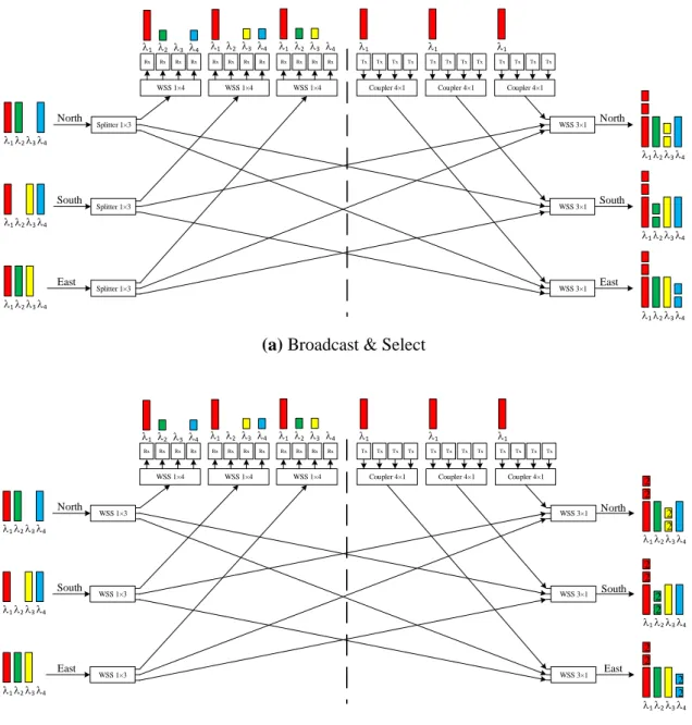
Figure 4.3 - A 3-degree C ROADM implementation based on a (a) B&S and (b) R&S architecture with the crosstalk generation inside this structure. ... 41
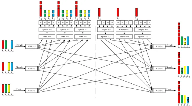
Figure 4.4 - A 3-degree CD ROADM based on a (a) B&S and (b) R&S architecture with the crosstalk generation inside this structure. ... 43 Figure 4.5 - A 3-degree CDC ROADM implemented with MCS 100% contentionless based on a (a) B&S and (b) R&S architecture with the crosstalk generation inside this structure. ... 45 Figure 4.6 - A 3-degree CDC ROADM implemented with WSS 100% contentionless based on a (a) B&S and (b) R&S architecture with the crosstalk generation inside this structure. ... 46 Figure 4.7 - Five-node star network with a full-mesh logical topology. ... 47 Figure 4.8 - A 4-degree (a) C (b) CD (c) CDC implemented with MCS (d) CDC
implemented with WSS ROADM based on a R&S architecture with the crosstalk
generation inside these structures. ... 50 Figure 5.1 - Schematic model of an optical network based on a cascade of ROADMs. 55 Figure 5.2 - Model of a cascade of M multi-degree CDC ROADMs based on the R&S architecture with detail on the in-band crosstalk signals generation. ... 55 Figure 5.3 - Transfer function used to model the (a) optical Super-Gaussian 4th order passband filter 𝐻𝑝(𝑓), optical multiplexer 𝐻𝑀𝑢𝑥(𝑓) and demultiplexer 𝐻𝐷𝑒𝑚𝑢𝑥(𝑓), with
B0 = 41 GHz and (b) optical stopband filters 𝐻𝑏(𝑓) with different blocking amplitudes
(i) 20 dB (ii) 30 dB (iii) 40 dB and (iv) 50 dB and B0 ~ 48 GHz. ... 60
Figure 5.4 - Power spectrum of a 50-Gb/s NRZ QPSK signal for three scenarios: i) signal after passing the optical passband filter 𝐻𝑝(𝑓) (black curve) ii) after passing one
stopband filter 𝐻𝑏(𝑓) with A = 20 dB (blue curve) and iii) after passing one stopband filter 𝐻𝑏(𝑓) with A = 50 dB (red curve). ... 60 Figure 5.5 - Passband narrowing of the optical filter 𝐻𝑝(𝑓) for a 4th Super-Gaussian
filter with B0 equal to 41 GHz after passing through several passband filters. ... 61
Figure 5.6 - (a) 50-Gb/s NRZ QPSK signal power as a function of the optical passband filters that the signal passes (b) Power spectrum of the same signal i) after one filtering (black curve) and ii) after passing through 32 passband filters (red curve). ... 62 Figure 5.7 - Eye diagram of a NRZ QPSK signal after one passband filter (red curve) and after passing through 32 passband filters (black curve). ... 63
xi
Figure 5.8 - (a) 50-Gb/s NRZ QPSK signal power as a function of the number of optical stopband filters that the signal passes. (b) Transfer functions of the cascaded stopband filters for: one filter with A = 40 dB (black curve), two filters each one with
A = 20 dB (red curve) and four filters each one with A = 10 dB (blue curve). ... 64 Figure 5.9 - 50-Gb/s NRZ QPSK power spectrum before (black spectrum) and after passing (a) one stopband filter with A = 40 dB and (b) four stopband filters each one with A = 10 dB (red spectrum). ... 65 Figure 5.10 - Simulation model of the optical network considering one 2×1 WSS. ... 66 Figure 5.11 - BER as a function of the required OSNR for a 25 Gbaud NRZ QPSK (blue line) and 16-QAM (red line) signal using the simulation model presented in figure 5.10 without the crosstalk impairment. ... 66 Figure 5.12 - BER as a function of the required OSNR for one 2×1 WSS with different blocking amplitudes, for 25 Gbaud NRZ (a) QPSK and (b) 16-QAM signals. ... 68 Figure 5.13 - OSNR penalty as a function of the crosstalk level for a single in-band crosstalk signal for QPSK (blue line) and 16-QAM (red line) modulation formats with a symbol rate of 25 Gbaud. ... 69 Figure 5.14 - Simulation model of an add/drop structure based on MCS. ... 70 Figure 5.15 - Simulation model of an add/drop structure based on N×M WSS. ... 70 Figure 5.16 - Crosstalk level as a function of the number of inputs for 20 dB, 30 dB,
40 dB and 50 dB blocking amplitudes considering the add/drop structures based on MCSs or N×M WSSs. ... 71 Figure 5.17 - Simulation model to study the optical filtering effect on an optical
network composed by M cascaded ROADMs. ... 72 Figure 5.18 - BER as a function of the required OSNR for a 50-Gb/s NRZ QPSK signal that passes through a cascade of several ROADMs nodes. ... 73 Figure 5.19 - Simulation model of an optical network composed by M ROADMs
impaired by ASE noise and in-band crosstalk. ... 74 Figure 5.20 - Crosstalk level as a function of the number of ROADM nodes, for a 50-Gb/s NRZ QPSK signal and add/drop structures implemented with MCSs, for
stopband filters with blocking amplitudes of (a) 30 dB and (b) 20 dB. ... 76 Figure 5.21 - Crosstalk level as a function of the number of ROADM nodes, for a 50-Gb/s NRZ QPSK signal and add/drop structures implemented with N×M WSSs, for stopband filters with blocking amplitudes of (a) 30 dB and (b) 20 dB. ... 76
Figure 5.22 - OSNR penalty as a function of the number of ROADMs nodes, for several ROADMs degrees, for a blocking amplitude of 20 dB and with the add/drop structures implemented with (a) MCSs or (b) N×M WSSs. ... 78 Figure 5.23 - Simulation model of a cascade of M multi-degree CDC ROADMs based on the R&S architecture with the in-band crosstalk signals generation and the ASE noise addition. ... 78 Figure 5.24 - Required OSNR as a function of the number of ROADMs for the degrees: 2, 4, 8 and 16, for a network without in-band crosstalk. ... 80 Figure 5.25 - OSNR penalty as a function of the number of ROADMs nodes for a blocking amplitude of 20 dB and with add/drop structures implemented with (a) MCSs or (b) N×M WSSs in a network with amplification at ROADMs inputs and outputs. ... 80 Figure 5.26 - Total signal power as a function of the number of 16-degree CDC
ROADMs nodes with add/drop structures implemented with (a) MCSs or (b) N×M WSSs for the blocking amplitudes of 20 dB and 30 dB. ... 81
xiii
List of Tables
Table 2.1 - QPSK mapping ... 9 Table 2.2 - 16-QAM mapping ... 10 Table 3.1 - Difference between the components used, advantages and disadvantages of the B&S and R&S ROADMs architectures. ... 33 Table 4.1 - Number of in-band crosstalk terms generated inside a N-degree C, CD and CDC ROADM. ... 51 Table 5.1 - B0 and isolation floor bandwidth of the stopband filter as a function of the
blocking amplitude. ... 63 Table 5.2 - Parameters used in the simulator validation. ... 66 Table 5.3 - Parameters used in the simulator to study the physical impairments. ... 72 Table 5.4 - OSNR required for a BER = 103 and the respective OSNR penalty due to
the optical filtering inside the ROADMs nodes. ... 74 Table 5.5 - Crosstalk level at the end of an optical network with 32 CDC ROADMs. . 77
xv
List of Acronyms
ASE Amplified Spontaneous Emission AWG Arrayed-Waveguide Gratings AWGN Additive White Gaussian Noise B&S Broadcast and Select
BER Bit Error Rate
CDC Colorless, Directionless and Contentionless DEC Direct Error Counting
DSP Digital Signal Processing
DWDM Dense Wavelength-Division Multiplexing EDFA Erbium-Doped Fiber Amplifier
FEC Forward Error Correction GF Galois Fields
IP Internet Protocol
IQ In-phase and Quadrature ISI Inter-Symbolic Interference
ITU International Telecommunications Union LCoS Liquid Crystal on Silicon
LO Local Oscillator
MC Monte-Carlo
MCS Multicast Switch
MEMS Micro-Electro-Mechanical Systems M-QAM M-ary Quadrature Amplitude Modulation
NRZ Nonreturn-to-Zero
O/E/O Optic-Electric-Optic conversion OA Optical Amplifier
OADM Optical Add/Drop Multiplexers OSA Optical Spectrum Analyzer OSNR Optical-Signal-to-Noise Ratio OSSM Optical Spatial Switching Matrix OTH Optical Transport Hierarchy
OXC Optical Cross-Connects
PDM Polarization-Division Multiplexing PSD Power Spectrum Density
QPSK Quadrature Phase-Shift Keying R&S Route and Select
ROADM Reconfigurable Optical Add/Drop Multiplexer SDH Synchronous Digital Hierarchy
SONET Synchronous Optical Network WDM Wavelength-Division Multiplexing WSS Wavelength Selective Switch
xvii
List of Symbols
𝐵0 –3 dB bandwidth of the optical filters
𝐴 Blocking amplitude of stopband optical filter
𝑋𝑀,𝑎𝑑𝑑 Crosstalk generated at add section of the Mth ROADM
𝑋𝑀,𝑖𝑛 Crosstalk generated at inputs of the Mth ROADM
𝑋𝑐 Crosstalk level
𝐼𝑝(𝑡) Current produced by the received optical signal 𝐼𝑖(𝑡) Detected signal in-phase component
𝐼𝑞(𝑡) Detected signal quadrature component 𝐸𝑖𝑛(𝑡) Electrical field incident on the photodetector 𝛿𝑋𝑇 In-band crosstalk penalty
𝐸𝐿𝑂(𝑡) Local oscillator electric field
𝑃𝐿𝑂 Local oscillator power
𝑁𝑒 Number of counted bits errors
𝑁𝑀𝐶 Number of generated sample functions
𝑀 Number of ROADMs cascade
𝑁𝑎 Number of samples per symbol 𝑁𝑠 Number of simulated symbols
𝑁𝑏 Number of transmitted bits 𝛿𝐹 Optical filtering penalty 𝑅𝑥 Optical receiver
𝐵𝑂𝑆𝐴 Optical spectrum analyzer bandwidth
𝑅𝑥 Optical transmitter
𝑆𝑜,𝑀 Output optical signal of the Mth ROADM
𝑅𝜆 Photodetector responsivity 𝑃𝑖𝑛 Power of the amplified signal
𝑃𝐴𝑆𝐸 Power of the ASE noise
𝑃𝑥 Power of the interfering signals 𝑃0 Power of the primary signal 𝑁𝐴𝑆𝐸 PSD of ASE noise
𝑆𝑖𝑛,𝑓(𝑓) PSD of the filtered primary optical signal 𝑆𝑖𝑛(𝑓) PSD of the primary optical signal
𝑆𝑜𝑢𝑡(𝑓) PSD of the signal at the optical receiver input 𝑃𝑖𝑛(𝑡) Received optical power
𝐸𝑟(𝑡) Received signal electric field
𝑁 ROADM degree
𝐵𝑠𝑖𝑚 Simulation bandwidth
𝐻𝐷𝑒𝑚𝑢𝑥(𝑓) Transfer function of optical demultiplexer
𝐻𝑀𝑢𝑥(𝑓) Transfer function of optical multiplexer 𝐻𝑝(𝑓) Transfer function of optical passband filter 𝐻𝑏(𝑓) Transfer function of optical stopband filter
1
Chapter 1
Introduction
The exponential growth of internet data traffic due to the increase of the number of devices (millions of connected devices are expected in the coming years), cloud services (lots of network functionalities are being put in the cloud) or video-on-demand [1], have been putting fiber optic network technologies in a continuous development in order to be able to support all the data traffic generated. Technologies, such as dense wavelength-division multiplexing (DWDM) [2], flexible grid [3], high order modulation formats [4], coherent detection and advanced digital signal processing techniques (DSP) [5] are now fundamental and mandatory to achieve the huge transport capacities required by the overall telecommunications infrastructure.
In addition to these technologies, the evolution of the optical network nodes is also very important to support this growth. In the past, these nodes were static and manual configuration was needed, nowadays, with the technology evolution, these nodes are becoming more reconfigurable [6]. This reconfigurability improves the routing and switching functionalities in the optical nodes, making them faster, dynamic and more reliable. Currently, these optical nodes are implemented with reconfigurable optical add/drop multiplexers (ROADMs).
On the other hand, the optical network physical layer limitations require a deeper study because the optical signal along its light-path, passes through optical fiber links as well as many network components inside the ROADMs, such as optical switches, (de)multiplexers or splitters/couplers. Consequently, the losses, noises and interferences accumulated along the light-path will degrade the optical signal transmission along the optical network. One of the optical network physical layer impairments that becomes enhanced along the optical signal light-path and degrades the optical network performance is the in-band crosstalk [7].
CHAPTER 1. INTRODUCTION
1.1 Road to Flexible Optical Networks Based on ROADMs
Fiber optics communications continue to evolve in order to support all the traffic that is being thrown to the network. Most of this traffic is, nowadays, based on the Internet Protocol (IP) which requires an optical network more flexible and dynamic [6].
The growing traffic demand leads also to the need of higher bit rates per optical channel. The well-known fixed grid, with an optical channel spacing of 50 GHz, even with sophisticated modulation schemes, no longer works for 400 Gb/s and above. Therefore, many efforts have been made to standardize a new grid, the flexible grid [3]. In this scenario, the optical channel spacing can be adjusted accordingly to the network needs, leading to optical channels with a larger space and high granularity, consequently, they are able to carry higher bit rates than with a fixed grid. Currently, the international telecommunication union (ITU) recommends a grid granularity of 6.25 GHz with a minimum frequency slot of 12.5 GHz [8], [9]. For example, we can have an optical channel with 37.5 GHz or 75 GHz instead of the most commons with 50 GHz and 100 GHz spacings. Recent studies demonstrated that a grid granularity of 6.25 GHz gives more freedom to adjust the spacing between the optical channels and avoid portions of unused spectrum [10], [11].
Consequently, given the change of traffic type and the implementation of a more flexible optical network, the ROADM nodes and all optical network components must be developed with new characteristics. In the ROADM nodes, the main changes are found in the add/drop structures, with the implementation of the colorless, directionless and contentionless features [6].
1.2 Coherent Detection and Modulation Formats
One of the techniques that leads to a great improvement of the optical networks performance is the coherent detection alongside with advanced DSP. Systems with coherent detection allow that the information carried in the optical signal can be coded in amplitude, frequency, phase and polarization, allowing the use of higher modulation formats. Furthermore, with coherent detection, polarization-division multiplexing (PDM) is typically used [12], [13]. The PDM technique allows transmitting two modulated
CHAPTER 1. INTRODUCTION
3
Another advantage of coherent detection is the possibility of using advanced DSP hardware at the optical receivers to compensate any linear impairments occurring during transmission [14]. Linear impairments, such as the chromatic and polarization mode dispersions, are compensated by the DSPs and this compensation is fundamental to achieve such high data rates. Some of the non-linear impairments can be also compensated with the use of DSPs [14]. On the other hand, coherent detection requires optical receiver structures more complex and expensive than in direct detection receivers. In 2010, the optical coherent receivers were commercial available and the optical channel capacity increased to 100 Gb/s with the use of advanced modulation formats, such as the quadrature phase-shift keying (QPSK), in addition to PDM and advanced DSPs [15].
In the future, and possibly with the introduction of the flexible grid and the superchannel concept, the optical channel capacity will go to 400 Gb/s and 1 Tb/s, using higher order modulation formats than the QPSK, such as PDM-8 quadrature amplitude modulation (QAM) and PDM-16-QAM [16], [17].
1.3 In-Band Crosstalk
The crosstalk is a physical layer impairment which is mainly caused by the imperfect isolation of the optical components inside a ROADM node [7]. The imperfect isolation leads to optical signal leakages that are added to the desired (primary) signal along the light-path and lead to system performance degradation. The in-band crosstalk is worse than other types or crosstalk, such as out-of-band crosstalk, for the network performance since it cannot be removed by optical filtering at the receiver [18]. It occurs when the interfering signals have the same nominal wavelength as the desired signal, but are originated from different laser sources. In-band crosstalk can lead to a serious network performance degradation [7].
In an optical network based on ROADMs, the in-band crosstalk will accumulate over the ROADM cascade and can limit the number of nodes that the signal pass in the network [19]. In this work, our main focus is to study exhaustively the impact of in-band crosstalk generated inside of ROADMs nodes on the network performance. This study is performed by properly modeling the ROADM node, with different architectures and add/drop structures types, and the in-band crosstalk generated inside them.
CHAPTER 1. INTRODUCTION
In the literature, some studies were performed to address the impact of the in-band crosstalk due to cascaded ROADMs on the network performance, however with a simple ROADM model [20] or not considering the add/drop structures [21]. In this work, we model more rigorously the multi-degree colorless, directionless and contentionless (CDC) ROADMs considering the ROADM components: type of add/drop structures and respective architectures.
1.4 Dissertation Organization
This dissertation is organized as follows. In Chapter 2, we describe how we simulate the optical communication network to transmit and receive M-QAM signals, explaining the important aspects of this implementation and the modeling of the optical components. The third chapter focuses on the study of the ROADMs nodes and its components. A summary about the evolution, main characteristics and architectures of the ROADMs is presented. We discuss the properties of ROADM add/drop structures, namely CDC structures. The advantages and disadvantages of ROADMs broadcast and select (B&S) and route and select (R&S) architectures are also discussed in this chapter.
In the fourth chapter, the crosstalk generated inside the ROADMs nodes is studied considering a start topology network with 4 and 5 ROADMs. The number of in-band crosstalk terms that are generated inside a multi-degree CDC ROADM is quantified.
In the fifth chapter, the performance of an optical network impaired by in-band crosstalk, optical filtering and amplified spontaneous emission
(
ASE) noise based on CDC ROADMs, implemented with multicast switches (MCSs) and wavelength selective switches (WSSs), is evaluated. The network simulation model is presented as well as the in-band crosstalk signals generated through the optical signal path.Finally, the sixth chapter summarizes the main conclusions of this dissertation and provides some ideas for possible future work.
CHAPTER 1. INTRODUCTION
5
1.5 Dissertation Main Contributions
The main contributions of this work to the research topics studied are the following: 1. CDC ROADM model, for B&S and R&S architectures, that takes into account the in-band crosstalk generated inside these nodes. Two add/drop structures were considered, MCS-based and WSS-based;
2. Assessment of the impact of the in-band crosstalk, optical filtering and ASE noise in an optical network composed by multi-degree CDC ROADMs, considering QPSK signals and assuming a fixed grid.
References
[1] Cisco Systems, “Cisco Visual Networking Index: Forecast and methodology, 2016-2021,” White Paper. San Jose, CA, USA, 2016.
[2] J. Kahn and K. Ho, "Spectral efficiency limits and modulation/detection techniques for DWDM systems," in IEEE Journal of Selected Topics in Quantum Electronics, vol. 10, no. 2, pp. 259-272, April 2004.
[3] O. Gerstel, M. Jinno, A. Lord and S. Yoo, "Elastic optical networking: a new dawn for the optical layer?," in IEEE Communications Magazine, vol. 50, no. 2, pp. s12-s20, February 2012.
[4] P. Winzer, "High-Spectral-Efficiency Optical Modulation Formats," in Journal of
Lightwave Technology, vol. 30, no. 24, pp. 3824-3835, December 2012.
[5] E. Ip, A. Lau, D. Barros, and J. Kahn, “Coherent detection in optical fiber systems,”
Optics Express, vol. 16, no. 2, pp. 753–791, January 2008.
[6] S. Gringeri, B. Basch, V. Shukla, R. Egorov and T. Xia, "Flexible architectures for optical transport nodes and networks," in IEEE Communications Magazine, vol. 48, no. 7, pp. 40-50, July 2010.
[7] I. Monroy and E. Tangdiongga, Crosstalk in WDM Communication Networks. Norwell, MA: Springer, 2002.
[8] “Spectral Grids for WDM Applications: DWDM Frequency Grid,” ITU-T Recommendation G.694.1, 2012 [Online].
Available: https://www.itu.int/rec/T‑REC‑G.694.1/en.
[9] M. Jinno, "Elastic Optical Networking: Roles and Benefits in Beyond 100-Gb/s Era," in Journal of Lightwave Technology, vol. 35, no. 5, pp. 1116-1124, March 2017.
[10] D. Xie et al., "LCoS-Based Wavelength-Selective Switch for Future Finer-Grid Elastic Optical Networks Capable of All-Optical Wavelength Conversion," in IEEE
Photonics Journal, vol. 9, no. 2, pp. 1-12, April 2017.
[11]J. Pedro, "Designing transparent flexible-grid optical networks for maximum spectral efficiency [Invited]," in IEEE/OSA Journal of Optical Communications and Networking, vol. 9, no. 4, pp. C35-C44, April 2017.
[12] C. Fludger et al., "Coherent Equalization and POLMUX-RZ-DQPSK for Robust 100-GE Transmission," in Journal of Lightwave Technology, vol. 26, no. 1, pp. 64-72, January 2008.
CHAPTER 1. INTRODUCTION
[13] P. Winzer, A. Gnauck, C. Doerr, M. Magarini and L. Buhl, "Spectrally Efficient Long-Haul Optical Networking Using 112-Gb/s Polarization-Multiplexed 16-QAM," in Journal of Lightwave Technology, vol. 28, no. 4, pp. 547-556, February 2010.
[14]J. Zhang, J. Yu and H. Chien, "Linear and Nonlinear Compensation for 8-QAM SC-400G Long-Haul Transmission System," in Journal of Lightwave Technology, vol. PP, no. 99, pp. 1-1, September 2017.
[15] L. Nelson et al., "WDM performance and multiple-path interference tolerance of a real-time 120 Gbps Pol-Mux QPSK transceiver with soft decision FEC," 2012 Optical
Fiber Communication Conference and Exposition and the National Fiber Optic Engineers Conference (OFC/NFOEC), Los Angeles, CA, 2012, pp. 1-3, March 2012.
[16] P. Winzer, "Beyond 100G Ethernet," in IEEE Communications Magazine, vol. 48, no. 7, pp. 26-30, July 2010.
[17] P. Winzer, “Scaling optical fiber networks: Challenges and solutions.” Optics and
Photonics News, vol. 26, no. 3, pp. 28-35, March 2015.
[18] P. Legg, M. Tur and I. Andonovic, "Solution paths to limit interferometric noise induced performance degradation in ASK/direct detection lightwave networks," in Journal of Lightwave Technology, vol. 14, no. 9, pp. 1943-1954, September 1996. [19] S. Tibuleac and M. Filer, "Transmission Impairments in DWDM Networks With Reconfigurable Optical Add-Drop Multiplexers," in Journal of Lightwave Technology, vol. 28, no. 4, pp. 557-598, February 2010.
[20] M. Filer and S. Tibuleac, "Generalized weighted crosstalk for DWDM systems with cascaded wavelength-selective switches," 2012 Conference on Optical Fiber
Communication and the National Fiber Optic Engineers Conference (OFC/NFOEC),
Los Angeles, CA, pp. 1-3, March 2012.
[21] M. Filer and S. Tibuleac, "N-degree ROADM architecture comparison: Broadcast-and-select versus route-Broadcast-and-select in 120 Gb/s DP-QPSK transmission systems," 2014
Optical Fiber Communication Conference and Exhibitions (OFC), San Francisco, CA,
7
Chapter 2
Simulation Model of an Optical Communication
Network
2.1 Introduction
In this chapter, a generic simulation model of an optical communication network is presented, and some important aspects for its implementation using computer simulation are described.
In section 2.2, we explain with some detail the existing optical components in an optical network and how they are modeled in the Matlab software. The optical transmitter and its main characteristics are presented in subsection 2.2.1. The signal modulation formats studied in this dissertation are also presented. The power spectrum density (PSD) functions, constellations and eye diagrams obtained by simulation are shown for QPSK and 16-QAM modulation formats. Subsection 2.2.2 is reserved for presenting the optical fiber. In subsection 2.2.3, the optical coherent receiver structure is presented and explained. The optical amplifier is characterized in subsection 2.2.4.
The Monte Carlo (MC) simulator developed to assess the performance of the optical communication networks described in previous section, and implemented in Matlab, is described by a flow-chart in section 2.3.
In section 2.4, the metrics used in this work to evaluate the performance of an optical communication network using MC simulation, the direct error counting (DEC) and optical-signal-to-noise ratio (OSNR) penalty, are presented.
CHAPTER 2. SIMULATION MODEL OF AN OPTICAL COMMUNICATION NETWORK
2.2 Generic Model of the Optical Network
In this section, a generic simulation model of an optical communication network is presented and explained, as well as four of its main components: the optical transmitter, the optical fiber, the optical coherent receiver and the optical amplifier. As in this work the focus is about the impairments in the optical nodes, we reserve chapters 3 and 4 to present all characteristics and technological evolution of the ROADMs network nodes.
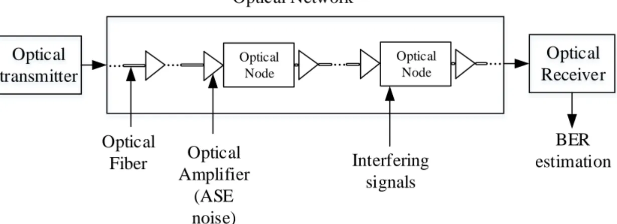
Figure 2.1 depicts a generic simulation model of the optical communication network. The optical signals are generated by an optical transmitter, which will be described in subsection 2.2.1. Subsequently, the transmitted signal enters the optical network, it passes through the optical links (which are composed by the optical fiber, optical amplifiers and optical nodes) until it reaches the optical receiver. The characteristics of the optical fiber are described in subsection 2.2.2 and the model considered for the amplifiers is described in subsection 2.2.4. Along its optical path in the network, ASE noise from amplification and the interfering signals from imperfect isolation of the optical components inside the nodes are generated and added to desired (primary) signal. At the optical network output, the signal impaired by ASE noise and interfering signals reaches the optical receiver. In this work, we consider a coherent detection receiver, which will be described with detail in subsection 2.2.3. When the signal is detected in the optical receiver, the optical network performance is evaluated through the bit error rate (BER) estimation.
Optical transmitter Optical Receiver BER estimation Optical Network ... Optical Node Optical Amplifier (ASE noise) Optical Node ... ... ... Optical Fiber Interfering signals
CHAPTER 2. SIMULATION MODEL OF AN OPTICAL COMMUNICATION NETWORK
9
2.2.1 Optical Transmitter
Regarding the data sequence, in computer simulations, it is important to choose a suitable symbols sequence for obtaining reliable results. Typically, pseudo-random binary sequences are used to represent the data sequence [1]. Since in this work, we simulate M-QAM signals (QPSK/4-QAM and 16-QAM), the symbols sequence was generated using Galois Fields (GF) arithmetic [1]. In our simulations, this method produces a sequence of 256 symbols for QPSK signals and of 512 symbols for 16-QAM signals. These sequences lengths are chosen to take into account accurately the effect of inter-symbolic interference (ISI) on the signal.
In Matlab software, the symbols sequences are represented by discrete vectors in the time or in the frequency domains. The time vector has NsNa positions, where Ns is the
number of simulated symbols and Na is the number of samples per symbol. We assume
Na = 64 which gives us a good definition of the sequence generated. The frequency vector,
which has the same number of positions as the time vector, is obtained by computing the
Fast Fourier Transform of the time vector.
After generating the symbols sequence, the next step performed is the mapping. The main function of the mapping is to assign amplitude levels corresponding to the in-phase and quadrature components of the input sequence of symbols. Generally, the generation of an optical signal in an optical communication network is accomplished using a laser followed by an in-phase/quadrature (IQ) modulator [2]. In this work, we assume an ideal
optical transmitter. Tables 2.1 and 2.2 represent the mapping used for QPSK and 16-QAM signals, respectively, where a Gray mapping is assumed. The constellations for
these modulation formats at the optical transmitter output are shown in figure 2.2. The bits represented in both figures correspond to the mapping shown in Tables 2.1 and 2.2.
Table 2.1 - QPSK mapping Symbol Bits Symbol mapped
1 00 1j
2 01 1+j
3 11 1+j
CHAPTER 2. SIMULATION MODEL OF AN OPTICAL COMMUNICATION NETWORK
Table 2.2 - 16-QAM mapping
Symbol Bits Symbol mapped Symbol Bits Symbol mapped
1 0000 33j 9 1000 33j 2 0001 3j 10 1001 3j 3 0010 3+3j 11 1010 3+3j 4 0011 3+j 12 1011 3+j 5 0100 13j 13 1100 13j 6 0101 1j 14 1101 1j 7 0110 1+3j 15 1110 1+3j 8 0111 1+j 16 1111 1+j (a) (b)
Figure 2.2 - Constellations for (a) QPSK and (b) 16-QAM modulation formats with the respective mappings.
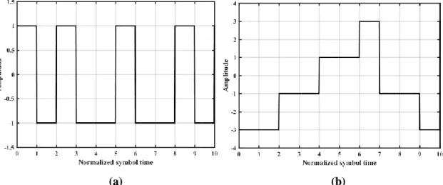
The focus of this work is mainly on the QPSK modulation format, since it is the most common modulation format, in links with 100-Gb/s data rates and coherent detection. Although, we also present some studies regarding the 16-QAM modulation format. For example, in chapter 5, the validation of our simulation model will be made for both modulation formats. In the following, we present the optical signals and PSDs obtained for both modulation formats, QPSK and 16-QAM, at the output of the optical transmitter. In this work, we generate the optical signals with rectangular shape and with a bit rate of 50-Gb/s. This bit rate corresponds to a single polarization of the optical signal. Figure 2.3 shows a sequence of rectangular pulses for a nonreturn-to-zero (NRZ) QPSK signal, figure 2.3 (a), and for a NRZ 16-QAM signal, figure 2.3 (b).
CHAPTER 2. SIMULATION MODEL OF AN OPTICAL COMMUNICATION NETWORK
11
Figure 2.4 depicts the PSD of a 50-Gb/s NRZ rectangular (a) QPSK and (b) 16-QAM signals. By observing this figure, for the QPSK modulation format (Figure 2.4 (a)) the bandwidth of the main lobe is 50 GHz, while for 16-QAM (Figure 2.4 (b)) is 25 GHz.
(a) (b)
Figure 2.3 - (a) QPSK and (b) 16-QAM signals generated with rectangular pulses.
(a) (b)
Figure 2.4 - PSDs of a 50-Gb/s NRZ rectangular (a) QPSK and (b) 16-QAM signals.
Notice that the interfering signals, which arise along the optical network are assume as being generated by identical optical transmitters. Throughout this work, we assume always that the interfering signals have the same attributes as the transmitted signal: same modulation format, baud rate, and OSNR level, but with arbitrary different transmitted symbols, different phase and with a time misalignment between the desired signal and the interfering signal. The phase difference is modeled as a uniform distributed random variable between 0 and 2π. The time misalignment is modeled as a uniform distributed random variable between 0 and the symbol time [3].
CHAPTER 2. SIMULATION MODEL OF AN OPTICAL COMMUNICATION NETWORK
2.2.2 Optical Fiber
Another important component of the optical network is the optical fiber. Besides other advantages, the optical fiber extremely large bandwidth and low attenuation, about 0.2 dB/km, allows very high capacity transmission with very long reach. Hence, optical fiber is the selected guided media that supports the overall telecommunications infrastructure and its increasing demand for data traffic. It is responsible for carrying the optical signal along the optical network.
However, the optical fiber introduces impairments that degrade the transmission performance: attenuation, dispersion and fiber nonlinearities [4]. The optical signal attenuation can be compensated by the optical amplification in the network. The optical dispersion, either chromatic dispersion or polarization mode dispersion, are nowadays compensated by the DSPs present in the coherent detectors [5]. The optical fiber nonlinearities occur for high launched powers at the fiber input, and its effect is reduced in presence of high accumulated dispersion along the optical network. Furthermore, the DSPs of the coherent receiver can also compensate some of the nonlinearities impact [6]. In this work, the main focus is to study the impact of the in-band crosstalk in the optical network. As other effects that impair the optical signal can mask the impact of the in-band crosstalk on the network performance, we assume an ideal fiber transmission in an optical network simulation model, and neglect the optical fiber impairments.
2.2.3 Optical Coherent Receiver
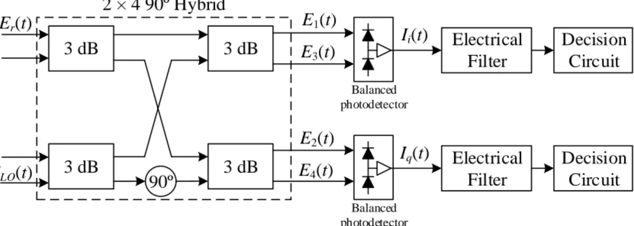
In this subsection, the model used for the optical coherent receiver is described. As we mentioned in the previous chapter, the coherent detection is nowadays the most used detection technology in long-haul networks with high capacity per optical channel (100-Gb/s and above). Figure 2.5 depicts the block diagram of the optical coherent receiver for a single polarization of the signal, as considered in this work. Since, in this work we assume that these components are ideal, the receiver performance can be assessed considering only the structure of figure 2.5 for a single polarization of the signal [7]. The coherent receiver with dual polarization consists of two polarization beam splitters connected with two structures identical to the one depicted in figure 2.5.
CHAPTER 2. SIMULATION MODEL OF AN OPTICAL COMMUNICATION NETWORK
13
The structure of the optical coherent receiver is formed by a 2×4 90º hybrid followed by two balanced photodetectors. There are many possibilities for implementation of the hybrid. We have chosen the most commonly and commercially available implementation. The hybrid, shown in figure 2.5, is composed by four 3 dB couplers and a 90º phase shift in the lower branch, which allows the receiver to decode the in-phase and quadrature signal components of the received current, 𝐼𝑖(𝑡) and 𝐼𝑞(𝑡), respectively.
3 dB Er(t) 3 dB 3 dB 3 dB ELO(t) E1(t) E3(t) E2(t) E4(t) 2 × 4 90º Hybrid Balanced photodetector Balanced photodetector Iq(t) Ii(t) 90º Electrical Filter Electrical Filter Decision Circuit Decision Circuit
Figure 2.5 - Block diagram of the model used for the optical coherent receiver for a single polarization of the signal.
In figure 2.5 𝐸𝑟(𝑡) and 𝐸𝐿𝑂(𝑡) denote the complex envelope of received signal (at
the output of the optical network) and local oscillator (LO) field. The 2×4 90º Hybrid is described by the following input/output relationship [7]
[ 𝐸1(𝑡) 𝐸2(𝑡) 𝐸3(𝑡) 𝐸4(𝑡)] = 1 2 . [ 1 1 1 𝑗 1 − 1 1 − 𝑗 ] . [𝐸𝑟(𝑡) 𝐸𝐿𝑂(𝑡)] (2.1)
The LO is an essential component of a coherent receiver. It allows the coherent receiver to decode the signal information in both in-phase and quadrature components. To maximize the coherent receiver performance, the LO frequency must be as close as possible to the optical carrier frequency [8]. In this work, the LO is considered synchronized with the optical carrier frequency and noises generated in this component are neglected. Hence, the LO can be defined as 𝐸𝐿𝑂 = √𝑃𝐿𝑂, where 𝑃𝐿𝑂 is the power of
CHAPTER 2. SIMULATION MODEL OF AN OPTICAL COMMUNICATION NETWORK
Each balanced photodetector, depicted in figure 2.5, converts the optical signal to an electrical signal. The operation of a photodetector can be described by its responsivity defined by [9]
𝑅𝜆 = 𝐼𝑝(𝑡)
𝑃𝑖𝑛(𝑡) (2.2)
where 𝐼𝑝(𝑡) is the current produced at the output of the photodetector by the incident optical power 𝑃𝑖𝑛(𝑡) at the photodetector input. In this work, for simplification, we will
consider that the photodetector responsivity is 𝑅𝜆 = 1 [A/W]. Hence 𝑃𝑖𝑛(𝑡) = |𝐸𝑖𝑛(𝑡)|2,
where 𝐸𝑖𝑛(𝑡) is the electrical field incident on the photodetector.
All optical receivers have a low pass filter after the photodetection and before the decision circuit, as represented in figure 2.5, to reduce the ISI and the noise, consequently improve the OSNR [10]. Ideally, the shape of this filter must be the same of the incoming signal. Theses filters are known as matched filters [11]. In this work, we used a 5th order Bessel filter as the received electrical filter, which is a typical model used in several studies [12], [13]. The 3 dB bandwidth of this electrical filter is equal to the symbol rate. Figure 2.6 illustrates the eye diagrams of a received electrical signal without physical impairments for both modulation formats, QPSK and 16-QAM. As we can see by these figures, at the optical receiver, after passing through the 5th order Bessel electrical filter, the eye diagrams are completely open at the optimum sampling time instant.
(a) (b)
Figure 2.6 - Eye diagrams of a received electrical signal without physical impairments for (a) QPSK and (b) 16-QAM modulation formats.
CHAPTER 2. SIMULATION MODEL OF AN OPTICAL COMMUNICATION NETWORK
15
2.2.4 Optical Amplifier
In an optical network, the optical signal suffers attenuation which is introduced mainly by the optical fiber, but also by the several components that the signal passes until it reaches its destination. To compensate the path losses, in-line optical amplification is essential [9]. In addition to in-line amplification, i.e., between the optical fibers links, normally, we find optical amplifiers (OA) also at all ROADM inputs/outputs [14]. The optical amplification in the ROADMs inputs is mainly to compensate the path losses, while in the ROADMs outputs is to compensate the power losses inside the nodes.
There are three main types of OA: Erbium-Doped Fiber Amplifiers (EDFAs), semiconductor optical amplifiers and Raman Amplifiers. The most commonly used in the optical nodes and the one considered in this work is the EDFA. This type of OA can achieve a high gain, about 30 dB, and operates in the C band (1530 – 1565 nm), the band commonly used in optical communications [15].
However, optical amplification also adds ASE noise to the signal, which degrades the system performance [9]. In this work, we assume that the AOs compensate exactly the network losses, and only add ASE noise to the signal. The ASE noise power is defined by setting the OSNR, which can be defined by
𝑂𝑆𝑁𝑅 = 𝑃𝑖𝑛
𝑃𝐴𝑆𝐸 (2.3)
where 𝑃𝑖𝑛 is the average power of the signal at the OA output, and the 𝑃𝐴𝑆𝐸 is the average
power of the ASE noise added to the signal by the OA, which is defined by
𝑃𝐴𝑆𝐸= 𝑁𝐴𝑆𝐸𝐵𝑂𝑆𝐴 (2.4)
where 𝐵𝑂𝑆𝐴 is the optical spectrum analyzer (OSA) bandwidth with the typical value of 12.5 GHz and is related to the simulation bandwidth 𝐵𝑠𝑖𝑚 by [16]
𝐵𝑂𝑆𝐴 = 𝐵𝑠𝑖𝑚𝑁𝐴𝑆𝐸
𝑃𝐴𝑆𝐸 (2.5)
In equations 2.4 and 2.5, the 𝑁𝐴𝑆𝐸 is the PSD of the generated ASE noise. In this work, the ASE noise is considered to be an Additive White Gaussian Noise (AWGN).
CHAPTER 2. SIMULATION MODEL OF AN OPTICAL COMMUNICATION NETWORK
2.3 Monte-Carlo Simulation Flow-Chart
In this section, we explain the MC simulation with the support of the flow-chart depicted in figure 2.7 [17]. The flow-chart represents the simulator implemented in the Matlab software to evaluate the performance of the optical communication network that will be studied in this work. The MC method is a well-known technique for statistical simulation in several scientific areas, where there is the need to describe and characterize the influence of a stochastic process in a specific system.
The flow-chart in figure 2.7 works as follow. The first iteration of the MC simulation is to save the reference signal (the transmitted signal), without the addition of any statistical sample function. With this reference signal, the receiver knows the transmitted symbols, can obtain the propagation delay of the optical network and also the optimum sampling time from the eye diagram of the received signal. From the propagation delay, we can perform exactly the synchronism between the received (impaired by any statistical effect) and transmitted signals.
On the following MC iterations, the statistical sample functions are added to the signal transmitted along the simulated optical communication network. The received signal is compared with the reference signal to check if the received signal has errors. This process is known as DEC. When a specific number of errors is achieved, the MC simulator stops and the BER is estimated.
The main cause of errors in our network simulation model will be the ASE noise and the interfering in-band signals that are generated along the optical network. The statistical sample functions generated in the simulator correspond to those two impairments. In this work, the stopping criteria is considered for a total of 1000 symbols errors in all MC iterations [17].
CHAPTER 2. SIMULATION MODEL OF AN OPTICAL COMMUNICATION NETWORK 17 Start Ideal transmitter 1st iteration? no Optical network yes Save reference signal Receiver Obtain delay and the optimum time sampling Synchronism and signal sampling Comparison with reference signal Stopping criteria is achieved? yes BER estimation End Addition of statistical sample functions
Figure 2.7 - Flow-chart of the MC simulation to obtain the BER of the optical communication network.
2.4 Performance Evaluation Methods
In this work, we use the most common metric for the performance evaluation of optical communication systems, the BER, which is estimated by DEC. The BER is essentially the ratio between the number of bits errors and the total number of transmitted bits. By assuming Gray mapping, the BER is defined by [1], [17]
𝐵𝐸𝑅 = 𝑁𝑒
𝑁𝑀𝐶𝑁𝑏(𝑙𝑜𝑔2𝑀) (2.7)
where Ne is the number of counted bit errors, NMC is the number of generated sample
functions, Nb is the number of transmitted bits in one MC iteration and M is the
modulation order format. In this work, we evaluate the system performance for a BER equal to 103, because after the use of the forward error correction (FEC), the optical
CHAPTER 2. SIMULATION MODEL OF AN OPTICAL COMMUNICATION NETWORK
communication systems can achieve a lower BER, in the order of the 1015 [18]. In typical optical receivers with coherent detection, FEC techniques are implemented in the DSPs.
Another metric used in this work to evaluate the performance of the optical communication systems is the OSNR penalty. It consists of measuring the required OSNR at a desired BER, of the optical network without a specific impairment and then add the desired impairment to the optical network and obtain the required OSNR with that impairment. From the difference between the required OSNRs with and without impairments, the OSNR penalty due to that physical impairment can be estimated. This technique can be applied to the several impairments in an optical network. In this study, we will evaluate the OSNR penalty at a BER of 103, due to the in-band crosstalk, the optical filtering and the ASE noise.
2.5 Conclusions
In this chapter, a generic model of an optical communication network has been described, and the model used in Matlab software to simulate the optical network has also been presented.
We presented with more detail several optical components and their simulation model: the optical transmitter, the optical fiber, the optical coherent receiver, the optical amplifier and the respective modulation formats generated, the QPSK and 16-QAM.
Finally, the MC simulation has been explained through the use of a flow-chart, and the performance evaluation methods of the optical communication network, the BER, estimated by DEC, and the OSNR penalty have been also presented.
CHAPTER 2. SIMULATION MODEL OF AN OPTICAL COMMUNICATION NETWORK
19
References
[1] M. Jeruchim, P. Balaban, and K. Shanmugan, Simulation of Communication Systems:
Modeling, Methodology, and Techniques, 2nd ed. New York: Kluwer, 2000.
[2] G. Agrawal, Lightwave Technology: Telecommunication Systems. New York: Wiley, 2005.
[3] L. Cancela, D. Sequeira, B. Pinheiro, J. Rebola and J. Pires, "Analytical tools for evaluating the impact of in-band crosstalk in DP-QPSK signals," 2016 21st European
Conference on Networks and Optical Communications (NOC), Lisbon, pp. 6-11, June
2016.
[4] A. Chraplyvy, "Limitations on lightwave communications imposed by optical-fiber nonlinearities," in Journal of Lightwave Technology, vol. 8, no. 10, pp. 1548-1557, October 1990.
[5] E. M. Ip and J. M. Kahn, "Fiber Impairment Compensation Using Coherent Detection and Digital Signal Processing," in Journal of Lightwave Technology, vol. 28, no. 4, pp. 502-519, February 2010.
[6] X. Zhou and C. Xie, Enabling Technologies High Spectral-efficiency Coherent
Optical Communication Networks. New Jersey: John Wiley & Sons, 2016.
[7] M. Seimetz and C. Weinert, "Options, Feasibility, and Availability of 2 × 4 90o Hybrids for Coherent Optical Systems," in Journal of Lightwave Technology, vol. 24, no. 3, pp. 1317-1322, March 2006.
[8] L. Binh, Digital processing: optical transmission and coherent receiving techniques. Taylor and Francis, 2013.
[9] G. Agrawal, Fiber-Optic Communication Systems, 4th ed., New York: Wiley, 2010. [10] M. Seimetz, High-Order Modulations for Optical Fiber Transmission, T. Rhodes, Ed. Atlanta, GA:Springer, 2009.
[11] J. Proakis and M. Salehi, Digital Communications, 5th ed. McGraw-Hill, 2008. [12] S. Yao, S. Fu, H. Wang, M. Tang, P. Shum and D. Liu, "Performance comparison for NRZ, RZ, and CSRZ modulation formats in RS-DBS Nyquist WDM system," in IEEE/OSA Journal of Optical Communications and Networking, vol. 6, no. 4, pp. 355-361, April 2014.
[13] G. Bosco, V. Curri, A. Carena, P. Poggiolini and F. Forghieri, "On the Performance of Nyquist-WDM Terabit Superchannels Based on PM-BPSK, PM-QPSK, PM-8QAM or PM-16QAM Subcarriers," in Journal of Lightwave Technology, vol. 29, no. 1, pp. 53-61, January 2011.
[14] T. Zami, "Current and future flexible wavelength routing cross-connects," in Bell
Labs Technical Journal, vol. 18, no. 3, pp. 23-38, December 2013.
[15] R. Ramaswami, K. Sivarajan, and G. Sasaki, Optical Networks: A Practical
Perspective, 3rd ed. San Francisco, CA: Morgan Kaufmann, 2009.
[16] R. Hui and M. O’Sullivan, Fiber Optic Measurement Techniques. Burlington, MA:
Academic, 2009
[17] B. Pinheiro, "Impact of In-Band Crosstalk on the Performance of Optical Coherent Detection Communication Systems", Dissertation presented for the Masters Degree on Telecommunications and Information Science, ISCTE-IUL, 2015.
[18] F. Chang, K. Onohara and T. Mizuochi, "Forward error correction for 100 G transport networks," in IEEE Communications Magazine, vol. 48, no. 3, pp. S48-S55, March 2010.
21
Chapter 3
ROADMs – Evolution, Characteristics, Components
and Architectures
3.1 Introduction
In this chapter, we present the optical network nodes, currently known as ROADMs. In section 3.2, a summary about the ROADMs evolution is presented, since the first generation until the current generation mainly based on WSSs.
Section 3.3 presents the main ROADM characteristics. In section 3.4, the ROADM components are presented.
Next, in section 3.5, the properties and implementation of the ROADM add/drop structures are explained.
In section 3.6 the ROADMs architectures are presented and, its advantages and disadvantages are discussed.
Finally, in section 3.7, the conclusions of this chapter are presented.
3.2 Evolution of ROADMs
When the wavelength division multiplexing (WDM) technology was introduced in the 90’s into transport networks, synchronous digital hierarchy (SDH) network and synchronous optical network (SONET), its main function was to increase the network capacity. The WDM technology was implemented in these networks, mainly in networks with ring topology, as point-to-point connections between the nodes where all the wavelengths were multiplexed/demultiplexed [1]. Consequently, in these first WDM networks, the signal transmission was done at the optical domain and the signal processing (routing and switching) was done in the electrical domain, i.e., there was O/E/O conversion of the signals in the network nodes, as depicted in figure 3.1. These networks are called opaque networks [2]. Opaque networks started having limitations in both the signal processing time and bit rate. Since then, there has been a great evolution in the type and amount of traffic handled by these networks. The traffic type changed
CHAPTER 3. ROADMS – EVOLUTION, CHARACTERISTICS, COMPONENTS AND ARCHITECTURES
from voice signals into data, particularly IP traffic, which demanded more flexibility and capacity in the network nodes. This high flexibility and capacity is also achieved in the optical networks by using nodes working totally in the optical domain.
Electrical Domain O/E E/O DEMUX MUX λ1 λN λ1 λN λ1 λN λ1 λN
Figure 3.1 - Node of the opaque optical network with O/E/O conversion.
With the technology evolution, the term “transparent” was introduced into the optical networks. Unlike opaque networks, in transparent optical networks, the signals do not need O/E/O conversion in the network nodes in order to be switched and routed. Based on the concept of transparency, second generation WDM networks emerged. In these networks, the signal routing and switching are done in the optical domain [3], as illustrated in figure 3.2. Therefore, the pre-planning of the network became possible, i.e., to define which wavelengths to add/drop in each node, and which wavelengths go through the node – express signals [1]. With this possibility, the network nodes were named optical add/drop multiplexers (OADMs). These nodes are like the add/drop multiplexers in the SDH or SONET networks, but work in the optical domain.
The next step arises with the possibility of add/drop any wavelength in any node, to increase the network dynamism. By allowing the change of which wavelengths were added/dropped in each node in a dynamic way, brought the possibility of reconfiguring the pre-planned network. Consequently, the network nodes became reconfigurable and they are known as ROADMs.
Optical Domain DEMUX MUX λ1 λN λ1 λN λ1 λN λ1 λN
CHAPTER 3. ROADMS – EVOLUTION, CHARACTERISTICS, COMPONENTS AND ARCHITECTURES
23
In the beginning of the ROADMs implementation, the ring topology was the most used in transport networks (SDH/SONET). In this topology, the nodes were only served by two pairs of optical fiber, and they were known as 2-degree ROADMs [4]. The degree of the ROADMs is associated with the number of fiber pairs that are serving the node. These degrees are also named directions. The need to establish connections between several rings to increase the network connectivity caused the increase of the number of fiber pairs serving a ROADM, leading to the ROADMs with multiple degrees, i.e.,
N-degree ROADM [4]. We can see in Figure 3.3 (a), that the central ROADM is
connecting four rings and has an 8-degree. This multi-ring topology is typically used in metropolitan networks [4]. In backbone and regional networks, in order to increase the connectivity between the nodes, the common topology is the mesh topology. In this case there is a higher number of multi-degree ROADMs, as we can see in figure 3.3 (b).
8-degree ROADM 2-degree ROADM 2-degree ROADM 2-degree ROADM 2-degree ROADM 2-degree ROADM 2-degree ROADM 2-degree ROADM 2-degree ROADM 2-degree ROADM 2-degree ROADM
(a) Multi-ring topology 4-degree ROADM 2-degree ROADM 2-degree ROADM 3-degree ROADM 4-degree ROADM 3-degree ROADM 3-degree ROADM 3-degree ROADM (b) Mesh topology
CHAPTER 3. ROADMS – EVOLUTION, CHARACTERISTICS, COMPONENTS AND ARCHITECTURES
3.3 ROADM Characteristics
In this section, we will present the ROADMs main features [5]:
Connectivity: the basic function of ROADMs is to provide connectivity between the network nodes:
o Full-ROADM: there are no wavelengths restrictions, these ROADMs can (de)multiplex any optical signal at any wavelength;
o Partial-ROADM: there are wavelengths restrictions, these ROADMs can process only some wavelengths.
Cascadeability: when an optical signal passes through one ROADM it can suffer ISI from optical filtering, interference from signal leakage and corruption by noise. These impairments become larger when the number of ROADMs nodes that the signal passes increases. Consequently, these impairments limit the number of cascaded ROADMs. This feature is the main reason for metropolitan and long-haul networks being constituted by a few number of nodes. The main focus of this work is to quantify the limitation in the number of ROADMs that the optical signals can pass imposed by the physical impairments, such as the optical filtering, ASE noise and in-band crosstalk.
Channel monitoring: the components inside the ROADMs can generate a feedback signal. This signal can be used, for example, to equalize the channel, by adjusting the channel amplitude (power) or phase.
Scalability: ability to make the ROADM node grow, increase their degree/direction. This feature avoids bottlenecks in the networks. The optical networks with ROADMs based on WSSs have the advantage of being easily scalable than the optical cross connects (OXCs).
Add/drop capability: one ROADM is 100% add/drop capable, if it can (de)multiplex any wavelengths arising from any direction.
The technology developments have been gradually increasing the reconfigurability and flexibility of the optical network [6]. The following features are related with the future flexible all-optical networks:
Spectral flexibility: nowadays the WDM networks mainly utilize a standardized frequency fixed grid with channel spacing of 50 GHz. In the near future, it will be
CHAPTER 3. ROADMS – EVOLUTION, CHARACTERISTICS, COMPONENTS AND ARCHITECTURES
25
flexible grid. In order to have channels with high bit rates, the concept of superchannels was also introduced [6], [7]. In figure 3.4, we can observe the differences between the fixed and the flexible grids. A superchannel allows the inner wavelengths to be grouped closer together instead of transporting each wavelength in an individual 50 GHz channel. As we can see in figure 3.4, we can save spectrum with the use of the superchannels.
Figure 3.4 - Fixed grid with channel spacing of 50 GHz and flexible grid with superchannels and spectrum saving [7].
Flexible transponders: these components increase the spectral efficiency. The transponders should be able to support any traffic type (e.g. Ethernet, optical transport hierarchy (OTH) and SDH/SONET), bit rate and modulation format (e.g. M-QAM).
Switching speed: it is the time that a 2×2 switching element takes to change from bar state to cross state and vice versa. Figure 3.5 depicts these states, (a) bar state and (b) cross state. Nowadays, the technology most widely used to fabricate optical switches is the micro-electro-mechanical systems (MEMS) [8]. This technology has a switching speed in the order of milliseconds. Nevertheless, another technology is entering the market, the liquid crystal on silicon (LCoS) technology, which has a switching speed in the order of microseconds [9]. More flexibility and reconfigurability in optical networks require fast switching speed, since this feature directly influences the time that an optical signal goes from the input to an output port in a ROADM node, and consequently affects the network latency.


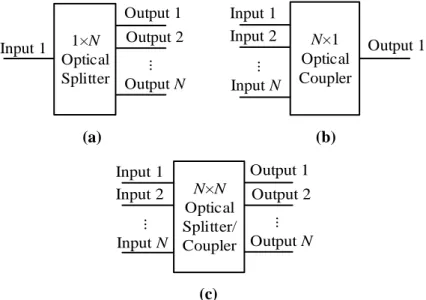

![Figure 4.2 - Four-node star network with a full-mesh logical topology [6].](https://thumb-eu.123doks.com/thumbv2/123dok_br/18906279.935875/60.892.165.730.113.464/figure-node-star-network-mesh-logical-topology.webp)