Diversity and Distributions. 2020;26:699–714. wileyonlinelibrary.com/journal/ddi
|
699 Received: 9 October 2019|
Revised: 17 January 2020|
Accepted: 4 February 2020DOI: 10.1111/ddi.13047
B I O D I V E R S I T Y R E S E A R C H
Combining geostatistical and biotic interaction modelling
to predict amphibian refuges under crayfish invasion across
dendritic stream networks
Mário Mota-Ferreira
1,2| Pedro Beja
1,2This is an open access article under the terms of the Creative Commons Attribution License, which permits use, distribution and reproduction in any medium, provided the original work is properly cited.
© 2020 The Authors. Diversity and Distributions published by John Wiley & Sons Ltd 1EDP Biodiversity Chair, CIBIO/InBio,
Centro de Investigação em Biodiversidade e Recursos Genéticos, Universidade do Porto, Vila do Conde, Portugal
2CIBIO/InBio, Centro de Investigação em Biodiversidade e Recursos Genéticos, Instituto Superior de Agronomia, Universidade de Lisboa, Lisboa, Portugal Correspondence
Mário Mota-Ferreira, EDP Biodiversity Chair, CIBIO/InBio, Centro de Investigação em Biodiversidade e Recursos Genéticos, Universidade do Porto, Campus de Vairão, Vila do Conde, Portugal.
Email: [email protected] Funding information
Fundação para a Ciência e a Tecnologia, Grant/Award Number: SFRH/
BD/95202/2013; EDP Biodiversity Chair Editor: Xuan Liu
Abstract
Aim: Biological invasions are pervasive in freshwater ecosystems, often causing na-tive species to contract into areas that remain largely free from invasive species im-pacts. Predicting the location of such ecological refuges is challenging, because they are shaped by the habitat requirements of native and invasive species, their biotic interactions, and the spatial and temporal invasion patterns. Here, we investigated the spatial distribution and environmental drivers of refuges from invasion in river systems, by considering biotic interactions in geostatistical models accounting for stream network topology. We focused on Mediterranean amphibians negatively im-pacted by the invasive crayfishes Procambarus clarkii and Pacifastacus leniusculus. Location: River Sabor, NE Portugal.
Methods: We surveyed amphibians at 168 200-m stream stretches in 2015. Geostatistical models were used to relate the probabilities of occurrence of each spe-cies to environmental and biotic variables, while controlling for linear (Euclidean) and hydrologic spatial dependencies. Biotic interactions were specified using crayfish prob-abilities of occurrence extracted from previously developed geostatistical models. Models were used to map the distribution of potential refuges for the most common amphibian species, under current conditions and future scenarios of crayfish expansion. Results: Geostatistical models were produced for eight out of 10 species detected, of which five species were associated with lower stream orders and only one spe-cies with higher stream orders. Six spespe-cies showed negative responses to one or both crayfish species, even after accounting for environmental effects and spatial de-pendencies. Most amphibian species were found to retain large expanses of potential habitat in stream headwaters, but current refuges will likely contract under plausible scenarios of crayfish expansion.
Main conclusions: Incorporating biotic interactions in geostatistical modelling provides a practical and relatively simple approach to predict present and future distributions of ref-uges from biological invasion in stream networks. Using this approach, our study shows that stream headwaters are key amphibian refuges under invasion by alien crayfish.
[Correction statement added on 05 May 2020 after first online publication: the article title has been corrected in this version.]
1 | INTRODUCTION
Biological invasions are pervasive in freshwater ecosystems, where they are major drivers of native species declines (Strayer, 2010; Walsh, Carpenter, & Vander Zanden, 2016). Addressing this threat is challeng-ing, because once fully established the control of invasive species is often nearly impossible, which limits the management options to pro-tect native species. In some circumstances, the impacts of biological invasions may be partly offset by the presence of ecological refuges, which are habitats where a species can retreat, persist in for up to a few decades, and eventually expand from under changing environ-mental conditions (Davis, Pavlova, Thompson, & Sunnucks, 2013). Such refuges correspond to freshwater habitats unsuitable for in-vasive species, or areas where their spread is prevented by physical barriers such as waterfalls or culverts (Kerby, Riley, Kats, & Wilson, 2005; Rahel, 2013). Refuges may thus allow the persistence of at least some remnant populations of native species (e.g. Chapman et al., 1996; Grabowski, Bacela, Konopacka, & Jazdzewski, 2009; Habit et al., 2010; Radinger, Alcaraz-Hernández, & García-Berthou, 2019), making it a priority to understand where, why and how refuges can contribute to species conservation under biological invasion.
Species distribution models (SDM) incorporating biotic inter-actions provide a simple framework to quantify how one or more species influence the distribution of others (e.g. Wisz et al., 2013), making them useful to predict the location and drivers of refuges from invasions. A straightforward approach is to take the distribu-tion patterns of invasive species together with abiotic variables to model the occurrence of native species, and then use the ensuing models to predict the distribution of refuges under current and fu-ture invasion scenarios (Araújo & Luoto, 2007; Wisz et al., 2013). One problem is that SDMs for geographical range prediction assume equilibrium between species distribution and the environment, which is unwarranted when modelling range contractions by na-tive species in face of biological invasion (Elith, Kearney, & Phillips, 2010; De Marco, Diniz, & Bini, 2008; Václavík et al., 2012). A native species may occur in areas that will latter become unsuitable due to the expansion of an invasive species, or it may eventually be able to coexist only temporarily with the invasive species due to time lags in negative impacts (Crooks, 2005). In either case, SDMs built using snapshots of species distributions may overestimate the extent of refuges, eventually misdirecting conservation efforts towards areas where native species persistence is unlikely.
Incorporating predictors describing spatial autocorrelations in invasive species occurrences to account for unmeasured dispersal and colonization processes may help mitigating, albeit not solving, problems associated with non-equilibrium conditions in SDMs (De Marco et al., 2008; Václavík et al., 2012; Filipe, Quaglietta, Ferreira,
Magalhães, & Beja, 2017). For alien species invading river ecosys-tems, SDMs can be improved using geostatistical models accounting for spatial dependencies in physical and ecological processes across stream networks (Filipe et al., 2017; Lois et al., 2015; Lois & Cowley 2017). These models are similar to conventional mixed models, with species occurrence modelled in relation to environmental variables using a logistic function, and spatial autocorrelation considered in the random errors (Peterson & Ver Hoef, 2010; Peterson et al., 2013; Ver Hoef & Peterson, 2010; Ver Hoef, Peterson, & Theobald, 2006). The latter are specified as a mixture of covariance functions rep-resenting the strength of influence between sites as a function of their (a) straight-line (Euclidean) distances calculated overland; (b) hydrologic distances (i.e. distances along the waterlines) represent-ing flow-connected relations (tail-up models); and (c) hydrologic dis-tances irrespective of flow connection (tail-down models) (Ver Hoef & Peterson, 2010). This approach can easily incorporate biotic inter-actions by including predictors describing the occurrence or abun-dance of potentially interacting species in the fixed component (Lois et al., 2015, Lois & Cowley 2017). Another possibility is to develop a geostatistical model for the invasive species itself, and then use the fitted response (i.e. the probability of occurrence) in the native species model. This should be useful for predicting the location of refuges, as it would consider not only the current distribution of the invasive species, but also suitable areas that will eventually be colo-nized during the expansion process.
This study investigates the location and environmental drivers of refuges in dendritic stream networks, combining biotic inter-actions and geostatistical modelling to predict their spatial dis-tribution under current and future scenarios of invasive species expansion. We focused on interactions between amphibians and the exotic crayfish Procambarus clarkii and Pacifastacus leniusculus in the Iberian Peninsula, where there are no native crayfish (Clavero, Nores, Kubersky-Piredda, & Centeno-Cuadros, 2016). These cray-fishes are among the most widespread and damaging aquatic invad-ers (Lodge et al., 2012; Twardochleb, Olden, & Larson, 2013), which have expanded widely in Iberia since the 1970s due to multiple in-troductions for commercial purposes and subsequent natural dis-persal (Bernardo, Costa, Bruxelas, & Teixeira, 2011; Clavero, 2016; Gutiérrez-Yurrita et al., 1999). Invasive crayfish predate on amphib-ian eggs and larvae (Axelsson, Brönmark, Sidenmark, & Nyström, 1997; Cruz & Rebelo, 2005; Cruz, Rebelo, & Crespo, 2006b; Gamradt & Kats, 1996), and seem to have strong negative impacts on native amphibian populations in Iberian waters (Cruz et al., 2006a; Cruz, Rebelo, et al., 2006b; Cruz, Segurado, Sousa, & Rebelo, 2008) and elsewhere (Ficetola et al., 2011). The main amphibian refuges are probably temporary ponds far from permanent waters (Beja & Alcazar, 2003; Cruz, Rebelo, et al., 2006b; Ferreira & Beja, 2013), K E Y W O R D S
Alien invasive species, biological invasions, ecological refuges, frog, geostatistics, newt, species distribution models, stream ecology, toad
where crayfish cannot persist (Cruz & Rebelo, 2007). Refuges may also exist in small and intermittent Mediterranean streams, which often hold rich amphibian communities (de Vries & Marco, 2017) and where crayfishes are usually absent (e.g. Cruz & Rebelo, 2007; Filipe et al., 2017; Gil-Sánchez & Alba-Tercedor, 2002). To inves-tigate amphibian refuges from crayfish invasion, we (a) made a detailed survey of amphibian occurrence in a Mediterranean water-shed; (b) developed geostatistical models relating the occurrence of each amphibian species to environmental variables, the probabil-ities of crayfish occurrence (Filipe et al., 2017) and spatial depen-dencies; and predicted the spatial distribution of refuges under (c) current and (d) future scenarios of crayfish expansion. Our study can help improve conservation strategies for amphibians negatively affected by crayfish invasions, and more generally, it provides a framework for identifying refuges from biological invasions in den-dritic stream networks.
2 | METHODS
2.1 | Study area
The study was conducted in the river Sabor watershed (NE Portugal; N41º090–42º000, W7º150–6º150; Figure S1). Human population is low (8.5–28.7 inhabitants/km2; https://www.porda ta.pt/Munic ipios) following a process of land abandonment since the 1970s (Azevedo, Moreira, Castro, & Loureiro, 2011). Land cover is dominated by ex-tensive agriculture and pastureland, forest plantations, and natural vegetation (Caetano, Marcelino, & C. Igreja e I. Girão, 2018; Hoelzer, 2003). A large proportion of the watershed is included in the Natura 2000 network (Costa, Monteiro-Henriques, Neto, Arsénio, & Aguiar, 2007). The watershed covers a wide range of elevations (100–1,500 m above sea level), total annual precipitation (443–1,163 mm) and mean annual temperature (6.9–15.6°C). The climate is Mediterranean, with precipitation concentrated in October–March and virtually none in June–August. Most small streams dry out or become reduced to a series of disconnected pools during the dry months, though the main watercourse and the largest tributaries are permanent (Ferreira, Filipe, Bardos, Magalhães, & Beja, 2016). Two large hydroelectric reservoirs were built and filled just before this study, but otherwise the river is largely free-flowing. Crayfish were first reported in the Sabor watershed in the 1990s, with P. clarkii probably introduced by local people, while P. leniusculus was introduced in 1994 by Spanish authorities (Bernardo et al., 2011). P. clarkii is far more widespread than P. leniusculus, but both species seem to still be spreading, pos-sibly through natural dispersal along the stream network (Anastácio et al., 2015; Bernardo et al., 2011).
2.2 | Study design
The study was designed to obtain a comprehensive snapshot of stream-dwelling amphibian distributions, considering both species
such as Iberian frog (Rana iberica) and Iberian green frog (Pelophylax perezi) that occupy streams during their entire life cycle, and species such as fire salamander (Salamandra salamandra) and midwife toads (Alytes obstetricans and A. cisternasii) that have both terrestrial and aquatic phases, occupying streams mostly during the breeding and larval development periods. To adequately cover all species, sur-veys encompassed the main environmental gradients represented in the watershed, and they were carried out monthly during one year to account for differences in activity peaks and breeding phe-nology across species (e.g. Díaz-Paniagua, 1992; Ferreira & Beja, 2013). Yet, because it was logistically unfeasible to sample a suf-ficiently large number of sites each month, the sampling effort was distributed over the year, with different sites sampled in different months. Considering these constraints, we initially selected >200 potential sampling sites, based on previous studies (Ferreira et al., 2016; Filipe et al., 2017; Quaglietta, Paupério, Martins, Alves, & Beja, 2018) and new field surveys. Sites were constrained to cover all Strahler stream orders and to be at >1 km from each other. All sites were in wadable stream reaches (water depth < 1.20) to fa-cilitate amphibian surveys. From the overall set of potential sam-pling sites, we selected each month a subset of 30 sites, following a stratified random procedure to guarantee that comparable envi-ronmental conditions were covered each month, and thus avoiding space × time interactions. To do this, we divided the Sabor water-shed into three sub-basins (Figure S1), and randomly selected each month two sites of each Strahler stream order represented in each sub-basin. A total of 168 sites were surveyed (Figure S1), with each site visited at most twice, except sites in higher orders that were visited more often because they were relatively scarce in the wa-tershed. The river network, sub-basins and stream orders were ob-tained from CCM 2.1 (Catchment Characterization and Modelling database; Vogt et al., 2007). A detailed workflow of the procedures used to analyse the data is provided in the Supplementary Methods in Supporting Information.
2.3 | Field sampling
Sampling was carried out monthly in 2015, except in May due to lo-gistic constraints. At each sampling site and date, a 200-m stream reach was thoroughly surveyed for amphibians, including both adults and larvae. The survey was conducted by two observers walking slowly along the banks or wading in shallow water along the stream. Observers used dip nets to collect aquatic larvae and adults, and they systematically searched the stream banks for ter-restrial adults, using torches where necessary to survey cavities and other shaded areas. All amphibians found were identified to species level in situ and released thereafter. In a few cases, small unidentified larvae were preserved and identified in the labora-tory. During surveys, crayfish were also recorded and identified to species, and all individuals collected were eliminated following guidelines established by the Portuguese biodiversity conserva-tion agency.
2.4 | Environmental and spatial variables
Sampling sites were characterized using variables potentially af-fecting the distribution of stream-dwelling amphibians that could be extracted from digital maps (e.g. Cruz & Rebelo, 2007; de Vries & Marco, 2017), making it possible to predict species distributions across the entire watershed in relation to potential expansions of crayfish ranges. Each site was characterized using four environ-mental variables (elevation [Alt], total annual precipitation [Prec], Strahler's stream order [SO] and the probability of water presence during the dry season [Water] and two variables describing the po-tential for biotic interactions between amphibians and either P. clarkii [Pclar] or P. leniusculus [Plen] (Cruz, Rebelo, et al., 2006b; de Vries & Marco, 2017). We also included a multiplicative interaction between elevation and Strahler's stream order (SOxAlt), which was used to distinguish between small streams in the lowlands and small streams in mountain areas. Initially, we also considered other climatic vari-ables, but they were discarded because of strong correlations with precipitation and/or elevation. Although features of the surrounding landscape are known to affect stream-dwelling amphibians (Ficetola et al., 2011; Riley et al., 2005), these were not considered because preliminary analysis showed very minor effects of land cover vari-ables in our study area, possibly due to the dominance of natural vegetation and low-intensity land uses that are generally suitable for amphibians. Furthermore, adding land cover variables often caused model instability and convergence problems, possibly due to redun-dancies with other environmental variables already included in the models.
All variables were computed in a Geographic Information System (GIS) using ArcGis (ESRI, 2016). Elevation was taken from a DEM built from 1:25,000 topographic maps as in Ferreira et al. (2016). Total an-nual precipitation was extracted from WordClim 2 with a 30’ (≈1 km) resolution (Fick & Hijmans, 2017). Strahler's stream order was used as a proxy for habitat size and heterogeneity (Ferreira et al., 2016; Hughes, Kaufmann, & Weber, 2011), and it was extracted from CCM 2.1, which is based on a 100-m resolution digital elevation model (DEM; Vogt et al., 2007). The probability of water presence in the dry period was used because many Mediterranean amphibian spe-cies are associated with temporary water bodies (Beja & Alcazar, 2003; Ferreira & Beja, 2013; de Vries & Marco, 2017), and it was extracted from a model developed in a previous study (Ferreira et al., 2016). Variables describing biotic interactions were specified consid-ering the probability of occurrence of either P. clarkii or P. leniusculus, extracted from a previous geostatistical modelling of crayfish dis-tribution in the Sabor watershed (Filipe et al., 2017). These models were built using electrofishing data collected on 167 sites in summer 2012, and they showed that crayfish distributions were mainly asso-ciated with stream order, elevation and spatial dependencies across the stream network (Filipe et al., 2017). The models had reasonable predictive accuracy, for both P. clarkii (AUC = 0.963) and P. leniusculus (AUC = 0.823). Probabilities derived from distribution models were used instead of the actual crayfish presences/absences recorded at sampling sites, in order to project the distribution of each species
across the entire watershed, as well as to build scenarios of future crayfish expansion. All variables were standardized to have a mean of zero and a standard deviation of one to improve the interpret-ability of model coefficients (Schielzeth, 2010), and we screened for outliers and influential points that might bias coefficient estimates.
Spatial data necessary to account for spatial autocorrelation (see below) were obtained in a GIS using the Sabor watershed stream network extracted from CCM2.1 (Vogt et al., 2007), and the layer of survey sites. Estimates included the Euclidean and hydrologic dis-tances (total and downstream hydrologic disdis-tances) between every pair of sampling sites (Peterson & Ver Hoef, 2010). To deal with con-fluences in tail-up models, we also estimated watershed areas to weight the relative influence of the branching upstream segments (e.g. Peterson & Ver Hoef 2010). Spatial estimates were made using the Spatial Tools for the Analysis of River Systems (STARS) toolbox version 2.0.0 (Peterson & Ver Hoef 2014) for ArcGIS 10.2 (ESRI, 2016).
2.5 | Distribution modelling
Distribution models (SDM) were developed considering for each species only the occurrence data from the sampling months encom-passing its aquatic phase, and thus the periods when the species is detectable during stream surveys (Table S1). For instance, we con-sidered data from all sampling months for R. iberica and P. perezi, because they are largely aquatic and strongly attached to stream habitats all year round, while we only considered data from April– November and October–April for A. obstetricans and S. Salamandra, respectively, corresponding to their aquatic phases. This approach aimed at avoiding false negatives caused by species not using poten-tially suitable stream habitats during the terrestrial phase.
For each species, we developed three logistic models relating its presence/absence to either (a) only environmental predictors, (b) only biotic predictors or (c) environmental + biotic predictors, and a (d) geostatistical distribution model (Peterson et al., 2013). The logis-tic models were used to evaluate how considering biologis-tic interactions affected species perceived responses to environmental variables, and as preliminary steps in geostatistical model building. The geo-statistical model for each species included a fixed component cor-responding to a logistic function linking its probability of occurrence to environmental and biotic predictors, and random components ac-counting for spatial dependencies in the stream network (Peterson & Ver Hoef, 2010; Peterson et al., 2013; Ver Hoef & Peterson, 2010; Ver Hoef et al., 2006). As random components, we considered the Euclidean model, assuming that spatial dependencies among sites can occur overland, and the tail-up and tail-down covariance mod-els, assuming that spatial dependencies can also occur along the hydrological network independently of flow and/or only between flow-connected sites, respectively (Peterson & Ver Hoef 2010).
To build the logistic models for each set of predictors and spe-cies, we considered all combinations of predictors of each set and retained for inference the best subset model minimizing AIC
(Murtaugh, 2009). Autocorrelation in model residuals was visual-ized using Torgegrams, depicting how semivariance in the residuals of the best logistic models between pairs of sampling sites changed in relation to their hydrologic distances (Peterson et al., 2013). In Torgegrams, increasing semivariance reflects declining spatial de-pendency between points. The fixed component of the geostatisti-cal model for each species was then built considering the predictors included in the best environmental + biotic logistic model. The structure of the random components was assessed using the resid-uals of the environmental + biotic model following Quaglietta et al. (2018), by testing all combinations of alternative functions available in the R package “SSN” (Ver Hoef, Peterson, Clifford, & Shah, 2014) for the Euclidean and the hydrologic autocovariance functions, and retaining the model structure minimizing AIC. We then combined the variables selected for the fixed component with the best spa-tial structure to build the final model for each species. In all logistic models and in the fixed component of the geostatistical model, we considered significance level for individual predictors at p < .10, to reduce the likelihood of type II errors and thus the probability of missing true-negative effects of crayfish invasion.
The crayfish models previously developed by Filipe et al. (2017) were validated with the presence/absence data from the 2015 survey, using the area under the receiver operating curve (AUC) (Allouche, Tsoar, & Kadmon, 2006). Discrimination ability of amphib-ian models was estimated using predictions obtained by the “leave-one-out” cross-validation method, considering the overall prediction success, the AUC, Cohen's kappa and the true skill statistics (TSS) (Allouche et al., 2006; Václavíık, Kupfer & Meentemeyer, 2012). Prediction success was estimated using prevalence as the threshold for predicted presences (Liu, Berry, Dawson, & Pearson, 2005). All analyses were carried out in R (R Core Team, 2017), using MuMIn (Barton, 2016), “SSN” (Ver Hoef et al., 2014) and “modEvA” (Barbosa et al., 2018) packages.
2.6 | Distribution mapping under current and
future scenarios
To map the predicted distribution of each amphibian species under current conditions, we projected the distribution models on the stream network of the entire Sabor watershed. First, we divided the stream network into segments of a maximum length of 1,000 m using ArcGIS desktop (ESRI, 2016), and we extracted the value of environmental variables from the centroid of each segment. We then predicted the probability of each species occurring in the seg-ment using universal kriging within the “SSN” package (Ver Hoef et al., 2014). We considered segments occupied if the predicted oc-cupancy probability was above the species prevalence threshold (Liu et al., 2005).
To simulate how crayfish expansion might affect amphibians, we changed the value of variables describing biotic interactions as-suming a twofold, threefold and fivefold increase in the relative risk (Rr) of each crayfish species occurring at each site, using as baseline
the predictions from the geostatistical models of Filipe et al. (2017). The relative risk was defined as the odds ratio of the probabilities of crayfish occurrence under future and current conditions, where odds are the ratio of the probability of occurrence and the probabil-ity of absence. The probabilprobabil-ity of occurrence at each site under each scenario of future crayfish expansion was then computed using the expression
where pi and p′
i are the probabilities of crayfish occurrence at present
and in the future at site i. We considered 16 different invasion sce-narios, assuming changes in the distribution of each crayfish species at a time, and both crayfish species simultaneously. These scenar-ios of crayfish expansion were built considering empirical observa-tions showing that both species are still expanding in the watershed (Bernardo et al., 2011), and assume that populations will expand from the areas currently occupied and will progressively colonize streams with habitat conditions most suitable for each species based on Filipe et al. (2017). Although this is a simplistic model, it can still provide ap-proximate indications on potential amphibian refuges under crayfish expansion.
Future distributions of each amphibian species were predicted using either the non-spatial environmental + biotic logistic model or the spatial geostatistical model, which reflect different assump-tions on range change processes (Record, Fitzpatrick, Finley, Veloz, & Ellison, 2013). The non-spatial model assumes that amphibian distributions will change along with changes in crayfish occurrence, irrespective of amphibian current distributions. However, spatial structure is still implicit in predictions, because probabilities of cray-fish occurrence across the dendritic stream network were them-selves predicted using geostatistical models (Filipe et al., 2017). In the geostatistical model, spatial random effects act to draw the projected distributions back towards the observed distribution used to calibrate the model (Record et al., 2013). Therefore, the current and future distributions will be similar, unless there are strong neg-ative effects of biotic interactions. Prediction of future distributions was only made for amphibian species showing significant negative effects of crayfish occurrence. We did not consider climate change effects due to uncertainties regarding how climate will change in our relatively small area and how crayfish and amphibians will re-spond to such changes, though this should be the subject of further research due to potential interactions between climate change and biological invasion (Hulme, 2017).
3 | RESULTS
We detected a total of 10 amphibian species, the most widespread (>20% of sites) of which were P. perezi (69%), S. salamandra (28%) and R. iberica (26%) (Table S1). The frogs Discoglossus galganoi and Hyla
p� i (1−p� i) pi (1−pi) = Rr⟨=⟩ p� i= Rr.pi 1 + pi�Rr − 1� , for Rr = � 2,3,5�
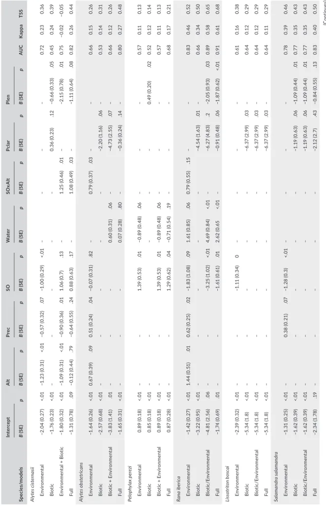
T A B LE 1 Pa ra m et er e st im at es a nd s um m ar y s ta tis tic s f or m od el s r el at in g t he p ro ba bi lit y o f o cc ur re nc e o f a m ph ib ia n s pe ci es t o v ar ia bl es de sc rib in g e nv iro nm en ta l e ff ec ts a nd b io tic i nt er ac tio ns i n t he S ab or w at er sh ed ( N E P or tu ga l) Sp ec ies /m od el s Inte rc ep t A lt Pr ec SO Wa te r SO xA lt Pc la r Pl en AU C K app a TSS B ( SE ) p B ( SE ) p B ( SE ) p B ( SE ) p B ( SE ) p B ( SE ) p B ( SE ) p B ( SE ) p Aly te s c is te rn as ii En vi ro nm en ta l −2 .0 4 ( 0. 27 ) <. 01 −1 .2 3 ( 0. 31 ) <. 01 −0 .5 7 ( 0. 32 ) .0 7 −1 .0 0 ( 0. 29 ) <. 01 – – – – 0. 72 0. 23 0. 36 B iot ic −1 .7 6 ( 0. 23 ) <. 01 – – – – – 0. 36 ( 0. 23 ) .1 2 −0. 66 (0. 33 ) .05 0. 45 0. 24 0. 39 En vi ro nm en ta l + B io tic −1 .8 0 ( 0. 32 ) <. 01 −1 .0 9 ( 0. 31 ) <. 01 −0 .9 0 ( 0. 36 ) .01 1. 06 ( 0. 7) .1 3 – 1. 25 ( 0. 46 ) .01 – −2 .1 5 ( 0. 78 ) .01 0. 75 −0.0 2 −0.0 5 Fu ll −1 .3 1 ( 0. 78 ) .0 9 −0 .1 2 ( 0. 44 ) .7 9 −0 .6 4 ( 0. 55 ) .24 0. 88 ( 0. 63 ) .17 – 1. 08 ( 0. 49 ) .0 3 – −1 .1 1 ( 0. 64 ) .0 8 0. 82 0. 26 0.4 4 Aly te s o bs te tr ic an s En vi ro nm en ta l −1 .6 4 ( 0. 26 ) <. 01 0. 67 ( 0. 39 ) .0 9 0. 51 ( 0. 24 ) .0 4 −0.0 7 (0. 31 ) .82 – 0. 79 ( 0. 37 ) .0 3 – – 0. 66 0.1 5 0. 26 B iot ic −2 .5 7 ( 0. 68 ) <. 01 – – – – – −2 .2 0 ( 1. 16 ) .0 6 – 0. 53 0. 14 0. 31 B io tic + E nv iro nm en ta l −3 .8 3 ( 1. 41 ) .01 – – – 0. 60 ( 0. 31 ) .0 6 – −4 .7 3 ( 2. 55 ) .0 7 – 0. 66 0.1 2 0. 26 Fu ll −1 .6 5 ( 0. 31 ) <. 01 – – – 0.0 7 (0. 28 ) .8 0 – −0 .3 6 ( 0. 24 ) .14 – 0. 80 0. 27 0.4 8 Pel op hy la x p er ez i En vi ro nm en ta l 0. 89 ( 0. 18 ) <. 01 – – 1. 39 ( 0. 53 ) .01 −0 .8 9 ( 0. 48 ) .0 6 – – – 0. 57 0. 11 0.1 3 B iot ic 0. 85 ( 0. 18 ) <. 01 – – – – – 0. 49 ( 0. 20 ) .02 0. 52 0.1 2 0. 14 B io tic + E nv iro nm en ta l 0. 89 ( 0. 18 ) <. 01 – – 1. 39 ( 0. 53 ) .01 −0 .8 9 ( 0. 48 ) .0 6 – – – 0. 57 0. 11 0.1 3 Fu ll 0. 87 ( 0. 28 ) <. 01 – – 1. 29 ( 0. 62 ) .0 4 −0 .7 1 ( 0. 54 ) .19 – – – 0. 68 0. 17 0. 21 Ra na ib eri ca En vi ro nm en ta l −1 .4 2 ( 0. 27 ) <. 01 1. 44 ( 0. 51 ) .01 0. 62 ( 0. 25 ) .02 −1 .8 3 ( 1. 08 ) .0 9 1. 61 ( 0. 85 ) .0 6 0. 79 ( 0. 55 ) .1 5 – – 0. 83 0.4 6 0. 52 B iot ic −3 .2 2 (0 .95 ) <. 01 – – – – – −4 .5 4 ( 1. 63 ) .01 – 0. 66 0. 34 0. 50 Bi ot ic/ En vi ronm en ta l −4 .8 1 ( 2. 56 ) .0 6 – – −3 .2 5 ( 1. 02 ) <. 01 4. 69 ( 0. 84 ) <. 01 – −6 .27 ( 4. 83 ) .2 −2 .0 5 ( 0. 93 ) .0 3 0. 89 0. 58 0. 65 Fu ll −1 .7 4 ( 0. 69 ) .01 – – −1 .61 (0 .61 ) .01 2. 62 ( 0. 65 <. 01 – −0 .9 1 ( 0. 48 ) .0 6 −1 .8 7 ( 0. 62 ) <. 01 0.9 1 0. 61 0. 68 Li sso tr ito n b osc ai En vi ro nm en ta l −2 .3 9 ( 0. 32 ) <. 01 – – −1 .1 1 ( 0. 34 ) 0 – – – – 0. 61 0.1 6 0. 38 B iot ic −5 .3 4 ( 1. 8) <. 01 – – – – – −6 .3 7 ( 2. 99 ) .0 3 – 0. 64 0.1 2 0. 29 Bi ot ic/ En vi ronm en ta l −5 .3 4 ( 1. 8) <. 01 – – – – – −6 .3 7 ( 2. 99 ) .0 3 – 0. 64 0.1 2 0. 29 Fu ll −5 .3 4 ( 1. 8) <. 01 – – – – – −6 .3 7 ( 2. 99 ) .0 3 – 0. 64 0. 11 0. 29 Sa lam and ra sa lam and ra En vi ro nm en ta l −1 .3 1 ( 0. 25 ) <. 01 – 0. 38 ( 0. 21 ) .0 7 −1 .2 8 ( 0. 3) <. 01 – – – – 0. 78 0. 39 0.4 6 B iot ic −1 .62 ( 0. 39 ) <. 01 – – – – – −1 .1 9 ( 0. 63 ) .0 6 −1 .0 9 ( 0. 44 ) .01 0. 77 0. 35 0.4 3 Bi ot ic/ En vi ronm en ta l −1 .62 ( 0. 39 ) <. 01 – – – – – −1 .1 9 ( 0. 63 ) .0 6 −1 .0 9 ( 0. 44 ) .01 0. 77 0. 35 0.4 3 Fu ll −2 .3 4 ( 1. 78 ) .19 – – – – – −2 .1 2 ( 2. 7) .4 3 −0 .8 4 ( 0. 55 ) .1 3 0. 83 0.4 0 0. 50 (Co nti nue s)
molleri were excluded from further analysis because they occurred at just one and two sites, respectively. P. clarkii and P. leniusculus were detected at 28% and 22% of sites surveyed for amphibians, with the models of Filipe et al. (2017) successfully predicting the presence/absence of each species (P. clarkii: AUC = 0.96; P. leniuscu-lus; AUC = 0.92; Figure S2).
Models including only environmental effects showed significant negative effects of stream order on the probability of occurrence of A. cisternasii, R. iberica, Lissotriton boscai, S. salamandra and Triturus marmoratus, and positive effects on P. perezi (Table 1). Altitude was negatively related to A. cisternasii, and positively so with A. obstetri-cans and R. iberica. Significant interactions between stream order and altitude were found for A. cisternasii and R. iberica, indicating in both cases that negative effects of stream order were weaker at higher elevations. Precipitation was negatively related to A. cisternasii, and positively so with A. obstetricans, R. iberica and S. salamandra. The probability of a stream segment retaining water in summer showed a negative relation with P. perezi and a positive relation with R. iberica. Models including only biotic interactions showed significantly nega-tive relations between P. clarkii and A. obstetricans, R. iberica, L. bos-cai, S. salamandra and T. marmoratus (Table 1). P. leniusculus was negatively related to A. cisternasii and S. salamandra, and positively to P. perezi. Bufo spinosus was the only species showing no significant environmental or biotic effects.
When combining environmental and biotic variables (Table 1), the effects of biotic interactions were retained for all species except P. perezi, while the type and significance of environmental effects often changed considerably. For L. boscai, S. salamandra and T. mar-moratus, only the negative effects of P. clarkii were retained in the best model. For R. iberica, the combined model highlighted a nega-tive effect of P. leniusculus and stream order, and a posinega-tive effect of the probability of water presence. For A. obstetricans, there was a negative effect of P. clarkii and a positive effect of water presence, while for A. cisternasii, there were negative effects of P. leniusculus and precipitation, and an interaction between stream order and elevation suggesting that the species was most likely to occur in higher stream orders at higher elevation, and the reverse at lower elevations.
Torgegrams suggested the occurrence of spatial dependencies in model residuals among flow-connected sites for R. iberica, L. bos-cai, S. salamandra and T. marmoratus, while spatial dependencies for flow-unconnected sites were apparent for S. salamandra and, partic-ularly, A. cisternasii (Figure S3). The tail-up component was included in the best covariance structure for A. obstetricans, R. iberica and S. salamandra, and the Euclidean component was included in the best models for A. cisternasii, P. perezi, L. boscai, S. salamandra and T. mar-moratus (Table 2). The tail-down component was only included in the best model for R. iberica. Overall, the spatial components accounted for a much larger amount of explained variation than the environ-mental + biotic effects (Table 2), and thus, the full models showed the best performance in terms of AUC, Cohen's Kappa and TSS (Table 1). The AUC of the full models was reasonable (0.80–0.91) for A. cisternasii, A. obstetricans, R. iberica and S. salamandra, but it was
Sp ec ies /m od el s Inte rc ep t A lt Pr ec SO Wa te r SO xA lt Pc la r Pl en AU C K app a TSS B ( SE ) p B ( SE ) p B ( SE ) p B ( SE ) p B ( SE ) p B ( SE ) p B ( SE ) p B ( SE ) p Tr itu ru s m ar m or at us En vi ro nm en ta l −1 .9 6 ( 0. 27 ) <. 01 – – −0 .9 2 ( 0. 29 ) <. 01 – – – – 0. 59 0. 14 0. 28 B iot ic −3 .4 2 ( 1. 10 ) <. 01 – – – – – −3 .6 5 (1 .9) .05 – 0. 59 0. 20 0.4 3 Bi ot ic/ En vi ronm en ta l −3 .4 2 ( 1. 10 ) <. 01 – – – – – −3 .6 5 (1 .9) .05 – 0. 59 0. 20 0.4 3 Fu ll −2 .6 0 ( 0. 85 ) <. 01 – – – – – −2 .2 2 ( 1. 31 ) .0 9 – 0. 66 0.0 4 0.0 8 N ote : F or e ac h s pe ci es , w e p ro vi de f ou r d iff er en t m od el s i nc or po ra tin g ( a) e nv iro nm en ta l v ar ia bl es ; ( b) b io tic i nt er ac tio ns ; ( c) e nv iro nm en ta l v ar ia bl es + b io tic i nt er ac tio ns ; a nd ( d) e nv iro nm en ta l va ria bl es + b io tic i nt er ac tio ns + s pa tia l d ep en de nc ie s a cr os s s tr ea m n et w or ks ( Fu ll) . V ar ia bl es i nc lu de d w er e e le va tio n ( A lt) , t ot al a nn ua l p re ci pi ta tio n ( Pr ec ), S tr ah le r's s tr ea m o rd er ( SO ), t he w at er pr es en ce p ro ba bi lit y ( W at er ) a nd t he p ro ba bi lit y o f t he p re se nc e o f e ith er Pr oc am bar us c lar ki i ( Pc la r) o r P ac ifas ta cus le ni us cu lus (P le n) . W e a ls o i nc lu de d a m ul tip lic at iv e i nt er ac tio n b et w ee n e le va tio n a nd st re am o rd er ( SO xA lt) . F or e ac h m od el , w e p ro vi de t he r eg re ss io n c oe ff ic ie nt e st im at es ( B) , t he ir s ta nd ar d e rr or s ( SE ) a nd p-va lu es , a nd t hr ee m ea su re s o f m od el p re di ct iv e a bi lit y: a re a u nd er t he r ec ei ve r op er at in g c ur ve ( A U C ), C oh en 's k ap pa a nd t ru e s ki ll s ta tis tic s ( TS S) . S pe ci es o bs er ve d p re va le nc e w as u se d a s t he t hr es ho ld t o c om pu te C oh en 's k ap pa , a nd t he t ru e s ki ll s ta tis tic s. T A B LE 1 (Co nti nue d)
low for the other species (0.64–0.68) (Table 1), which were thus not considered to map predicted distributions.
From a total of 1,468 km of waterlines in the Sabor watershed, the maps of predicted distributions based on the geostatistical models combining environmental, biotic and spatial predictors indicated that the species with most potential habitat was S. sal-amandra (64.6% of total stream length), followed by A. obstetri-cans (51.0%), A. cisternasii (48.4%) and R. iberica (38.9%) (Figure 1). S. salamandra occurred in lower order streams throughout the basin, while both Alytes species were widespread in lower and middle order streams, with A. cisternasii occurring primarily in the south and southeast and A. obstetricans in the north and north-west (Figure 1). R. iberica was largely restricted to lower order streams in more mountainous areas of the north and northwest. The distributions of these species correspond to streams with low probability of occurrence of both invasive crayfish, but that were predicted to be progressively colonized under the invasion scenar-ios (Figures S4 and S5). Expansion of crayfish through the stream network was predicted to decrease the length of potential stream habitat for amphibians, with each species becoming progressively more confined to first- and second-order streams (Figure 2, Table S2). Predictions using spatial models suggested that the length of habitat of A. cisternasii will decline up to about 30% due to the expansion of P. leniusculus, while a reduction of about 7% was pre-dicted for A. obstetricans due to the expansion of P. clarkii. The potential habitat for R. iberica and S. salamandra was expected to decline by about 20%, due to the joint expansion of P. leniusculus and P. clarkii. Non-spatial models predicted even larger declines for A. cisternasii (up to 69.9%), A. obstetricans (51.3%) and R. iberica (53.9%), but not as much for S. salamandra (24.1%) (Figure 2, Table S2). For the latter species, there were upstream areas in the far north that were predicted to be occupied by the non-spatial model but not by the spatial model (Figure 2), suggesting that
environmentally suitable habitats may remain unoccupied due to spatial processes.
4 | DISCUSSION
Our study showed the value of combining geostatistical and bi-otic interaction modelling to quantify the spatial consequences of biological invasions on native species in dendritic stream net-works, and to predict the spatial distribution of ecological refuges under current and future invasion scenarios. Using this approach, we confirmed the strongly negative interactions between invasive crayfish and amphibians (Cruz, Pascoal, et al., 2006a; Cruz, Rebelo, et al., 2006b; Ficetola et al., 2011; Riley et al., 2005), while ad-vancing previous knowledge by showing that such interactions are causing marked range contractions at the watershed scale in many species, and that this effect may intensify in the future under plau-sible scenarios of crayfish expansion. Moreover, our results show that stream headwaters (i.e. stream orders 1 and 2; Finn, Bonada, Múrria, & Hughes, 2011) represent key refuges from crayfish in-vasion for many amphibian species, as these streams dry out for more or less extended periods during the dry season (Ferreira et al., 2016) and are thus expected to remain largely free from crayfish impacts (Cruz & Rebelo, 2007; Filipe et al., 2017). Overall, our study reinforces the conservation importance of stream headwaters in the Mediterranean region, which are increasingly perceived to play key roles as refuges from biological invasions and other human-me-diated disturbances, both for amphibians (de Vries & Marco, 2017) and other vulnerable species (Quaglietta et al., 2018; Sousa et al., 2019). Our approach may be applied to other aquatic species, with major implications for conservation and management by permitting a better identification of areas acting as ecological refuges under biological invasion.
TA B L E 2 Covariance structure selected for the geostatistical models of each species, indicating the percentage of variation accounted
by the fixed and each spatial component of the final models. For each spatial component, we indicate the function used to specify the covariance structure
Species Environment + Biotic
Spatial
Nugget
Tail Up Tail Down Euclidean
Alytes cisternasii 3.7 – – 32.2 (Gaussian) 64.1
Alytes obstetricans 1.6 98.4 (Epanech) – – ≈0.0
Pelophylax perezi 4.4 – – 31.0 (Cauchy) 64.6
Rana iberica 9.9 27.5 (Mariah) 30.0 (Spherical) – 32.6
Lissotriton boscai 2.8 – – ≈0.0 (Spherical) 97.2
Salamandra salamandra 3.9 17.7 (Spherical) – 0.28 (Gaussian) 50.9
Triturus marmoratus 1.9 – – 0.22 (Gaussian) 76.6
F I G U R E 1 Maps showing the observed presences/absences of four amphibian species in the river Sabor watershed (NE Portugal) in
2015, and their potential distributions predicted from geostatistical models combining environmental effects, biotic interactions and spatial dependencies across the dendritic stream network. The threshold for predicted presences was set equal to the observed prevalence of each species
(c) Rana i b e r i c a (d) Salamandra s a l a m andra (a) Alytes c i s t e r n a si i 0 5 10km Legend Observations ( Absences ( Presences Preditions Unsuitable habitat Suitable habitat Reservoir Inundated Area (b) Alytes o b s t e t r i c a n s
4.1 | Study limitations
Although our study had some limitations, it is unlikely that they af-fected our main conclusions in any significant way. One potential problem is that we sampled streams from first to sixth orders, and it may be argued that the prevalence of amphibian species may be un-derestimated in larger streams due to lower detectability. Although this can be addressed by modelling occupancy while controlling for detectability (e.g. MacKenzie et al., 2017), this was not possible in our case because occupancy-detection models accounting for hy-drological tail-up and tail-down spatial dependencies have yet to be developed. To deal with this problem, we have surveyed only wad-able streams and increased the sampling effort in larger streams, which should have contributed to achieve comparable detectability across stream orders. This is supported by the higher prevalence
of P. perezi and the crayfish P. clarkii in higher than lower orders, which suggest that we did not miss species known to occur in larger streams (Cruz, Rebelo, et al., 2006b; Filipe et al., 2017). Moreover, species distribution patterns observed in our study were consist-ent with those of others focusing on stream-dwelling amphibians in Iberia (Cruz, Rebelo, et al., 2006b; de Vries & Marco, 2017), thereby suggesting that they were not artefacts shaped by sampling biases. Another potential problem is that amphibian models were based on large-scale variables, while ignoring local drivers such as the struc-ture and composition of riparian vegetation, the land uses surround-ing streams and water quality (Crawford & Semlitsch, 2007; Guzy, Halloran, Homyack, & Willson, 2019; Riley et al., 2005). Missing these variables might have reduced the predictive ability of our mod-els, but we believe that the variables considered are relevant to in-vestigate large-scale distribution patterns, as observed for instance
F I G U R E 2 Maps of potential
distributions of four amphibian species under the worst case scenario of future crayfish expansion in the river Sabor watershed (NE Portugal). The scenario was built considering a fivefold increase in the relative risk of crayfish occurrence (both P. clarkii and P. leniusculus) at each stream segment in relation to the baseline scenario corresponding to the predicted distribution of each species in 2012 (Filipe et al., 2017). In each map, we indicate the waterlines where potential habitat will remain available (suitable habitat), and those where potential habitat will be lost (lost habitat) in relation to the baseline scenario. Maps were produced using predictions from either spatial or non-spatial (i.e. including only environmental effects and biotic interactions) models [Correction statement added on 05 May 2020 after first online publication: Figure 2 was previously merged and has been divided into two parts in this version.]
(c) Spatial
predictions (d)predictions Non-spatial
0 5 1 0km Legend Predictions Unsuitable habitat Lost habitat Suitable habitat
Alytes obstetricans
(a) Spatial predictions (b) Non-spatial predictionsAlytes cisternasii
in other species modelled in the Sabor watershed (Ferreira et al., 2016; Filipe et al., 2017; Quaglietta et al., 2018). Nevertheless, while our models should be informative to understand broad changes in amphibian distributions in relation to crayfish invasion, they may be less useful to predict whether a given species will be present at any given site, which may be strongly affected by more local environ-mental conditions.
4.2 | Effects of biotic interaction and environmental
effects on amphibian distributions
The negative responses of amphibians to invasive crayfish ob-served in the Sabor watershed were comparable to those reported elsewhere (Cruz, Pascoal, et al., 2006a; Gamradt & Kats, 1996;
Gamradt, Kats, & Anzalone, 1997; Girdner et al., 2018; Nyström, Birkedal, Dahlberg, & Brönmark, 2002; Nyström, Svensson, Lardner, Brönmark, & Granéli, 2001). However, impacts of P. leni-usculus are reported here for the first time in Iberia, though this crayfish was already associated with local amphibian declines in Sweden (Nyström et al., 2002, 2001). We also confirmed that crayfish impacts seem to be particularly strong on urodela (sala-mander and newts), possibly because their eggs and larvae are highly vulnerable to introduced predators (Cruz, Rebelo, et al., 2006b; Gamradt & Kats, 1996; Gamradt e al. 1997; Girdner et al., 2018). Mediterranean amphibians may be especially vulnerable to crayfish because many species are adapted to live in water bodies that dry out in summer and are naturally free from fish and other large predators (e.g. Beja & Alcazar, 2003; Ferreira & Beja, 2013), and thus may be less adapted to cope with crayfish
(g) Spatial
predictions (h)predictions Non-spatial
Salamandra salamandra
(e) Spatial
predictions (f)predictions Non-spatial
Rana iberica
0 5 1 0km Legend Predictions Unsuitable habitat Lost habitat Suitable habitat F I G U R E 2 (Continued)predation than species living in permanent waters (Cruz, Rebelo, et al., 2006b; Nunes et al., 2011). This is supported by the lack of negative effects on P. perezi, which is known to thrive in perma-nent waters where predators are abundant (Beja & Alcazar, 2003; Cruz, Rebelo, et al., 2006b; Ferreira & Beja, 2013). We also found no negative effects on B. spinosus, which is widespread in perma-nent waters and seems to be less vulnerable to predators due to its toxic eggs and larvae (Cruz & Rebelo, 2005), though a previous study reported negative impacts of P. clarkii (Cruz, Rebelo, et al., 2006b). In contrast, we found negative impacts on A. cisternasii, which is associated with more permanent water bodies and was found previously to be unaffected by crayfish (Cruz, Rebelo, et al., 2006b). However, that study was carried out in an area where only P. clarkii occurred, while in our study, we only found significant negative effects for P. leniusculus, suggesting that impacts may differ among crayfish species. P. leniusculus also showed strong negative effects on R. iberica, possibly because this species occurs primarily in mountainous streams largely unsuitable for P. clarkii (Filipe et al., 2017). These results suggest that invasion by multiple crayfish species may be more serious than invasion by a single species, by increasing the types of habitats invaded (Filipe et al., 2017) and the number of species vulnerable to predation.
Although our study showed that many amphibian species were associated with stream headwaters, different species occurred in different areas, probably due to differences in ecological require-ments. For instance, environmental models suggested that while both A. cisternasii and A. obstetricans were mainly found in lower and middle stream orders, the former favoured areas with lower precipitation at low elevation, while the reverse was found for the latter. This probably explains their largely parapatric distributions in the study area, as observed at broader spatial scales (Reino et al., 2017). Models for R. iberica also confirmed their preference for small permanently flowing streams in mountainous areas (Bosch, Rincón, Boyero, & Martínez-Solano, 2006; Rodríguez-Prieto & Fernández-Juricic, 2005). Many of these environmental effects, however, were lost from the best models or became non-significant, once biotic in-teractions were included. In some cases, there were also changes in the significant environmental effects, with for instance the selec-tion of permanently flowing waters by A. obstetricans only becoming apparent after controlling for the effects of P. clarkii. These results support the idea that the two exotic crayfish are key drivers con-straining amphibian distributions in our study area, limiting the range of environmental conditions where they can be found.
4.3 | The role of spatial dependencies across the
stream network
Incorporating spatial covariance structure greatly enhanced the dis-tribution models, with both Euclidean and hydrologic distances often included in the best models. The Euclidean component was important for A. cisternasii, P. perezi, S. salamandra and T. marmoratus, suggest-ing that adjacent streams have more similar occupancy status than
streams farther apart, which may be due to the dispersal of individuals overland (e.g. Semlitsch, 2008) or similarities regarding unmeasured spatially structured environmental variables (e.g. land cover/land uses). Euclidean effects may be particularly important in species associated with headwaters, because nearby streams may be flow-unconnected and at long hydrologic distances from each other. The tail-up compo-nent was important for A. obstetricans, R. iberica and S. salamandra, which may be a consequence of flow-connected sites having similar environmental conditions, but also of similarities in occupancy status due for instance to downstream drift of larvae or their active swim-ming upstream. The tail-down component was only important for R. iberica, possibly reflecting dispersal movements along the waterlines irrespective of flow, as this is a species strongly attached to riverine habitats during the adult and larval stages, and may have low dispersal ability overland as suggested by the lack of the Euclidean component.
In the full mixed models, spatial dependencies accounted for a far greater proportion of variation in species occurrences than the fixed component, as observed in other studies using geostatisti-cal tools (Filipe et al., 2017; Lois et al., 2015, Lois & Cowley 2017; Quaglietta et al., 2018). This was probably because the fixed com-ponent was specified using variables that are spatially structured, either Euclidean (e.g. precipitation, elevation) or hydrologic (e.g. stream order), and thus, their effects were reduced after considering spatial dependencies. It is worth noting, however, that variables de-scribing biotic interactions generally remained significant in the full models, further emphasizing their importance. The fixed component would probably have had a larger share of the explained variation, probably contributing to the overall predictive power of the models, if we had considered variables describing more local environmental conditions that are known to affect stream-dwelling amphibians (e.g. Crawford & Semlitsch, 2007; Guzy et al., 2019; Riley et al., 2005). Future studies combining drivers operating at landscape and local scales should thus be developed, which would likely improve predic-tions on potentially favourable areas across the watershed.
4.4 | Predicting amphibian refuges under
crayfish invasion
Despite the limited explanatory power of the spatial distribution mod-els, the mapping of predicted distributions clearly showed that further crayfish expansions will likely result in amphibian range contractions, with populations becoming progressively more encroached in lower order streams. This could be inferred quantitatively for four species with geostatistical models with sufficient predictive ability (A. cis-ternasii, A. obstetricans, R. perezi and S. salamandra), but will probably occur also for the other two species showing negative associations with crayfish occurrence (L. boscai and T. marmoratus) in ours and other studies (Cruz, Rebelo, et al., 2006b). The non-spatial models (i.e. including only environment + biotic interactions) predicted even stronger declines in the availability of potential habitats, particularly for A. cisternasii, A. obstetricans and R. iberica. This is because spatial models anchor model predictions to the current distribution of each
species, and thus may be regarded as conservative because they add inertia against abrupt changes in distribution driven by environmental factors (Record et al., 2013). In contrast, the non-spatial models are only driven by changes in crayfish occurrence irrespective of the spa-tial structure in current amphibian distribution, thereby disregarding possible spatially structured population processes shaping amphib-ian species distributions (Record et al., 2013). Therefore, we expect that the extent of range contractions will be somewhere in-between the predictions of spatial and non-spatial models, which may thus be substantial for A. cisternasii (up to 30.6%–69.6%), A. obstetricans (6.8%-51.3%) and R. iberica (20.6%-53.9%), though only moderate to S. salamandra (22.3%–24.1%). The consequences of such changes for population persistence should be evaluated in future studies, as it is likely that the risk of local extinctions will be high for small and isolated populations confined to headwater streams.
4.5 | Conservation and management implications
Invasion by alien crayfish is a major cause of concern for amphibian conservation (e.g. Cruz, Pascoal, et al., 2006a; Gamradt & Kats, 1996; Gamradt et al., 1997; Girdner et al., 2018; Nyström et al., 2001, 2002). Addressing this problem is challenging, because once established in-vasive crayfish populations are virtually impossible to eradicate, and thus, remediation of ecosystems invaded by crayfish has met very limited success (Gherardi, Aquiloni, Diéguez-Uribeondo, & Tricarico, 2011; Stebbing, Longshaw, & Scott, 2014). Furthermore, many inva-sive crayfish species are still expanding within and across watersheds (e.g. Bernardo et al., 2011; Kouba, Petrusek, & Kozák, 2014), and so the problem is likely to get worse in the future. In this context, our study suggests that stream headwaters may be critical for the per-sistence of many stream-dwelling amphibian species, at least in the Mediterranean region, as they often hold diverse amphibian commu-nities (de Vries & Marco, 2017) and are likely to provide refuges with minimal or no crayfish impacts (Filipe et al., 2017). These headwaters correspond not only to small order streams in mountainous areas, as those inhabited for instance by A. obstetricans and R. perezi, but also to small temporary streams at lower elevation, which seem to be pre-ferred by species such as A. cisternasii. Overall, therefore, headwater streams should be regarded as priority targets for conservation, requir-ing the preservation of habitat conditions compatible with amphibian persistence. Although the ecological requirements of stream-dwelling amphibians are poorly known in the Iberian Peninsula (de Vries & Marco, 2017), it is likely that conservation efforts should target pre-serving water quality, natural flow regimes, well-developed riparian vegetation and suitable terrestrial habitats (e.g. Crawford & Semlitsch, 2007; Guzy et al., 2019; Riley et al., 2005). Furthermore, efforts should be made to avoid the colonization of headwater refuges by invasive crayfish such as P. leniusculus, which is fast expanding into new areas (Anastácio et al., 2019; Bernardo et al., 2011), and may be able to colo-nize mountainous headwater streams inhabited by endemic amphib-ians such as R. iberica (Filipe et al., 2017). This would require monitoring crayfish populations in key amphibian refuges, which should be used totrigger careful management programmes if the risk of negative impacts become unacceptably high, involving for instance the implementation of control or eradication programs, and/or the introduction of physi-cal barriers to crayfish dispersal (Gherardi et al., 2011; Sousa et al., 2019; Stebbing et al., 2014). Although such conservation measures may require considerable efforts and may only be applicable in some areas, maintaining stream headwaters free of invasive crayfish should have major conservation benefits for a range of endangered species (Quaglietta et al., 2018; Sousa et al., 2019; de Vries & Marco, 2017) and for aquatic biodiversity in general (Finn et al., 2011; Meyer et al., 2007).
5 | CONCLUSIONS
Under biological invasion, many native species are becoming con-fined to refuges where invasive species are still absent or scarce, and thus may hold remnant populations of high conservation value (e.g. Chapman et al., 1996; Grabowski et al., 2009; Habit et al., 2010; Radinger et al., 2019). This study provides a framework to predict the location and environmental drivers of such refuges, using geostatis-tical tools to model native species responses to exotic species while controlling for environmental effects and spatial dependencies across dendritic stream networks (Filipe et al., 2017; Peterson et al., 2013). This approach is relatively simple and can be used where only snapshot surveys on the occurrence patterns of native and invasive species are available, though it can be easily extended to deal with data on distri-butional dynamics (Quaglietta et al., 2018) and additional complexities such as climate change (Peterson et al., 2013). This framework may be generally useful to understand the distributional consequences of in-teractions between native and invasive species, providing information on the location of potential refuges where conservation efforts should concentrate, and on management actions required to enhance the per-sistence of remnant populations within refuges.
ACKNOWLEDGEMENTS
This work was carried out in the scope of the Baixo Sabor Long Term Ecological Research Site. Funding was provided by EDP and by the Portuguese Science and Technology Foundation (FCT). MMF was supported by the FCT PhD grant SFRH/BD/95202/2013, and PB by EDP Biodiversity Chair. We thank collaboration in fieldwork by Ninda Batista, Joana Pinto, Erika Almeida and Ivo Rosa.
DATA AVAIL ABILIT Y STATEMENT
The SSN files including information on species presence/absence and on the spatial topology of the stream network and sampling sites are provided in Dryad (https://doi.org/10.5061/dryad.mw6m9 05tb), together with the R scripts and additional files needed to repeat all analysis using the SSN package. The raw data on amphibian occur-rences are available from the authors upon request.
ORCID
Mário Mota-Ferreira https://orcid.org/0000-0002-0595-620X Pedro Beja https://orcid.org/0000-0001-8164-0760