Adaptive Time Synchronization Protocol for BANS

(1)

Paulo Fernando Pereira Vilares

Adaptive Time Synchronization

Protocol for BANs

Departamento de Ciˆ

encia de Computadores

Faculdade de Ciˆ

encias da Universidade do Porto

(2)

Adaptive Time Synchronization

Protocol for BANs

Disserta¸cão submetida à Faculdade de Ciências da

Universidade do Porto como parte dos requisitos para a obten¸c˜ao do grau de Mestre em Engenharia de Redes em Sistemas Inform´aticos

Orientador: Pedro Brand˜ao

Departamento de Ciˆencia de Computadores Faculdade de Ciˆencias da Universidade do Porto

(3)

To my beloved ones

(4)

I gratefully acknowledge the guidance and assistance of my supervisor Prof. Pedro Brand˜ao, his valuables ideas and suggestions were priceless. I am also very grateful for giving me this great opportunity of learning.

(5)

Abstract

The constant miniaturization of electronic devices has enabled new types of networks. The development of tiny low-power devices capable of performing sensing enabled wire-less architectures that monitor different types of areas (industrial, natural habitats, etc.) with different objectives and constraints. If we add actuators to the ensemble, and restrict the network to the human body, we have Body Area Network (BAN) architectures. BANs can assume different purposes and enable new applications in the areas of sport monitoring, personal entertainment and emergency response solutions for better healthcare.

The variety of purposes and applications that a BAN can cover, translates into a heterogeneity of requirements (network use, hardware, energy consumption, etc.), that depend on the application’s objectives. These applications, in addition to monitoring and data collection, need to correlate data from different sensor nodes. For this cor-relation to be useful and correctly related, time synchronization between the different nodes is of essence.

We propose a time synchronization protocol specific for BANs that addresses the heterogeneity of sensors and applications using the network. We argue that existing work does not tackle and use these characteristics. Most of these time synchronization protocols are designed to accomplish the best accuracy possible, disregarding the application needs. This leads to an inefficient use of nodes’ resources. Our objective is to be accurate, but accurate according to the application requirements. This allows the node to save energy by being able to sleep more often

(6)

(7)

List of Tables

2.1 Application requirements (input from [18, 15]). . . 28 2.2 Characteristic between WSN and BAN (input from [18]). . . 34 5.1 Node simulation parameters. . . 58 5.2 Simulation parameters for the ECG and Temperature sensor node. . . . 66 5.3 Data and synchronization messages produced by node 1 (ECG) and

node 2 (Temperature). . . 66

(12)

(13)

List of Figures

1.1 Main characteristics of a WBAN compared with WSN (Reference

val-ues). Based on [18]. . . 18

2.1 Sources of time delays inherent to communication [20]. . . 25

2.2 Actuators and sensors in a BAN [4]. . . 28

2.3 LTS scheme for pair-wise synchronization [29]. . . 31

2.4 RBS critical path analysis for traditional time synchronization protocols (left) and RBS (right) [9]. . . 33

3.1 Message exchange for the synchronization phase. . . 38

3.2 Node clock adjustment flowchart. . . 40

3.3 Time synchronization timestamp. Frame format based on the IEEE 802.15.6 [14]. . . 41

3.4 Spare time for synchronization request. . . 42

3.5 Slave node resynchronization state machine. . . 43

4.1 Castalia module structure from [23]. . . 48

4.2 Node composite module from [23]. . . 49

4.3 Inheritance diagram for TimerService class. . . 50

4.4 Call graph for the getClock() method. . . 51

4.5 Call graph for the update drift function. . . 53

4.6 Inheritance diagram for the NewSyncProtocol class. . . 53 13

(14)

4.8 Modules interaction for a received synchronization message. . . 55 4.9 Modules interaction for a transmitted (from base station)

synchroniza-tion message. . . 56 5.1 Clock drift scenarios. Simulation runs for 3600 seconds (note that the

y-axis scale is different for the c)). . . 59 5.2 Node error with and without the sleep functionality. The error bars

represent a 95% confidence interval. . . 60 5.3 Node error without drift compensation. The error bars represent a 95%

confidence interval. . . 61 5.4 Consumed energy and number of sync messages, with/without sleep. . 62 5.5 Number of synchronization messages, with/without drift compensation. 63 5.6 Energy consumed and node error. Normal conditions scenario.

Syn-chronization interval is 5 seconds. The error bars represent a 95% confidence interval. . . 64 5.7 Energy consumed and node error for a drastic scenario. Synchronization

interval is 30 seconds. The error bars represent a 95% confidence interval. 65

(15)

Chapter 1 Introduction

Our work lies in two main areas: Body Area Networks (BAN) and Time Synchroniza-tion. More specifically we define a time synchronization protocol specific for BANs. In this introduction we describe the context of our work and the constraints of time synchronization in Body Area Networks. Our contribution is presented at the end.

1.1 Body Area Networks

The constant miniaturization of electronic devices has enabled the development of tiny low-power devices capable of performing sensing, computing and communication tasks [21]. These systems have enabled wireless sensor network (WSN) architectures that monitor different types of areas (industrial, natural habitats, etc.) with different objectives and constraints. Body Sensor Networks share some similarities with WSN but add different constraints: more heterogeneous sensors in the network, different applications and especially a different usage of the network itself [18]. By adding actuators to the ensemble, we have Body Area Network (BAN) architectures.

We can define a Body Area Network as a network of small devices (placed in or around the body), able to measure and collect data for monitoring a person (sensor node) and in some cases take a specific action (actuator). The nodes (sensor and actuator) communicate with each other and with a central node. The central node acts as a coordinator of the network and is a more powerful node (processing, storage, energy, etc.). To remove any ambiguity that may occur, from now on we will refer to the central node as Base Station (BS), and the sensors and actuators as only nodes. The

(16)

nodes can measure physiologic data (body temperature, electrocardiogram (ECG), oximetry, etc.), position, acceleration, etc. and in some cases react (pacemaker). This network can assume different purposes and enable new applications in the areas of sport monitoring, personal entertainment, emergency response and can provide effective solutions for better healthcare and personal wellbeing [18, 21]. The IEEE 802.15 task group 61_{, is a task group dedicated to BANs that defines ”a standard}

for short-range, wireless communication in the vicinity of, or inside, a human body (but not limited to humans). It uses existing industrial scientific medical (ISM) bands as well as frequency bands approved by national medical and/or regulatory authorities.”[14]. The group suggests a variety of applications divided in medical and non-medical (including entertainment) applications, some examples are [19]: Medical applications:

• Monitoring physiological parameters (Electroencephalogram EEG, Electrocar-diogram ECG, temperature, blood pressure, glucose and heart rate);

• Disability assistance (fall detection, muscle tension monitor and stimulation); • Sport training and performance (fatigue and battle readings);

• Remote control of medical devices (insulin pump, pacemaker and hearing aid). Non-medical applications:

• Entertainment applications (gaming and social networking); • Data file transfer (digital camera, scanner and digital player);

• Real-time video and audio streaming (music for headsets, voice and video com-munication).

With the last examples in mind, the motivation for our work rises from the variety of purposes and applications that a BAN can cover. This translates into a heterogeneity of requirements (network use, hardware, energy consumption, etc.), that depend on the application’s objectives (which is a key point in our work). These applications, in addition to monitoring and data collection, need to correlate data collected from different nodes [21], and properly time the occurrence of physical events. For this cor-relation to be useful and correctly related, time synchronization between the different nodes is of essence.

(17)

CHAPTER 1. INTRODUCTION 17

1.2 Time Synchronization

Time synchronization in distributed systems aims to provide a minimum drift between the different clocks of the system nodes. As clocks pulse this pulse frequency will tend to differ between different clocks, i.e., clocks will drift. The drift can occur due to oscillator’s instability, temperature and battery voltage variations [24, 10]. Another relevant characteristic of the clock is when the pulse occurs. Different clocks will pulse at different times, leading to skew. Time synchronization tries to minimize both errors.

Distributed systems will rely on message exchange to assess the differences and use them to correct the internal clocks. However, inherent to communications are delays. As described in [20] these times are send, access, transmission, propagation, reception and receive time. Send and receive time are concerned with message ”building” and accessing the MAC stack from the operating system’s perspective. Access time is related to access to the communication medium and is highly non-deterministic as it depends on medium usage. Transmission and reception time are related to the radio capabilities and throughput. Propagation time is related to the actual physical transmission on the medium, which in wireless networks is usually the air using radio-frequency. Given the short distances of WSNs and BANs this time is usually less than a µs.

In wireless networks time synchronization has several uses. Time synchronization plays a key service for different purposes, where some examples are: time of occurrence of physical events, localization and to share the communication medium in time division access models. The most notably is the correlation of timed events. TDMA (Time Division Multiple Access) based MAC protocols, need it to correctly time share the transmission medium and thus avoid collisions and optimize energy usage [25]. The time of occurrence of physical events is crucial to correlate data from different sources. The variety of uses (applications) and the different constraints from traditional networks (limited resources and network use), make time synchronization more difficult to achieve. Which leads us to the next section.

1.3 Time Synchronization in Body Area Networks

As we state in section 1.1, the applicability of BANs covers several areas, and can have a variety of applications. This translates to a diversity of hardware on which

(18)

sensors will be deployed and different time accuracy demands from the applications. These requirements influence the power consumption needed by each node to maintain synchronized clocks. Several time synchronization protocols have been proposed. Traditional time synchronization protocols, such the Network Time Protocol (NTP) [22], are used in large scale in distributed systems. However, these protocols are inappropriate for BANs due to their complexity and high resource requirements. BAN nodes have limited resources (energy, processing, memory, etc.).

Time synchronization protocols proposed for networks that have similarities with BANs, namely protocols for WSNs have also been proposed. WSNs have some similarities with BANs, but with different constraints. Figure 1.1 further illustrates the differences between WSNs and Wireless BANs (WBANs). In the figure values are indicative. WBANs cover the full spectrum of the characteristics.

Figure 1.1: Main characteristics of a WBAN compared with WSN (Reference values). Based on [18].

From figure 1.1 we can see the following main characteristics /challenges:

• BANs will have different types of sensors (heterogeneous nodes) in the network (Electrocardiogram (ECG), temperature, acceleration, oximetry, position, etc.); • They will also have different applications using the network (post-operative heart

(19)

CHAPTER 1. INTRODUCTION 19 • BANs have to support a high density of heterogeneous nodes (placed in or around

the body) with acceptance for the user, i.e. simple and non invasive nodes; • BAN node needs to be used without interruption (specially implanted nodes)

and power supply can be difficult or inaccessible. Energy efficiency is essential to improve the node’s lifetime;

• The cost structure has great impact on the overall energy efficiency and in the maintenance of the BAN nodes.

This heterogeneity of BANs and its different characteristics from WSNs make the current synchronization solutions for WSN not fully applicable. Owing to the hetero-geneity we can see the following scenarios:

(a) an application needs specific time accuracy from a single type (hardware and data) of sensor data (e.g.: application measuring body temperature from several (equal) temperature sensors around the body);

(b) an application needs to measure oximetry, ECG and temperature from a person. Case (a) is similar to WSNs where sensor nodes are of the same hardware type and the time accuracy requirement is identical for every node. In case (b) different hardware is present and different accuracies are needed for particular data.

In our view, a time synchronization protocol specific for BANs is therefore needed. Existing time synchronization protocols can be extended and modified in order to support the needs of a BAN. The protocol needs to take into account (i) the need for energy efficiency, (ii) the diversity of sensor hardware deployed, and (iii) the degree of accuracy required by different application.

1.4 Contributions

Our main contribution is to propose a time synchronization protocol specific for BANs that addresses the heterogeneity of sensors and applications using the network. We argue that existing work does not tackle and use these characteristics. Most of these time synchronization protocols are designed to accomplish the best accuracy possible, disregarding the application needs. This leads to an inefficient use of node’s resources.

(20)

Our objective is to be accurate, but accurate according to the application requirements. This allows the node to save energy by being able to sleep more often.

Our proposal is based on Flooding Time Synchronization Protocol (FTSP) [20], which can provide high accuracy with low energy consumption. Its message exchange scheme can be modified to support a star network topology and the IEEE 802.15.6 standard [14]. Since, among all sensor node components, the radio consumes the most significant amount of energy [10], we introduce the ability for the node to decide when to resynchronize, based on a maximum error that is set by applications for the specific information provided by the sensor. This allows a node to sleep when it does not need to synchronize, saving energy while keeping accurate.

To improve the estimations quality, we use a moving average filter. It improves the clock drift compensation based on the clock offset estimation along the synchronization process. Adapting the weight so that the current sample has more effect than the previous ones reduces the uncertainty of the drift variation during sleep periods and improves outliers.

The proposed time synchronization protocol was implemented in the Castalia sim-ulator [23] for its evaluation. Castalia simsim-ulator provides clock drift for the nodes, but it assumes a constant drift rate. For that reason, we improved Castalia with a revised clock where the clock drift can vary during the simulation. We also implement a specific module that characterizes the clock drift. With this module we can define how the drift changes over time in the simulation.

Our modifications and implementation are available at http://time-synchronization-castalia.googlecode.com. Others researchers and developers that want to test their protocols with different drift behaviors can use our modifications.

1.5 Dissertation Structure

The further text of the dissertation is structured as follows. Chapter 2 provides some background information on time synchronization, reviews related work with focus on time synchronization protocols proposed for Wireless Sensor Networks (WSN), and provides the problems that motivate our proposal. We dedicate chapter 3 to present the adaptive time synchronization protocol we propose and its main functionalities. In chapter 4, we describe the implementation of our time synchronization protocol over the Castalia simulator. In chapter 5, we present the evaluation of our synchronization

(21)

CHAPTER 1. INTRODUCTION 21 protocol. Results indicate that an adaptive approach based on different time accuracy demands, is a suitable solution to preserve the node energy while keeping accurate. We finish with chapter 6, summarizing our work and presenting the conclusions. We also describe directions for future work.

(22)

(23)

Chapter 2 Time Synchronization

In this chapter, we provide some background information on time synchronization. We also describe previous work in time synchronization, with focus on time synchro-nization protocols proposed for Wireless Sensor Networks (WSN) that have similarities with Body Area Networks (BAN). We provide the problems that motivate our proposal and at the end we compare WSN and BAN.

2.1 Clocks

Computing devices are equipped with hardware clocks consisting of an oscillator and a counter. The counter (C ) increases its value, based on the frequency (f ) of the oscillator to represent the local time C(t) [27]. The frequency at which the counter is incremented represents the clock rate. The rate at a certain time t is defined as the first derivative of C(t): f(t) = dC(t)/dt [24]. The rate of an ideal clock is equal to one at all time t. Unfortunately clocks do not run at an ideal rate; as clocks pulse this pulse frequency will tend to vary over time, i.e., clocks will drift. This can occur due to many factors: oscillator’s instability, temperature and battery voltage variations [24, 10]. The rate deviations of a clock are limited by known bounds, which result in different clock models as summarized in [24], namely:

• Constant-rate model. The rate is assumed to be constant. This can be assumed if the required precision is not affected by the rate deviation. In time synchronization this can be assumed if the clock drift does not change during

(24)

synchronization intervals1_.

• Bounded-drift model. The maximum rate deviation is assumed to be bounded within the interval [-ρmax, ρmax], where ρ represents the clock drift. Assuming

that a clock never stops or run backwards, we can add that: ρ(t) = f(t)-1 = dC(t)/dt-1. The bounds on the oscillator are usually given by the hardware manufacturer, expressed in ppm (parts per million)2_.

• Bounded-drift-variation model. The variation (ϑ) between drift values over time is assumed to be bounded: -ϑmax ≤ ϑ(t) ≤ ϑmax. This can be assumed if

the variation is influenced by factors (temperature, clock age, etc) that change gradually. In our work we use this model to characterize the clock drift. It is the common model chosen for time synchronization protocols, since it makes drift compensation possible. Drift compensation predicts the drift value based on the drift variation.

2.2 Sources of time synchronization errors

Time synchronization aims to provide a minimum drift between the different clocks of the system nodes. As clocks pulse this pulse frequency will tend to differ between different clocks, i.e., clocks will drift. Another relevant characteristic of the clock is when the pulse occurs. As described in section 1.2, different clocks will pulse at different times, leading to skew. Time synchronization tries to minimize both errors. Apart from the errors associated to the clock, time synchronization has to deal with the uncertainty inherent to communications. Distributed systems will rely on message exchange to assess the clock differences and use it to correct the internal clocks. However, inherent to communications are delays. These delays must be taken into account when nodes exchange time information. As summarize in [20] these times are send, access, transmission, propagation, reception and receive time. Figure 2.1 illustrate the sources of time delays inherent to communication. Send and receive time are concerned with message ”building” and accessing the MAC layer from the operating system’s perspective. These time delays can be reduced by implementing message time stamping deep in radio layer [24]. Access time is related to access to the medium and is highly non-deterministic as it depends on medium usage. Transmission

1_{Although constant, the clock drift is different from 1.}

(25)

CHAPTER 2. TIME SYNCHRONIZATION 25

Figure 2.1: Sources of time delays inherent to communication [20].

and reception time are related to the radio capabilities and throughput. Propagation time is related to the actual physical transmission on the medium, which in wireless networks is usually the air using radio-frequency. Given the short distances of WSNs and BANs this time is usually less than a µs.

2.3 Synchronization approach

Synchronization protocols can be classified according to the synchronization approach they choose. Different approaches for time synchronization have been proposed. These approaches differ to fulfill the network characteristics, as resources available and budget (energy, hardware capability) for time synchronization. According to [17, 27] time synchronization approaches can be classified as:

• Internal or external. In internal synchronization the protocol attempts to synchronize all clocks in the network without a global time source. The goal is to minimize the clock differences between the nodes that compose the network. In external synchronization a standard time as UTC3 is used as a reference time to which nodes synchronize. This approach requires extra hardware (ex.GPS), or an external connection to a time server.

• Lifetime. Time synchronization can be done continuous or on-demand. In continuous time synchronization the network nodes maintain synchronized clock at all times, even if no synchronization is needed during long periods. In on-demand synchronization, the network nodes only synchronize when time synchronization is required, for example before an event occurs. This approach minimizes the energy consumption.

3_{UTC is Coordinated Universal Time, the time standard that regulates clocks and time in the}

(26)

• Scope. Time synchronization can be done for all nodes, independently if nodes are required to be synchronized. Or can be done for a subset of nodes that have the same scope. For example, an application may require that only a subset of nodes measures the time of occurrence of a specific event.

• Time scale transformation or clock synchronization. The time given by a node can be synchronized by performing rate and offset correction in the node local clock. Or it can transform the node’s local clock into a timescale that will represent the time of another node.

2.4 Communication schemes

Time synchronization relies on message exchange to assess the clock differences. Differ-ent communication schemes are used by currDiffer-ent synchronization protocols to exchange this information. Some are more energy efficient, as they exchange fewer messages, but the error uncertainty in communications may be higher.

The simplest solution is unidirectional synchronization. A node i sends a message at time t1 containing its local time to a node j. Upon reception at time t2 the node j

can calculate the clock offset (δ) relative to the node i as: δ = (t2 - t1) - d, where d

is the delay uncertainty inherent to communications. With this simple scheme node j cannot calculate the delay d of the message. Although energy efficient, as just one message is needed, delays must be taken into account when nodes exchange time information. However, if the message’s timestamp is taken deep in the radio layer by the synchronization protocol, it eliminates most delays associated with sending and receiving.

A more accurate scheme is round-trip synchronization, as it uses two synchronization messages to calculate the offset difference and the message delay. A node i sends a message at time t1 containing its local time to a node j. The node j saves the time

t2 at which the message was received from node i. Then replies with a message at

time t3 containing the times t2 and t3. When node i receives at time t4 this reply

message, it can now calculate the offset difference more accurately (assuming that the communication delays are symmetrical), since it can determine the message delay: d = ((t2 - t1) + (t4 - t3)) / 2. The main disadvantage of round-time synchronization is that

it needs 2n messages to synchronize n nodes, while in unidirectional synchronization a single broadcast can serve n nodes [24].

(27)

CHAPTER 2. TIME SYNCHRONIZATION 27 A more complex scheme is receiver to receiver synchronization. This differs from the previously mentioned schemes where a sender to receiver synchronization is done. In addition to nodes i and j, a third node k is involved in the synchronization. Node k sends a broadcast message to nodes i and j. The delays are assumed to be almost equal for both nodes [24]. When the nodes receive the message they save the reception time t1 (node i ) and t01 (node j ). Then node i send its reception time t1 to node j.

Node j receives the message from node i at time t2, and can calculate the delay as d =

t2 - t01, and estimate the time of node i as t1 + d. The disadvantage of the receiver to

receiver scheme is that a third node is needed, and the additional messages between neighbor’s nodes can be a disadvantage in terms of energy efficiency.

2.5 Time synchronization for Body Area Networks

2.5.1 Network topology

An important characteristic that must be taken into account, when designing a time synchronization protocol, is the network topology. As shown in figure 2.2, BAN nodes (sensors and actuators) are close to each other within the limits of the human body. The most normal choice is a star network topology, where a central more powerful node (processing, storage, energy, etc.) acts as a coordinator of the network. From the summary document edited by Lewis [19] that suggests a variety of applications for BANs divided in medical and non-medical (including entertainment), the star network topology is the most common choice. Some applications use also a tree or a Peer to Peer (P2P) topology. The IEEE 802.15.6 standard for WBANs [14], assumes a star topology where all nodes are one network hop away. The star can be extended to a star with a two hop limit to the base station.

2.5.2 Applications requirements

BANs can assume different purposes and enable new applications in the areas of sport monitoring, personal entertainment, emergency response and can provide effective solutions for better healthcare and personal wellbeing [21, 18]. This translates into different application using the network (post-operative heart surgery surveillance, fitness monitoring, diabetes tracking, etc.), with different requirements (data rates, sample periods, etc). Examples of applications are given in table 2.1. Different

(28)

Figure 2.2: Actuators and sensors in a BAN [4].

Table 2.1: Application requirements (input from [18, 15]).

Application Data rate Maximum frequency (samples/s) = Hz Resolution (bits/sample) ECG (12 leads) 144 kbps 1000 12 EMG 120 kbps 10000 12 EEG (12 leads) 21.6 kbps 150 12 Blood saturation 12 bps 1 12 Glucose monitoring 800 bps 50 16 Temperature 8 bps 1 8 Motion sensor 6 kbps 500 12

applications have different sampling periods4, some of them very frequent. For example an ECG can have a sampling period of 1 millisecond. The different sample periods influence the time accuracy requirements. This implies different accuracy requirements that can also vary according to the application’s objectives.

4_{The sampling period is the inverse of the sampling frequency. The time difference between two}

(29)

CHAPTER 2. TIME SYNCHRONIZATION 29

2.5.3 Heterogeneous sensors

BANs will also have different types of sensors in the network (Electrocardiogram (ECG), temperature, acceleration, oximetry, position, etc.). These different types of sensors need to take biocompatibility and wearability into account [4]. Some are designed to be placed around the human body and others in the human body. This indicates that each type of sensor can have different hardware and so different restrictions. For example, an implanted sensor node may have a smaller size battery than a wearable sensor node.

Moreover, different hardware may lead to different clock’s quality. This can limit the time synchronization approach since clocks will have different drift bounds (given by hardware manufacturers). Uddin et al. [28] did measurements on the clock drift of two different types of sensor nodes (different companies). They experimentally validate that the two types of sensor nodes have different and unique clock drifts in the same conditions.

2.5.4 Energy efficiency

The hardware on which sensors will be deployed has strict limits of energy that must be taken into account in time synchronization. Having the best accuracy possible instead of the accuracy required by the application, translates into spending unnecessary energy. Power reduction is essential to improve the node’s lifetime, a BAN node needs to be used without interruption (specially implanted nodes). A time synchronization protocol for BANs must be designed having a minimal energy impact. We can see that BANs make rigid demands on time synchronization and in the other hand limits the resources available to achieve it.

2.6 Traditional time synchronization protocols

Several time synchronization protocols have been proposed over computer networks [22, 7, 13]. There is extensive literature describing synchronization protocols for dis-tributed system and the internet. We refer to these as traditional time synchronization protocols. These protocols share the same basic characteristics: provide a minimum drift between the different clocks of the system; rely on message exchange to assess the differences and use them to correct the internal clocks; mitigate time delays inherent

(30)

to communications (send, access, transmission, propagation, reception and receive time). In traditional time synchronization protocols, timing information is generally exchanged by a designated time server. A hierarchy of time servers is the most common design for large-scale networks. We point out some solutions that propose different methods to improve time synchronization:

• Cristian’s algorithm [7] is a simple method for setting the time in computer networks. It is based on round-trip time synchronization with a central time server, connected to a source of UTC. Cristian observed that the algorithm is probabilistic if a large number of time requests are made. Increasing the number of requests increases the probability that at least one request will have short delays.

• Berkeley algorithm [13] assumes that all machines in the network do not have access to an accurate time source. Time synchronization is achieved internally in the network, where an average time from all network machines is calculated, and is used to synchronize all machines [16].

• Network Time Protocol (NTP) [22], is the most widely used synchronization pro-tocol. It stands out by being the most complete time synchronization propro-tocol. It is designed based on a hierarchy of time servers. A client synchronizes with a specific NTP server based on RTT delay, consistency and error; the accuracy of the server; the last time the server was synchronized; and the estimated drift on the server [16].

These time synchronization protocols are design without constraints on hardware (pro-cessing, storage, energy, etc). This fact and the complexity of some make traditional time synchronization protocols inappropriate for sensors networks.

2.7 Wireless sensor network synchronization

pro-tocols

Time synchronization protocols for wireless sensor networks (WSN) have different constraints and purposes than traditional time synchronization protocols. Unlike tra-ditional time synchronization protocols, these networks are designed to sense physical events that may require a more precise time. For example, a more precise time

(31)

CHAPTER 2. TIME SYNCHRONIZATION 31 is needed to use a TDMA radio schedule [2], or to measure the time-of-flight in positioning applications [30], than for internet applications. WSNs are composed by low-power devices with hardware limitations, like energy, that difficult the design of time synchronization protocols when compared with traditional time synchronization protocols.

Some time synchronization protocols for WSN are designed to provide the best accu-racy possible, and others are designed to minimize energy costs. We focus on time synchronization protocols proposed for WSN that have similarities with BANs, which can be adapted or are well-suited for specific characteristics of BANs.

Lightweight Tree-based Synchronization (LTS) [29], focus on minimizing energy costs and the complexity of the synchronization process. Two schemes are proposed: a single-hop, pair-wise synchronization that can be extended to a multi-hop synchro-nization, and a distributed multi-hop synchrosynchro-nization, where nodes initiate the resyn-chronization based on the clock drift, the desired accuracy, the number of hops from a reference node and the time that has passed since the last synchronization. The single-hop, pair-wise synchronization is based on the scheme of figure 2.3, where d represents the offset between j and k’s clock. The transmission time D, represents send, access, receive and propagation time delays.The nodes j and k are synchronized once j has calculated the offset (d ), using the communication scheme described in section 2.4. A third message must be sent to communicate the offset to node k. Since LTS objective is to minimize energy costs (communication and computation),

Figure 2.3: LTS scheme for pair-wise synchronization [29].

the pair-wise synchronization is not a good solution. The overhead of the pair-wise synchronization is 3 messages per edge, and do not correct drift rates differences. However, in the distributed multi-hop scheme, LTS reduces synchronization overhead allowing nodes to choose when to resynchronize. This approach allows a node to save

(32)

energy. On the other hand LTS assumes low accuracy requirements and only performs pair-wise synchronization along the network edges. For BANs this assumption may compromise the applications needs, as some applications have high accuracy require-ments. Moreover, in multi-hop synchronization LTS assumes access to an external global time reference, at least for one node in the network. This may not be possible in BANs.

Timing-sync Protocol for Sensor Networks (TPSN) [12] provides time synchronization for the whole network. The synchronization scheme is based on a pair wise message exchange along the edges of a hierarchical structure established in a first phase. The synchronization is initiated by the root node by broadcasting a synchronization message to its neighbors. The neighbor’s nodes then initiate the two-way message exchange. Time-stamping for the round-trip synchronization is done at the MAC layer. This eliminates most delay times associated with sending and receiving, namely send, access, reception and receive time. However, the usage of pair wise synchronization, which is not a good solution in terms of energy efficiency, and the complexity of the hierarchical structure of the protocol make this approach not appropriate for BANs. A more energy efficiency solution is proposed in Flooding Time Synchronization Protocol (FTSP) [20], by utilizing periodic flooding of synchronization messages. A leader node is elected as a time reference source. This node, broadcasts messages to synchronize multiple receivers. A network hierarchy is maintained using the same message. Each receiver collects eight pairs of (time stamp, time of arrival) and uses linear regression to estimate offset and rate differences to the leader. In FTSP, the resynchronization interval is defined and set for the specific implementation of the protocol. In a BAN, as the hardware on each deployed sensor can differ, the resynchronization interval should not be fixed for all sensors.

Cox et al. [6] introduced an implementation of FTSP for Zigbee sensor networks with star topology. They used the ZigBee beacon message, more precisely the Start of Frame Delimiter (SFD), to distribute the global timestamps. This approach allows for accurate time synchronization while minimizing energy costs. However, the disadvan-tage mentioned in FTSP also exists. Resynchronization should adapt because changes may occur during the network lifetime: sensors may be added and requirements may change. Different nodes have different synchronization requirements and thus do not need to always wake up.

The Reference Broadcast Synchronization (RBS) [9] proposes a receiver to receiver synchronization approach. This differs from the previously mentioned protocols where

(33)

CHAPTER 2. TIME SYNCHRONIZATION 33 a sender to receiver synchronization is assumed. The authors argue that RBS achieves better precision compared with schemes that use two-way message exchange between nodes, by removing the sender’s non-deterministic delay from critical path [25], as show in figure 2.4. In this approach a reference beacon is broadcasted. The nodes

Figure 2.4: RBS critical path analysis for traditional time synchronization protocols (left) and RBS (right) [9].

record the reception time and exchange this information with its neighbors. The node can then transform is local clock to the local timescale of any other node. This can be a beneficial approach when different data collected from different nodes need to be correlated, since nodes synchronize between each other. Although, a global notion of time do not exist between the network nodes, since they do not synchronize with the sender. The additional messages between neighbor’s nodes can be a disadvantage in terms of energy efficiency for BANs.

2.8 WSN vs. BAN

WSNs have some similarities with BANs, both are composed by low-cost nodes able to sense. However, they have different constraints that make time synchronization a more difficult problem to solve in BANs. Table 2.2 gives an overview of some differences that we consider fundamental for the time synchronization problem. BANs will have different types of sensors in the network (Electrocardiogram (ECG), temperature, acceleration, oximetry, position, etc.). They will also have different applications using the network (post-operative heart surgery surveillance, fitness monitoring, diabetes tracking, etc.), with interest in different types of data. These differences influence the power consumption needed by each node to maintain synchronized clocks.

(34)

limitation is more challenging in BANs. As example some nodes can be placed inside the human body without the possibility to change or power supply the battery. This limitation makes more difficult the design of time synchronization protocols for BANs.

Table 2.2: Characteristic between WSN and BAN (input from [18]).

Challenges WSN BAN Scale Monitored environment (m/

km)

Human body (cm/m) Node tasks Node performs a dedicated

task

Node performs multiple tasks Node size Small is preferred Small is essential

Network topol-ogy

Very likely to be fixed or static, with possible changes due to removal/addition of nodes.

More variable due to body movement, but likely to be a fixed star.

Node

replacement

In most cases performed easily, nodes even disposable, but in some scenarios are inacessible.

Replacement of implanted nodes difficult, others may be simpler.

Node lifetime Several years/months Several years/months Power supply Accessible and likely to be

re-placed more easily and fre-quently in most scenarios.

Inaccessible and difficult to be replaced in an implantable set-ting.

Power demand Likely to be large Likely to be lower Energy

scaveng-ing source

Most likely solar and wind power

Most likely motion (vibration) and thermal (body heat) Wireless

technology

Bluetooth, ZigBee, GPRS, WLAN

802.15.6, Bluetooth Low Power, 802.15.4/Zigbee (low power mandatory)

(35)

Chapter 3 Adaptive Time Synchronization

Protocol for BANs

This chapter introduces the time synchronization protocol we propose and its main functionalities. Our main focus is an adaptive approach for time synchronization, specific for BANs, that addresses the heterogeneity of sensors and applications in the network. The proposal takes into account the IEEE 802.15.6 standard [14].

3.1 Why adaptive?

BANs cover several areas, and can have a variety of applications. These applications have different time accuracy demands, that influence the power consumption needed to maintain synchronized clocks. Moreover, the hardware on which sensors will be deployed has strict limits of energy that must be taken into account in the synchro-nization protocol. Having the best accuracy possible instead of the accuracy required by the application, which may be lower, translates into spending unnecessary energy. An application may also have different accuracy demands for each type of sensor in the network. A body temperature sensor can have a maximum error in the order of a few seconds (according to the application’s objective), and an Electrocardiogram (ECG) can have a maximum error in the order of a few milliseconds [8]. Different sensors can have different accuracy requirements and can vary according to the application’s objectives.

We argue that an adaptive approach based on different time accuracy demands, 35

(36)

required by the application for each type of sensor, is a suitable solution to preserve the node energy while keeping accurate. The main aim of our proposal is not to achieve the best accuracy possible, but to adapt the time synchronization to different levels of monitoring and accuracy to become efficient in terms of energy cost, without neglecting the accuracy requirements for different applications.

3.2 Synchronization scheme

Our synchronization protocol is based on the message exchange scheme of the Flooding Time Synchronization Protocol (FTSP) [20], described in chapter 2. We assume a master-slave design and a star network topology as proposed in the IEEE 802.15.6 standard, dedicated to Body Area Networks [14]. This is the most normal choice for a BAN, since nodes are close to each other and centrally to the base station within the limits of the human body. We will assume that:

• The base station (master) is the reference clock;

• The hardware on each node (slave) can differ (clock drift rates, battery capacity, etc.);

• The required accuracy for each sensor can be different and dependent on the application requirements.

The synchronization scheme is divided in two phases: setup and synchronization. The setup phase is the first one, where nodes exchange information with the base station. This information allows the base station to calculate the synchronization interval and then initiate the synchronization phase. Once in the synchronization phase, the base station transmits at regular intervals synchronization messages.

Setup phase

Before the synchronization phase each node must know the application requirements, more precisely the maximum error allowed (Emax ) for each type of sensor it has. Several applications can request different accuracies. This information is transmitted by the base station, which in turn receives this information from the application that requests the sensor readings. The base station also informs the nodes about the resynchronization interval (Tsync). As we assume different hardware clocks and thus different drift rates (ρ), the base station and a node i can drift from each other at

(37)

CHAPTER 3. ADAPTIVE TIME SYNCHRONIZATION PROTOCOL FOR BANS 37 a rate of at most max {|ρminbs − ρmaxi|,|ρmaxbs − ρmini|}, i.e. the maximum drift

difference that can occur between the base station and the node. ρmax and ρmin

represent respectively the maximum and minimum drift rate deviation (ρmin 6= 0 ),

from a given node clock. To limit the clock offset to the required Emax for each type of sensor, the resynchronization interval must meet the requirement:

Tsync = Emaxi

max{|ρminbs − ρmaxi|, |ρmaxbs − ρmini|}

(3.1) Where ρmaxi and ρmini are the maximum and the minimum drift for a node i (given by

the hardware manufacturer). The Tsync is calculated taking into account the worst case scenario. Thus the base station calculates Tsync based on the interval needed by the most stringent requirement for accuracy and the worst clock in the system. We assume for now that this interval will remain the same during the synchronization process.

Synchronization phase

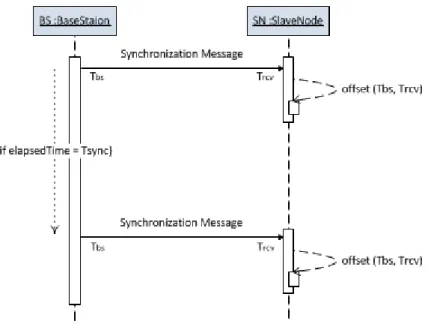
The synchronization phase is based on unidirectional broadcast synchronization. The base station transmits synchronization beacons at regular intervals (Tsync) to its slave nodes. The synchronization message contains a timestamp (Tbs) taken just before the

message’s packet is transmitted on the radio interface (see section 3.5 below). When the node receives the message, it takes the reception timestamp Trcv. Figure 3.1 shows

the message exchange for the synchronization phase. Based on the two timestamps the offset between the node’s local time and the reference time (base station) can be determined by subtracting the two timestamps:

offset = Trcv− Tbs (3.2)

We ignore the propagation delay as we assume a star topology, on a wireless network with communication end points in a body area, i.e. very close to each other. This implies that propagation delay is less than a µs [11]. Based on the change of the clock offset over time, we calculate the clock drift of a node relatively to the base station (ρi→bs ). Using two values of the clock offset at time t1 and t2, a node i can calculate

the clock drift relative to the base station as follow: ρi→bs =

offset_t

2 − offsett1

t2− t1

(3.3) To achieve high precision it is necessary to combine multiple time estimates, based on the change of the clock offset over time, to compensate the clock drift (more details in section 3.4). By knowing Emax and the drift of its clock, each node can determine

(38)

Figure 3.1: Message exchange for the synchronization phase.

when to receive the synchronization beacon, instead of receiving all synchronization beacons sent periodically by the base station.

3.3 Resynchronization

An important parameter that should be determined in order to achieve the required accuracy is the resynchronization interval [29]. In our protocol, the resynchronization interval is fixed and is determinate during the setup phase. It is based on each node’s required accuracy and clock drift.

Since, among all sensor node components, the radio consumes the most significant amount of energy [10], we introduce the ability for the node to decide when resyn-chronize. As nodes receive the beacons they can estimate their clock drift compared with the reference clock. Based on the current offset, the relative clock drift (ρi→bs)

and the Emax, the node decides when to resynchronize (nextSync) so not to exceed Emax:

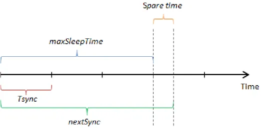
nextSync ≤ Emax − offset ρi→bs

(3.4) nextSync gives an upper bound for the next synchronization interval. Based on Tsync, the node should use the beacon just before nextSync. As an example, if Tsync is 5 seconds, and the node just needs to synchronize in 17 seconds to achieve the required

(39)

CHAPTER 3. ADAPTIVE TIME SYNCHRONIZATION PROTOCOL FOR BANS 39 accuracy, it can stay in the Sleep state during the next two synchronization message (maxSleepTime) and only needs to wake up for the third resynchronization message, changing to the Wait state. This allows the node to save energy while preserving the required time accuracy. As the drift varies, the node may need to wake up more often or may sleep during longer times.

In ideal conditions the node receives correctly the synchronization message. If it misses the synchronization message, due faulty conditions (temporarily unavailable or out of range), the node can request a synchronization message to the base station before compromising the Emax boundary. In section 3.6 we provide a more detailed explanation.

3.4 Drift Compensation

Drift compensation is essential to achieve high precision and to allow nodes to sleep during longer times. Possibly the most used technique is linear regression. Previous works have shown that it can improve the error estimation and the accuracy of clock synchronization [24, 20, 9]. For BANs, this technique has some disadvantages. The clock drift can produce outliers that influence the linear regression [24]. Moreover, the nodes have limited memory and processing power, which limits the number of data points reducing the regression quality [20].

We compensate for clock drift using a weighted moving average filter as in [26]. With this technique we only need to store the last offset average and we use a weight (α) to improve outliers. It improves the clock drift compensation based on the clock offset estimation (offset_avg) along the synchronization process:

offsetvavg = α.offsett+ (1 − α).offsetavgt−1 (3.5)

Initially the value of α is 0.1, i.e. previous samples have more weight that the current sample. We introduce the ability for the node to change α during the synchronization process. External factors, like temperature, can introduce clock drift variations and the current estimation should produce more effect on the clock drift estimation than the previous ones. Moreover, the nodes decide when synchronize and can stay in a sleep state during long periods, which may degrade the quality of the next estimation. The weight of the moving average filter plays an important role here, moving the weight so that the current samples have more effect than the previous ones (increase α), reduces the uncertainty of the drift variation during sleep periods.

(40)

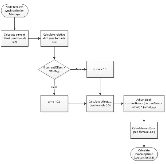
The value of α change based on the current sample and within the interval [0.1, 0.9]. Each time the current sample varies more than 10 ppm (absolute value) relatively to the offset average (offset_avg), the value of α increases by 0,1 until reach the maximum value of 0.9. When the current sample varies less than 10 ppm relatively to the offset_avg, the value of α decreases by 0,1 until reach the minimum value of 0.1. After knowing the current offset and the offset_avg the node can now adjust the clock time relatively to the base station. The clock adjustment process (offset correction and drift compensation) runs each time the node receive a synchronization message. In figure 3.2 we show the node’s flowchart for the clock adjustment process.

(41)

CHAPTER 3. ADAPTIVE TIME SYNCHRONIZATION PROTOCOL FOR BANS 41 As described in section 3.3 each node decides when resynchronize (nextSync). The node uses the synchronization message just before nextSync so not to exceed Emax. The clock adjustment process ends when the node calculates the maximum time that it can sleep.

3.5 Time Stamping

For the accuracy of time synchronization, the time stamping of beacons and received messages is crucial. As we discussed in chapter 2 above, Cox et al. [6] use the SFD of the ZigBee beacon message to distribute the global timestamps. In our protocol, we use the same technique. In figure 3.3 we show how the message time stamping is processed. On the base station side, the timestamp is done deep in the radio layer, immediately after the SFD byte of the synchronization message that is being transmitted. The timestamp is inserted into the MAC frame, known as MAC protocol data units or MPDUs. When the node begins to receive the synchronization message, it takes a timestamp when it receives the SFD. The timestamp is compared later on with the timestamp transmitted by the base station.

Figure 3.3: Time synchronization timestamp. Frame format based on the IEEE 802.15.6 [14].

(42)

This approach allows for highly accurate time synchronization as it eliminates most delay times associated with sending and receiving, namely send, access, reception and receive time. Since the timestamp is inserted when the radio begins the transmission, the transmission time can also be ignored. These times are usually non-deterministic, thus the approach minimizes the delay variability and hence uncertainty. As it is a broadcast scheme without pair-wise message exchange it minimizes energy costs associated with message transmission.

3.6 Message fault tolerance

In ideal conditions the node receives correctly all synchronization messages after the sleep period (wait state). This is not a good assumption. The node can be temporarily unavailable or out of range, and miss the synchronization message. In these situations, instead of waiting for the next synchronization message, that can compromise the Emax boundary imposed by the application requirements, we provide the possibility for the node to request a synchronization message to the base station.

Since nextSync gives an upper bound for the next synchronization interval, the node uses the beacon just before nextSync not to exceed Emax. This allows the node to have a spare time to request a synchronization message to the base station, without exceeding the Emax boundary. Figure 3.4 illustrate this spare time. The node must request a synchronization message before reaching nextSync.

(43)

CHAPTER 3. ADAPTIVE TIME SYNCHRONIZATION PROTOCOL FOR BANS 43 Figure 3.5 illustrates the node’s resynchronization state machine for our synchroniza-tion protocol. The timer2 represent the extra time the node have to request the synchronization message. A further critical problem affecting the proposed message fault tolerance is the case when the node has the maxSleepTime equal to Tsync. Since Tsync is given by the interval needed by the most stringent requirement for accuracy and the worst clock in the system, at least one node may have nextSync equal to Tsync, when its clock drift is at the maximum variation (ρmax). However,

two conditions must occur to affect the reception of the synchronization message: (i) problem in communication and (ii) nextSync equal to Tsync.

Figure 3.5: Slave node resynchronization state machine.

3.7 Efficiency

The efficiency of our protocol depends on the Tsync, at which the base station sends the synchronization messages, and on the application’s requirements. Since nodes do not respond to synchronization messages, the communication cost can be seen as 1 message per Tsync. In the case that the node is faulty (temporarily unavailable or out of range), the communication cost can be seen as 1 + 2n messages per Tsync, where n is the number of nodes that request the synchronization message.

Different applications may require different levels of monitoring and accuracy. These requirements influence the power consumption needed by each node to maintain

(44)

syn-chronized clocks, since they influence the node’s adaptive resynchronization interval. For example, in a fitness monitoring BAN, information about speed, body tempera-ture, oxygen level, and other relevant data can be provided [8]. This information must be correlated in time with certain accuracy. For this scenario, the body temperature sensor can have a maximum error in the order of a few seconds without compromising the application’s objectives. On the other hand, in a firefighting monitoring BAN, firefighter’s information like body temperature, oxygen level, ECG and other relevant data must be correlated in time. If we look again for the body temperature sensor, the maximum time accuracy error must be inferior compared to the first example, since firefighters are exposed to critical environments and a difference in seconds could be vital.

Our protocol adapts to these different levels of monitoring and accuracy. The time synchronization process becomes more efficient in terms of energy cost, without ne-glecting the required accuracy necessary for different applications for BANs. A node can dynamically adapt its synchronization period thus saving energy while keeping accurate.

3.8 Summary and open issues

This chapter presented a time synchronization protocol specific for BANs. The pro-tocol is based on unidirectional broadcast synchronization, where we introduced the ability for the node to decide when to resynchronize. We use a weighted moving average filter to compensate for clock drift. Due to drift variations and long sleep periods, the weight can be adjusted to improve the estimation quality. Our protocol follows the IEEE 802.15 standard guidelines [14].

Currently, we assume that after the base station determines the Tsync, the interval will stay the same during the synchronization process. However, this will not apply to all cases, since new nodes can be introduced, and may need to synchronize at smaller intervals than the initial Tsync. Other issue that needs to be addressed is the fact that the Emax can vary on the same sensor during the synchronization process. For example, if a patient is being monitored and his health condition changes to a critical state, the time accuracy needed may change. To address these issues, nodes should be informed of these changes during the synchronization process. This need to be guarantee in especial cases where critical information is needed. However, since nodes decide when to receive the synchronization messages, the base station does not

(45)

CHAPTER 3. ADAPTIVE TIME SYNCHRONIZATION PROTOCOL FOR BANS 45 know when a node will receive the information. We intend to further investigate the feasibility for the base station, based on bounded drifts, estimate the maximum time that a node will be in a sleep state. Knowing that time the base station can send the new Emax several times to the sensor so that it reaches it. An open solution is the use of wake-up receivers. Wake-up receivers can continuously monitor the channel (with low power consumption), listening for a wake- up signal and wake the sensor node. However it implies different and extra hardware which is a negative point for BAN nodes.

(46)

(47)

Chapter 4 Implementation

This chapter presents the implementation of our time synchronization protocol. It is based on the concepts presented in Chapter 3. The protocol was implemented over Castalia simulator. We improved Castalia with a revised clock where the drift can vary along the simulation time. The implementation source code can be accessed at http://time-synchronization-castalia.googlecode.com.

4.1 Castalia Simulator

The proposed time synchronization protocol was implemented over the Castalia simu-lator [23] for its evaluation. Castalia is a simusimu-lator for Wireless Sensor Networks and Body Area Networks based on the OMNeT++ framework [5]. It has built-in support for modeling wireless channels, node clock drift and the IEEE 802.15.6 standard in BAN MAC.

The OMNeT++ platform is an ”extensible, modular, component-based C++ simu-lation library and framework, primarily for building network simulators”[5]. It is an event-driven simulator where the flow of the simulation is based on the concept of modules and message-passing. Castalia is an extended simulator model enabled by the OMNeT++ framework, and as such it shares the same concept of modules and messages.

Modules and messages

The basic structure of Castalia is composed of nodes, wireless channel and physical 47

(48)

process. These are modules that can communicate through messages. In figure 4.1, we can see the basic module structure of Castalia. The nodes communicate through messages, but not directly. They use the wireless channel module to communicate. There are two types of modules, simple and composite. A simple module can be seen as

Figure 4.1: Castalia module structure from [23].

the execution unit, which receives from other modules, or the module itself, messages to execute a piece of code. A composite module is a module composed by simple modules or other composite modules. Figure 4.2 shows the node composite module. It is composed by simple modules and by a composite module (Communication module). Define Modules

The modules are defined with the use of the OMNeT++ NED language (Network Description). Every module contains a .ned file that defines the basic structure of a module: name, parameters (default values) and interfaces (gates in and gates out). If the module is composite, the .ned file also defines the submodule(s) structure. In the simulation configuration file (omnetpp.ini), the default values defined in the .ned file can be reassigned, enabling a great variety of simulation scenarios. Every module corresponds to a directory in the source code. A directory can have subdirectories if the module is composite. The subdirectories represent the submodules of the composite module. If the module is simple, then there are C++ code files (.cc and .h) that define the actions of the module.

(49)

CHAPTER 4. IMPLEMENTATION 49

Figure 4.2: Node composite module from [23].

4.2 Additions

To properly implement and evaluate the proposed time synchronization protocol, we made changes to some modules of Castalia. Our protocol assumes a clock model with drift variation, i.e. the drift varies over time and the drift and its variability is different for each node. The Castalia simulator provides clock drift for the nodes, but it sets the drift at the beginning of the simulation and assumes a constant drift.

4.2.1 Clock with drift variation

As described in Chapter 2, the clock drift varies over time due to various factors, with the variation of temperature being the main factor. Ageev in [1], shows the influence of the temperature in the clock drift of multiple sensor nodes. He shows that when exposed to a variation of temperature, the clock drift changes substantially. In the evaluation of our protocol, if we assume a constant drift rate, we misrepresent the results. In controlled environments, i.e. environments where external factors do not influence sharply the clock drift, the drift variation is mainly represented by the physical characteristics of the clock (like age), and can be considered constant. But in uncontrolled environments where variation in external factors that influence the clock drift in can occur the same cannot be assumed. We must also point out that in our

(50)

proposal nodes may enter in a sleep state for long periods, and during these periods the drift may vary. If we assume again that the drift has a constant rate, we are assuming a controlled and predictable value, which may not happen in real scenarios. With the last paragraph in mind, we improved Castalia with a revised clock where the drift can vary along the simulation time. The module responsible for the node clock is the TimerService. The clock time can be acquired by calling the public method getClock(). Besides being responsible for the node clock, it is also responsible for defining and managing timers. As show in figure 4.3 , some modules that compose the node, inherit from the TimerService class. This leads to a clock for each module in the same node; the TimerService manages specific timers for each module. For this it keeps track of the offset per TimerService instance and only the drift is defined uniquely for all the modules in the node.

Figure 4.3: Inheritance diagram for TimerService class.

This is not a problem if the clock drift is constant, and set at the beginning of the simulation, but if drift varies we need to adjust all the modules’ clocks during simulation. Moreover, in our proposal we want to correct the clock offset, once again we would need to change all the offsets to have a global time for all the modules that represent the node.

(51)

CHAPTER 4. IMPLEMENTATION 51 ResourceManager module keeps track of some node specific variables, like energy spent, the clock drift and the baseline power consumption [3]. We modify the method getClock() on the TimerService and we use the ResourceManager to maintain the drift variations and the offset corrections. The ResourceManager class is shared between all modules in the node. As shown in figure 4.4, after our modifications, when the method getClock() is called, regardless of the module, all modifications in the clock drift and offset corrections, are retrieved by the ResourceManager and reflected in the clock of each module that inherits from the TimerService class. With these modifications we assure a unique notion of time to all modules that compose the node.

Figure 4.4: Call graph for the getClock() method.

4.2.2 Drift Service Module

We modified the original implementation of Castalia with a revised clock where the clock drift can vary during the simulation, but what values will the drift have and how will it be simulated? To answer that question, we also implemented a specific module that characterizes the clock drift, the DriftService module.

Castalia provides a constant rate clock drift. It is determined from a zero-mean Gaussian random variable and stored in the ResourceManager. At the beginning of the simulation the drift is passed to the TimerService by calling the public method getCPUClockDrift(). With our revised clock implementation, we can change the drift value over time. The DriftService module is responsible to determine new values for the drift and how the drift varies. With this module we enable a variety of simulation scenarios for the clock drift.

(52)

Module definition

We implement the DriftService module as a help structure that can be used optionally (located at /src/helpStrutures in the source code). This way if a module wants to use the DriftService, it must define a list of parameters for the model of the drift variation. In our case, these parameters are located in the synchronization protocol .ned file (/src/node/application/newSyncProtocol/) and are presented below:

double maxDrift = default (0.000100); // 100ppm (parts per million) double minDrift = default (0.000010) // 10ppm (drifts 10us per second)

These are the default maximum and the minimum drift for a given node clock. Each node can have different drift rates.

double maxVariation = default (0.000001); // 1ppm

This is the default maximum variation that a new drift value can have from the last drift value. This value influences how the drift changes, i.e. gradually or drastically. int driftType = default (5); // realistic scenario

The driftType parameter represents one of three drift scenarios. We present these scenarios in Chapter 5. The drift type is represented by an enumerator.

Drift calculation

We use the zero-mean Gaussian function provided by Castalia to calculate new values for the drift, but within the limits [ρmin,ρmax], and with a variation of the drift within

the interval [-ϑmax,ϑmax]. New values for the drift are calculated at regular intervals

(ex: 10 seconds), and this time can be define in the .ned file of the simulation, as also the ϑmax. With this model we can decide how the drift changes over time. The drift

can change gradually or drastically, according the values specified in the .ned file of the simulation.

The new drift value is given by a random value, where ϑmax is the standard deviation

and the current clock drift represents the mean of the Gaussian function. Figure 4.5 shows the call graph for the update drift function. The current clock drift is retrieved by the ResourceManager module. When a new value for the clock drift is calculated it is passed to the ResourceManager, responsible to maintain the drift variations and the offset corrections.

(53)

CHAPTER 4. IMPLEMENTATION 53

Figure 4.5: Call graph for the update drift function.

4.3 Time synchronization module

We implemented our synchronization protocol as an application module. Since our objective regarding the implementation is to make our modifications and new modules available to everyone, the use or not of the time synchronization protocol can be chosen (some applications may not need to use time synchronization) without changing the code.

In figure 4.6 we can easily see the inheritance diagram for the NewSyncProtocol class. The time synchronization protocol interacts directly with the application for the desired time accuracy it needs. The application declares its time requirements (Emax ), and other parameters like the drift variation boundaries of its clock (given by the hardware manufacturer).

Figure 4.6: Inheritance diagram for the NewSyncProtocol class.

The Time Synchronization module defines a set of parameters that can be specified.

These parameters are located in the newSyncProtocol.ned file (src/node/application/newSyncProtocol/), and are presented below:

bool canSleep = default (true); // to enable/disable the sleep functionality bool isBS = default (false); // to identify the Base Station

Adaptive Time Synchronization Protocol for BANS

Paulo Fernando Pereira Vilares

Adaptive Time Synchronization

Protocol for BANs

Departamento de Ciˆ

encia de Computadores

Faculdade de Ciˆ

encias da Universidade do Porto

Adaptive Time Synchronization

Protocol for BANs

Abstract

Contents

List of Tables

List of Figures

Chapter 1

Introduction

1.1

Body Area Networks

1.2

Time Synchronization

1.3

Time Synchronization in Body Area Networks

1.4

Contributions

1.5

Dissertation Structure

Chapter 2

Time Synchronization

2.1

Clocks

2.2

Sources of time synchronization errors

2.3

Synchronization approach

2.4

Communication schemes

2.5

Time synchronization for Body Area Networks

2.5.1

Network topology

2.5.2

Applications requirements

2.5.3

Heterogeneous sensors

2.5.4

Energy efficiency

2.6

Traditional time synchronization protocols

2.7

Wireless sensor network synchronization

pro-tocols

2.8

WSN vs. BAN

Chapter 3

Adaptive Time Synchronization

Protocol for BANs

3.1

Why adaptive?

3.2

Synchronization scheme

3.3

Resynchronization

3.4

Drift Compensation

3.5

Time Stamping

3.6

Message fault tolerance

3.7

Efficiency

3.8

Summary and open issues

Chapter 4

Implementation

4.1

Castalia Simulator

4.2

Additions

4.2.1

Clock with drift variation