1
FORTNIGHTLY CHANGES IN WATER TRANSPORT DIRECTION ACROSS THE MOUTH OF A NARROW ESTUARY
Erwan Garel, Óscar Ferreira
CIMA (Centre for Marine and Environmental Research)
Universidade do Algarve ,Edifício 7, Campus de Gambelas, 8005 - 139 Faro, Portugal Phone: 00 351 289 800 900 Ext. 7899
Fax: 00 351 289 800 069
Corresponding author: E. Garel (egarel@ualg.pt)
2
Abstract
This research investigates the dynamics of the axial tidal flow and residual circulation at the lower Guadiana Estuary, south Portugal, a narrow mesotidal estuary with low freshwater inputs. Current data were collected near the deepest part of the channel for 21 months and across the channel during two (spring and neap) tidal cycles. Results indicate that at the deep channel depth-averaged currents are stronger and longer during the ebb at spring and during the flood at neap, resulting in opposite water transport directions at a fortnightly time scale. The net water transport across the entire channel is up-estuary at spring and down-estuary at neap, i.e. opposite to the one at the deep channel. At spring tide, when the estuary is considered to be well-mixed, the observed pattern of circulation (outflow in the deep channel, inflow over the shoals) results from the combination of the Stokes transport and compensating return flow, which varies laterally with the bathymetry. At neap tide (in particular for those of lowest amplitude each month), inflows at the deep channel are consistently associated with the development of gravitational circulation. Comparisons with previous studies suggest that the baroclinic pressure gradient (rather than internal tidal asymmetries) is the main driver of the residual water transport. Our observations also indicate that the flushing out of the water accumulated up-estuary (at spring) may also produce strong unidirectional barotropic outflow across the entire channel around neap tide.
Keywords
3
Introduction
Quantification of the patterns of water circulation in estuaries is fundamental for studying ecological processes and for sustainably managing these systems. In tide-dominated systems, tidal currents may induce large fluxes of nutrients and of contaminants over short (diurnal or semi-diurnal) time scales (e.g. Dale and Prego 2003; Gardner and Kjerfve 2006). At subtidal time scales, residual (tidally-averaged) currents govern the net exchange of material with the adjacent coastal area, and are therefore of great importance for the health of estuarine ecosystems (e.g. Whiting and Childers 1989; Gao et al. 2008).
The along-channel (axial) residual circulation in estuaries is controlled mainly by the relative importance of gravitational stability and turbulent mixing, which originates from the interaction of freshwater inflow, tides and wind (Mantovanelli et al. 2004; Uncles and Stephens 1990). The control by gravitational stability and turbulent mixing produces two major flow components, the tidally-induced and density-induced flows, which compete against each other to determine residual flows (Jay and Smith 1990; Li et al. 1998). Tidally-driven residual flows are produced by the difference in phase between the horizontal (current) and vertical (elevation) tide, by tidal non-linearities produced by horizontal gradients in tidal velocities (divergence and lateral shear), and also by variations in the mean sea level at the entrance of the estuary caused by such phenomena as remote winds (Li and O´Donnell 1997; Valle-Levinson et al. 2009; Winant and Gutiérrez de Velasco 2003). Density-driven residual currents are produced by baroclinic circulation, which is induced by the longitudinal density gradient (Pritchard 1956; Pritchard 1960), and by intra-tidal asymmetries in both turbulent mixing and stratification (Jay and Musiak 1996; Scully and Friedrichs 2007). Both mechanisms (baroclinic pressure gradient and intra-tidal asymmetries) produce the typical estuarine (or gravitational) circulation of partially-stratified estuaries, characterised by a tidally-averaged exchange flow which is oriented up-estuary near the bed and down-estuary near the surface (Stacey et al. 2001). Lateral bathymetric variations greatly influence the intensity and direction of residual currents, both tidally- and density-induced (de Jonge 1992; Kjerfve and Proehl 1979; Valle-Levinson et al. 2009; Waterhouse and Valle-Levinson 2010). In particular, observations and analytical models have indicated that the direction of axial residual currents along the deepest channel is often opposite to that over the adjacent shoals (Li and O´Donnell 1997; Li and O'Donnell 2005; Scully and Friedrichs 2007; Valle-Levinson et al. 2003; Winant 2008; Wong 1994).
The above depicts a large variability in the water circulation dynamics at the mouth of estuaries. Observations are fundamental for model validation and to understand the factors controlling water transport in distinct settings. For example, the direction of axial residual flows might be assumed to be constant across the channel of narrow (less than 1 km in width) estuaries. The present paper shows that this is not the case, based on observations near the mouth of a mesotidal, narrow estuary with low river inflow. Current data were collected at a fixed station for a period of 21 months, and across the channel during two tidal cycles, at spring and at neap. The objectives are (i) to describe the axial tidal and subtidal water circulation and its lateral variability, and (ii) to compare the patterns of variation of the residual water transport with those predicted by analytical models. The paper is organized as follows. Background information to the study site is presented in the next section, followed by details about the data acquisition and processing. The results section includes general tidal information from long-term observations, and describes the water circulation patterns at tidal and subtidal time scales. The patterns of the residual transport, and its driving mechanisms, are then discussed and compared with previous studies.
4
Study Area
The Guadiana Estuary extends for 80 km in a north-south direction at the Portugal/Spain border (Fig. 1). The estuarine channel is narrow (max. 700 m wide near the mouth), and connects the Guadiana River directly to the open littoral zone (the Gulf of Cadiz). Typically, the transverse morphology consists of a single deep channel bordered by shoaling areas (Fig. 1). The maximum depth of the channel (with respect to mean water level) is generally less than 10 m, with a mean depth of about 5 m from the mouth to km 50 upstream (Lobo et al. 2004).
fig
Figure 1. Location of the measurements along the transect (solid line, Tr) and at the fixed station (dot, XR) at the lower Guadiana Estuary. Urbanized areas are in black. The dashed lines mark the boundary between the deep channel and adjacent shoaling areas. The bathymetric cross-section along the transect line (Tr) is shown on the top right corner.
The tidal signal in the area is regular, semidiurnal and mesotidal, with mean tidal ranges of 1.28 m at neap and 2.56 m at spring, and a maximum of 3.44 m (Instituto Hidrografico 1990). Scarce data suggest a ~2 h lag between maximum surface amplitude and peak currents near the mouth (Silva et al. 2003).
The river discharge into the estuary is extremely low throughout the year, generally less than 20 m3 s-1, due to strong flow regulation by upstream dams. Under these conditions, the lower estuary is considered as well-mixed at spring tide, with unidirectional seaward vertical velocity profiles attributed to the barotropic tide (Garel et al. 2009a). At neap, the lower estuary is partially-stratified, and characterised by the typical two-layer flow of the estuarine
5
circulation (Garel et al. 2009a). The alternating establishment and breakdown of the two-layer residual flow with neap and spring tides, respectively, denotes strong variations in the relative significance of tidally- and density-driven currents on a fortnightly time scale.
Data and Methods
Measurements
Current measurements were collected with an Acoustic Doppler Profiler (ADP) equipped with internal pressure and temperature sensors (Sontek Argonaut XR 750 kHz; XR hereafter), which is part of an autonomous system for the long-term monitoring of currents and of water quality (including surface temperature; for details, see Garel and Ferreira 2011; Garel et al. 2009b). The XR was bottom-mounted in the lower estuary, near the deepest part of the channel, at ~ 10 m water depth at high tide (Fig. 1). Data were recorded continuously from 18 March 2008 to 15 December 2009, with some large data gaps in May-June 2008 and April-June 2009 due to technical problems. During the study period, the river discharge was lower than 20 m3 s-1, except in February 2009 when the discharge increased moderately (up to 200 m3 s-1) for a few days. Data were sampled and averaged at five minute intervals, every 0.8 m along the water column. The 1st measuring cell was 1.8 m from the bed, due to the blanking distance and the height of the mooring structure.
Currents were also measured along a transect line (Tr) perpendicular to the estuarine channel at about 100 m upstream from the XR, with a hull-mounted ADP (Sontek 1.5 MHz; Fig. 1). At this location, the deepest part of the channel (referred to hereafter as the deep channel) leads up to an embankment at the Portuguese margin. Eastward of the deep channel, the bed shoals in a regular fashion towards the intertidal areas of the Spanish margin. A cross-channel profile was measured every 30 min for 13 h (i.e. 26 profiles) at both spring and neap tides (17 September 2008, 3.01 m tidal range; 21 October 2008, 1.59 m tidal range). The velocity of the boat was about 1 m s-1, weather conditions were fair and the river discharge was less than 13 m3 s-1 during both surveys. The ADP was used in bottom-tracking mode, and velocity profiles were obtained as ensembles averaged over 5 s, in cells of 0.5 m-thick. The blanking distance was 0.5 m, and the instrument head was at 0.38 cm and 0.22 cm below the water surface at spring and neap tide, respectively.
Data processing
Fixed station
For the (bottom-mounted) XR data, quality tests were performed based on instrument tilting, standard deviation of the records and signal noise ratio of the beams (with threshold values based on the manufacturer’s recommendations). The bin located immediately below the water surface was discarded to avoid any potential boundary interference affecting velocity measurements. Data were interpolated using a constant 15 min interval throughout the study period. Pressure records were converted into water depths based on daily atmospheric pressure from a meteorological station located at Tavira (20 km at west of the Guadiana mouth). The north and east components of the current velocities were rotated along the axis of maximum variance (11.5ºE of north) to an along- and across-channel coordinate system; only the along-channel (or axial) velocity component, u (m s-1, positive up-estuary) is considered in the present paper. The depth-averaged velocity U (m s-1) was computed internally by the XR as the integration of the velocities measured along the water column (the end of the measurement volume close to the surface is adjusted automatically based on the
6
pressure records). It was checked that similar depth-averaged values were obtained based on the integration of the records along the validated bins. Residual values were derived from low pass-filtering using a Butterworth filter of 40 h cut-off period. To compute residual velocities along the water column, the height from the bed, z (m), was normalised to the water depth, h (m), with z/h=0 at the bed and 1 at the water surface.
The residual depth-averaged fluxes of water were separated into their various components: non-tidal drift, Stokes transport and mass transport (Uncles et al. 1985). The residual current (i.e. non-tidal drift, V1) contains a downstream directed residual flow component which compensates the (upstream) Stokes transport (V2). Stokes transport results from the variation with time of the estuarine channel cross-section during the passage of the (partially progressive) tidal wave. V2 was estimated based on the fluctuating parts of water depth (h
~
) and current velocity ( 1
~ V ), with: hV h V2 ~~1 / (1) and h h h~ and 1 1 ~ V U V (2)
where diamond brackets denote a residual. The residual mass transport (or mass flux) velocity (V3) is defined as (Zimmerman 1979):
2 1 3 V V
V (3)
The residual mass transport velocity results from linear processes (wind, river discharge and gravitational circulation) and tidal non-linearities (Jiang and Feng 2011). V3 is appropriate for describing the mean water circulation in tidal environments because it is conserved at a section of an estuary, whereas V1 is not (Wei et al. 2004).
Tidal constituents of the sea surface elevation and depth-averaged axial velocity were computed based on data from 20 June 2008 to 29 March 2009, i.e. the longest time series with no significant data gaps, using the T_TIDE software package (Pawlowicz et al. 2002). Principal component analysis (PCA) was applied to the velocities recorded from 1 July 2008 to 1 January 2009. This study followed the method of Stacey et al. (2001), who applied PCA to separate the vertical structure of the barotropic boundary layer from the two- layer exchange flow of the estuarine circulation in a tidally-dominated system. Non-interpolated velocities (rather than interpolated values at normalised depth) were used, so the points always have the same elevation with respect to the bed. However, because PCA requires a rectangular matrix, only four cells were considered in order to limit extrapolation or interpolation in the cells above the tidally fluctuating surface. Some older data recorded in deeper water (i.e. in 12 cells, at minimum) at the entrance of the Guadiana Estuary were used to verify that four cells were sufficient to resolve the spatial structure of the exchange flow. Transect line data
The threshold of the signal-to-noise ratio of the hull-mounted ADP records was set to 3 dB to remove invalid data below the ambient noise level. Axial velocities were derived from the projection of the east and north velocity components along the axis defined by the channel orientation (10ºW of north). To compute residuals, velocity records were gridded at a resolution of 50 m (cross-channel distance) by 0.1 (normalised depth). The tidal and residual
7
signals were then separated through a least squares fit to semi-diurnal (M2) harmonic (Lwiza et al. 1991).
The components (V1, V2 and V3) of the residual depth-averaged fluxes of water were obtained similarly than from the XR data (equations 1 to 3, where tidally-averaged values are the mean over the tidal period of the data interpolated at a one-minute interval; Kjerfve 1975). For these calculations (only), the transect line was divided into five sections (A to E) of 90 m instead of using the gridded data, in order to optimise the averaging of ADP ensembles while accounting for lateral variability in the bathymetry. Sections A and B correspond to the deep channel, Sections C and D to the central estuarine channel, and section E to the shallowest part of the channel (Fig. 1). The boat-derived transects generally extended further eastward than section E (up to 550 m) but these data were not considered for the computation of the residual water flux components, due to very shallow water depths at low tide. For each section, U was computed as the integral of the depth-averaged velocities of each ensemble within the considered section:
d hu y z dydz h d U 0 0 ) , ( 1 1 (4)
where y (m) is the distance along the section and d is the total length of the section (90 m). RESULTS
Tidal information
The main tidal constituents of the pressure and axial velocities at the XR location are reported in Table 1. The semi-diurnal band (all components) represented 82% of the total water level amplitude and 81% of the current amplitude. By comparison, the contribution of the diurnal band components to the water level and current amplitudes was relatively small (9% and 6 %, respectively), although much larger than the contribution of the quarter diurnal (M4)
component (1.8% and 2% of the water level and current amplitude, respectively). The large elevation amplitude ratio (M2/M4) indicates that the tidal wave is weakly distorted at the
mouth (Speer and Aubrey 1985).
The difference in phase between elevation and current at the semi-diurnal frequency was 57º. Likewise, the coherence squared from a cross-spectral analysis between pressure and axial current amplitudes yielded a phase of 58º at the semi-diurnal frequency. This means that the tide at the entrance of the estuary is partially progressive, with peak currents preceding maximum tidal stage by 2 h, in agreement with previous estimates (Silva et al. 2003).
Table 1. Tidal amplitude, phase and phase difference (95% confidence interval) of the largest diurnal (K1
),semi-diurnal (M2) and quarter-diurnal (M4) frequencies for the XR (based on records from 20/06/2008 to
29/03/2009), as calculated from sea surface elevation (m) and axial depth-averaged velocity (U ) using T_TIDE (Pawlowicz et al. 2002).
Sea surface elevation U
Amplitude (m) Phase (º) Amplitude (m s
-1
)
Phase (º) Phase difference (º)
K1 0.065 54 0.034 344 -70
M2 0.983 62 0.807 5 57
8
Tidal flow
Observations at the fixed station
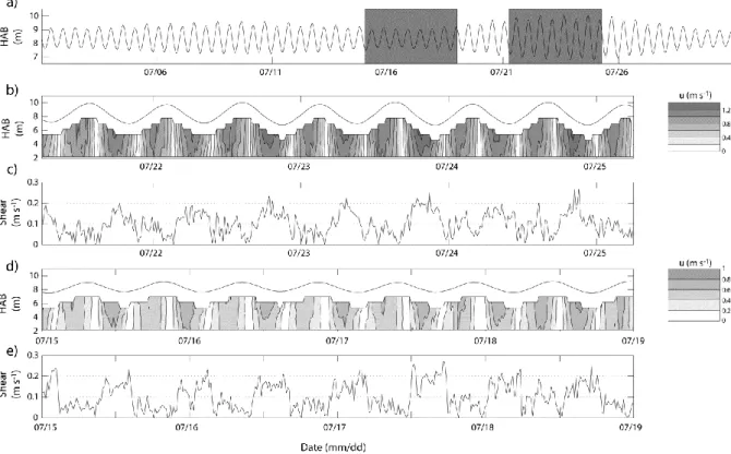
The typical variations of axial currents with depth and over a tidal month are shown in Figure 2. Maximum currents were observed near the surface during both spring and neap tides (Fig. 2b, d). This behaviour reflects the major role of friction over the vertical structure of the tidal flow. However, friction alone is unable to explain the markedly greater vertical shear during ebb than during flood, which is observed for similar (ebb and flood) velocities (Fig. 2c, e). Especially during neap tides, the maximum vertical shear on the ebb was as large as that during spring tide (and often stronger) despite much lower velocities. In addition, the shear at neaps presented an unsteady behaviour characterized by two sharp peaks, one close to maximum velocities and the other (generally the strongest peak) at slack ebb.
Figure 2. a) Height above bed (HAB, m) at the XR location; the grey areas indicate data subsets for spring (b, c) and neap (d, e) tides; b) vertical structure of the currents (u, m s-1) at spring tide (see scale); c) vertical shear at spring tide; d) vertical structure of the axial currents at neap tide (same scale as in b); e) vertical shear at neap tide.
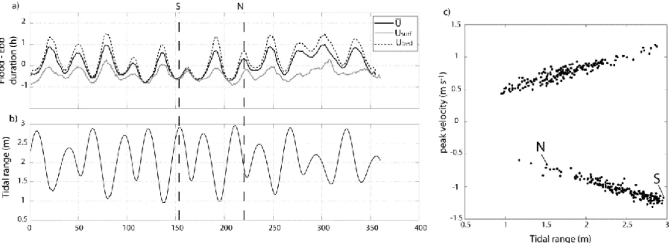
Tidal asymmetries were analysed in terms of peak velocity and tidal phase (ebb and flood) duration from 1 July 2008 to 1 January 2009 (Fig. 3). Considering depth-averaged velocities, floods were longer around neaps whilst ebbs were longer around springs; the largest asymmetries were generally at neaps, up to ~1 h (Fig. 3a, b). In comparison, the duration of the ebb and flood was enhanced near the surface and near the bed, respectively, especially around neaps. The maximum (depth-averaged) velocities were generally ebb-directed at spring tides, and flood-directed at neap tides (Fig. 3c); yet, this behaviour was not verified during the neap tidal cycle survey (ebb-directed peak velocities; see N on Fig. 3c). The transition between ebb- and flood-directed peak currents corresponded roughly to the tidal range of 2 m. It is important to note that at neaps, generally, surface velocities were larger on the ebb in relation to the strong shear of the flow (see Fig. 2), but the maximum depth-averaged and near-bed velocities were observed on the flood.
9
Figure 3. Tidal asymmetries at the XR location based on records from 1 July 2008 to 1 January 2009: a) difference in duration (h) between the flood phase and the ebb phase of each tidal cycle, considering the depth-averaged velocities (U , solid black line), the near-surface flow (Usurf, solid grey line) and the near-bed flow
(Ubed, dashed black line); the data were smoothed using a 10-point moving average; b) tidal amplitude (m); c)
peak velocity (m s-1, flood positive, ebb negative) against tidal amplitude (m) for the tidal cycles during the period considered. ). S: tidal cycle survey at spring tide; N: tidal cycle survey at neap tide.
Observations along the transect line
Axial currents across the channel were related to bed friction, with peak velocities over the deep channel and near the surface (Fig 4a, b, e, f). Around slack water, a significant lateral shear was observed because current reversal occurred first over the shoals and subsequently at the deep channel due to the relatively larger flow momentum over the deepest areas (Fig. 4c, d, g). However, at slack ebb of the neap tide the flow was sheared vertically (rather than laterally) with flood- and ebb-oriented currents near the bed and near the surface, respectively (Fig. 4h).
Subtidal flow
Mass transport velocity and tidal range
The components of the residual depth-averaged currents exhibited consistent patterns of variation with the tidal range at the fixed station (Fig. 5a, b, c). Residual velocities (V1) were generally weakly upstream at neaps, and strongly downstream at springs. The downstream residuals at springs included a significant seaward-directed component which compensates the relatively strong upstream Stokes transport (V2, up to ~0.05 m s-1). At neaps, the Stokes transport was not significant due to the reduced amplitude of the tidal elevations and currents (the water discharges near high and low water are similar). These modulations of V1 and V2 at a fortnightly time scale produced a marked variability in the intensity and direction of the residual mass water transport velocity (V3, Fig. 5c). Around springs, V3 was down-estuary and relatively weak (up to ~0.05 m s-1), except for some large outflows due to the advection of freshwater from upstream dams in April 2008 (probably, although no river discharge data were available) and in February 2009. Residual near-bed and near-surface currents indicate that the vertical structure of the flow was unidirectional during these periods of down-estuary transport (Fig. 5d). This pattern contrasts with the strong (up to ~0.1 m s-1) up-estuary pulses of V3 at neap tides (Fig. 5c), which were systematically associated with the typical two-layer flow of the estuarine circulation (Fig. 5d). These pulses were modulated at a monthly time scale, the greatest ones occurring during the weakest neap tides (Fig. 5a, c).
10
A significant (p < 0.01) inverse Pearson’s linear correlation was calculated between V3 and tidal range, with a coefficient of correlation R of -0.58 (Fig. 6). The water transport direction reversed for tidal ranges of approximately 2 m.
Figure 4. Axial velocity (m s-1) across the channel (x-axis, m) and along the water depth (y-axis, m) at spring tide (left) and at neap tide (right). The graphs are based on transects performed at peak flood currents (a, b), slack flood (c, d), peak ebb currents (e, f) and slack ebb (g, h). The graphs showing peak velocities (a, b, e, f) have the same grey scale (darker: faster currents; lighter: slower currents) and a contour interval of 0.2 m s-1. For the graphs around slack water (c, d, g, h), the contour interval is 0.1 m s-1 and the light (dark) grey corresponds to up-estuary (down-estuary) oriented velocities. Keys: HW: High Water; LW: Low Water; W: Western margin; E: Eastern margin.
Cross-channel variability
At spring tide, the non-tidal drift (V1) was directed down-estuary at all sections across the channel, and included a relatively large compensatory flow as indicated by the significant Stokes transport (V2) values, about 0.05-0.06 m s-1 (Fig. 7a). As a result, the mass flux velocity (V3) was up-estuary across the entire channel, except in the deep channel (Section A, down-estuary) in agreement with the results at the XR location (XR in Fig. 7a; see also S line in Fig. 5). V3 was largest in the middle of the channel (Sections C and D). The average mass transport across the entire channel was oriented upstream (Channel in Fig. 7a).
11
Figure 5. Results at the fixed station (XR, 18 March 2008 to 15 December 2009): a) tidal range (m); b) non-tidal drift (V1, solid line, m s-1) and Stokes transport (V2, dashed line, m s-1); c) mass transport velocity (V3, m s -1); d) Low-passed near-bed (dashed line) and near-surface (solid line) axial velocities (m s-1). The dashed
vertical lines extending through all diagrams indicate the dates of the tidal cycle surveys across the channel at spring (S) and neap (N) tides. Negative (positive) values refer to downstream (upstream).
At neap tide, the mass flux velocity was downstream at all sections including in the deep channel, also in agreement with the XR results (Fig 7b; see also the N line in Fig. 5). In fact, V3 was equivalent at each section to the one at spring tide, but with the additional contribution of a strong (0.05 to 0.0 8 m s-1) downstream component. The average mass transport across the entire channel was downstream (Channel in Fig. 7b), i.e. opposite to the transport direction at spring tide.
Figure 6. Residual mass water transport velocity (V3, m s-1) against tidal ranges (m) at the fixed station. For
clarity, only the crests and troughs of the V3 signal were considered. Negative (positive) values refer to
12
The residual vertical velocity profiles were unidirectional (oriented down-estuary) across the entire channel at spring and neap tides (Fig. 8), again in agreement with the XR results (see N and S lines in Fig. 5d). A strong lateral shear was generally observed, with the weakest residuals in the centre of the channel. At neap tide, however, a strong vertical shear was also observed over the thalweg (Fig. 8b).
Figure 7. Components of the depth-averaged residual flow (in cm s-1) at (a) spring and (b) neap tide. Non-tidal drift (V1, circle), Stokes transport (V2, asterisk) and mass flux velocities (V3, diamond) from sections A to E
across the channel (white area), for the entire channel (mean of the sections, light grey area) and at the XR location (dark grey area).
Figure 8. Residual axial velocity (cm s-1) across the channel (x-axis, m) and along the normalised water depth (z/h, m) at spring tide (left) and neap tide (right). The contour interval is 3 cm s-1. White area: no data (due to insufficient sampling points at low tide).
Barotropic and baroclinic flows
Spring-neap variability
When PCA is used on multiple-depth current data in a tidally dominated system, the first component (PC1) represents the tidal barotropic currents (Stacey et al. 2001). The second component (PC2) can then be analyzed for any evidence of density-driven currents. In agreement, the analysis of the XR data resulted in a PC1 that was the barotropic boundary layer, and a PC2 that was a sheared, exchange flow profile. The dataset was strongly
13
dominated by PC1, which defined 99.78% of the variance. PC2 defined almost all (0.20%) the remaining variance. Similar results were obtained at the St Lawrence Estuary, a macro-tidal estuary with periodic stratification (Simons et al. 2010).
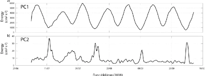
The energy (square of the speed) of the near-bed currents due to PC1 and PC2 were low-pass filtered to remove tidal variations (Fig. 9). PC1 shows the expected barotropic fluctuations in energy between spring (up to 6000 cm2 s-2) and neap (around 1000 cm2 s-2). The energy of the PC2 component was relatively low at spring (~5 cm2 s-2) but was characterised by pulses (increasing by a factor of ~6) during the neap tides of lowest amplitude.
Figure 9. Spring-neap variability in energy (cm2 s-2) of the near-bed PC1 (a) and PC2 (b) current components.
Tidal cycle variability
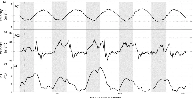
The dynamics of the pulses of PC2 at neap were examined at the tidal time scale based on five consecutive tidal cycles in July 2008 (Fig. 10a, b). The difference between the temperatures at the surface and near the bottom is also displayed as a qualitative surrogate of vertical density differences, and thus of stratification (Fig. 10c). This approach is possible because riverine water is distinctly warmer than seawater in summer.
The PC1 component shows the typical variations of the barotropic tide, and is used to distinguish between the ebb (grey areas) flood phases (Fig. 10a). The PC2 component displays a strong ebb-flood variability, which is characterised in the first order by positive values during the ebb (> 0.1 m s-1) and negative values fluctuating between zero and -0.25 m s-1 during the flood. A striking similarity between these PC2 variations and the water column stratification (top-bottom difference in temperature) is observed (Fig. 10 b, c). In a general way, the PC2 and stratification increased together during the ebb and tended to zero during the flood. In detail, the positive values of PC2 correspond to two distinct pulses which are clearly associated with peaks in the stratification: the first pulse is associated with the maximum barotropic (PC1) ebb velocities; the second pulse is observed on the early flood and is followed by a negative spike that is quickly dampened out with increasing barotropic flood currents. The negative PC2 spikes (reverse of the estuarine circulation) indicate that the water column remained stratified and created a sheared profile after the ebb as well (see Cheng et al. 2010).
14
Figure 10. Tidal cycle variability in the axial velocity (m s-1) of PC1 (a) and of PC2 (b) components; c) top-bottom difference in temperature (δt, ºC). The grey areas denote ebb tide, as defined based on the PC1 component near the bed.
DISCUSSION
Spring-neap variability of residual flows
A central result of this study is the change in direction of the residual water transport on a fortnightly time scale at the deep channel of the Guadiana Estuary. For tidal amplitudes less than ~2 m, gravitational circulation is associated with strong pulses of water landward; for higher tidal ranges, the water transport is seaward with unidirectional residual velocity profiles (Figs. 5, 6 and 9). These observations strongly suggest that the residual flows near the mouth are predominantly barotropic when the estuary is well-mixed (spring tide) and baroclinic when it is partially-stratified (neap tide). In fact, there is a striking similarity in the variations of V3 and of the PC2 energy at neap (compare Figs. 5c and 9b), which confirms that the upstream residual mass transport at neap results from monthly pulses in the strength of the gravitational circulation. Typically, in estuaries characterised by density-driven flow, stronger exchanges develop at neaps than at springs (Haas 1977; Nunes and Lennon 1987). In contrast, the strongest exchange occurs at springs in estuaries with tidally-driven flows (e.g. Valle-Levinson et al. 2009). In mesotidal and macrotidal estuaries with freshwater inputs, these opposite modulations compete to determine the net water transport; they are responsible for spring-neap variations in water transport intensity (e.g. the James River Estuary; Li et al. 1998), but more rarely in direction as observed in this study.
The residual inflows (outflows) at the deep channel of the Guadiana Estuary result from the enhancement of both the duration and peak velocity of flood (ebb) currents (Fig. 3). Neap-spring variations in the pattern of tidal asymmetries generally result from the modulation of stratification (enhanced at neaps) and friction (enhanced at springs) (Uncles 2002). At the study site, the reinforcement of the stratification at neaps is well-illustrated by the vertical shear at that time, which is as large as at springs despite weaker currents (Fig. 2c, e). However, the mechanisms which determine the direction (up- or down-estuary) of residual flows at the Guadiana Estuary are not established. The dynamics of the observed (barotropic
15
and baroclinic) residual flows are discussed in the sections below, based on comparisons with predictions from analytical models.
Barotropic residual flow
Classification of the estuarine system
Recent analytical models have indicated that the direction of the tidally-induced residual circulation depends on the phase difference between surface elevation and tidal velocities near the open end of the tidal basin (Winant 2008; Winant and Gutiérrez de Velasco 2003). This phase difference determines if the tidal wave is standing (current and elevation out of phase) or not. The progressive component of the tide depends on the length of the estuary and on the relative importance of bottom friction (Li and O'Donnell 2005). Hence, tidal estuaries are conveniently distinguished according to either their length or their frictional effects. Li and O’Donnell (2005) computed the ratio (r) between the geometric length of the channel and the quarter of the tidal wavelength to separate long (r > 0.6-0.7, progressive tidal wave) and short (r < 0.6-0.7, standing tidal wave) estuaries. Alternatively, Winant (2008) classified tidal channels, based on a friction factor (F) that represents the influence of friction on flow dynamics at a tidal inlet, as either strong (F=1), moderate (F=0.5) or weak (F=0.1). In his analytical model, Winant considered the problem in 3D through the inclusion of Earth rotation effects and depth-dependent flow. For narrow systems where Coriolis effects can be neglected, including the Guadiana Estuary, the solutions of Li and O’Donnell (vertically integrated flows) and Winant (transport stream function) are equivalent (Valle-Levinson et al. 2009).
Following Li and O’Donnell (2005), the length ratio r is about 1 at the Guadiana Estuary,
which means that residuals induced by the phase difference between tidal elevation and tidal current are close to maximum values. In addition, Winant’s friction factor F is moderate at the XR location (F=0.4 and 0.8 for the semidiurnal M2 tide and a vertical eddy viscosity of 0.001 and 0.005 m2 s-1, respectively). This is in agreement with the relatively small value of the M4 overtide (Table 1) and the lack of ebb- or flood-dominance (i.e. ebb or flood faster but shorter, typically found in strongly frictional systems) (Aubrey and Speer 1985; Fig. 3). Hence, it seems reasonable to compare (in the next section) our results at the well-mixed narrow Guadiana Estuary (i.e. at spring tide) with the analytical solutions for long estuaries characterized by moderate friction.
Residuals and Stokes transport
In long estuaries with moderate to strong friction, the progressive component of the tidal wave is responsible for an upstream Stokes transport which is larger over the shoals than in the deep channel (Li and O´Donnell 1997). The Stokes flux produces a water level set-up towards the estuary head. This set-up induces a seaward residual pressure gradient that creates a barotropic return flow oriented down-estuary, which is larger in the thalweg than over the shoals. The combination of Stokes transport and return flow produces an outward and an inward residual flow in the thalweg and over the shoals, respectively (Li and O'Donnell 2005; Winant 2008).
This pattern of residual circulation has been described in well-mixed and weakly-stratified estuaries with widths of kilometric order or more (e.g. Cáceres et al. 2003; Kjerfve and Proehl 1979; Li et al. 1998). Near the mouth of the narrow Guadiana Estuary, the mass transport was also down-estuary in the deep channel and up-estuary over the shoals at spring
16
tide (Figs. 5 and 7), and resulted in an upstream transport across the entire channel (see “Channel” in Fig. 7a). This circulation pattern corresponds to the one resulting from the Stokes transport (and return flow) mechanism. In order to illustrate the set-up that is induced upstream by the Stokes transport, water level time-series were obtained from a hydrographic station located in the upper estuary (Alcoutim, 40 km from the mouth) during two periods: (1) April 2003 to March 2004, and (2) March to May 2008 (the only observations coinciding with the XR measurements). The low-pass filtered 2003-2004 time-series (40 hr cut-off period) showed successive rising and lowering of the water level around spring and neap tides, respectively, of about 30 cm in amplitude (Fig. 11a). The peaks (October and November 2003; April 2004) correspond to episodic water releases from dams. Spectral analysis confirmed the predominance of the fortnightly tidal frequency in the signal (not shown). Between March and May 2009, a similar fortnightly tide was observed in the upper estuary (Fig. 11b). Water level variations at the XR during the same period were comparatively much lower in amplitude, and did not oscillate at a fortnightly frequency. This dataset confirms the net transport of water up-estuary around spring tide, which is induced by a significant Stokes transport.
Figure 11. Water level variations (m), (a) from April 2003 to April 2004 at Alcoutim (40 km upstream from the mouth) and, (b) from 15 March 2008 to 15 May 2008 at the XR location (dark grey) and at Alcoutim (light grey). Residuals are shown as thick black lines.
Barotropic outflow across the entire channel
It is important to note that the fortnightly oscillations in water level in the upper estuary are produced because the downstream return flow rarely compensates exactly for the Stokes transport at the tidal time scale. Depending on the barotropic forcing, water level either increases or decreases upstream, and the return flow is respectively weaker or larger than the Stokes transport. During the tidal cycle survey at neap, gravitational circulation was not observed (N line in Fig. 5d and fig. 8b). Moreover, maximum (depth-averaged) velocities were observed during the ebb, as opposed to the asymmetry which is generally observed at neaps (flood faster; see Fig. 3c). Thus, it seems that tidally-driven circulation dominated during this particular tidal cycle, following the mechanism described above for spring tides. In addition, the downstream residual mass transport velocity was much greater than at spring (despite relatively lower Stokes transport), due to the addition of a strong downstream component (Fig. 7). Although more data are needed to confirm this point, it is likely that this downstream component corresponds to the flushing down-estuary of (excess) water accumulated upstream.
17 Internal tidal asymmetries
Our observations strongly support the significance of the wave propagation and mean pressure gradient in creating the residual axial flow pattern at spring tide near the mouth of the Guadiana Estuary. However, density gradients were not considered so far. Recent numerical simulations, analytical models and direct observations have suggested that internal tidal asymmetries in stratification may be predominant in the creation of residual currents, even in well-mixed environments (Becherer et al. 2011; Burchard et al. 2008; Burchard et al. 2011; Winant 2010). Previous studies at the lower Guadiana Estuary have indicated that a weak straining of the density field may occur during the ebb at spring tide (Garel et al. 2009a). In the present study, the longer duration of ebbs near the surface than near the bed also points to potential stratification periods at spring (Fig. 3a). Tidal straining also explains why the vertical shear is stronger during ebbs than during floods, despite similar velocities (Fig. 2b, c).
The residual pattern of variation produced by internal tidal asymmetries is described as outflow at the deep channel and inflow over the shoal (Scully and Friedrichs 2007), i.e. similar to our observations at springs. Thus, internal tidal asymmetries may add up to the Stokes transport mechanism to produce the observed residual flow pattern. However, the normalized overtide current amplitude (the ratio of the M4 constituents from current and
elevation divided by the ratio of the M2 constituents from current and elevation) is 1 (see
Table 1), indicating that non-linearities driven by internal tidal asymmetries are generally absent at the mouth (Jay and Musiak 1996). The contribution of internal tidal asymmetries to residual currents is likely to be negligible in most cases and especially at spring tide; however, it could be of significance episodically, in particular when estuarine circulation develops, as discussed in the next section.
Gravitational circulation
Mechanisms creating residuals
The creation of estuarine circulation is generally attributed to two mechanisms: (1) the baroclinic circulation which is driven by the longitudinal density gradient (Hansen and Rattray 1965); and (2) the barotropic exchange flow, which is created by asymmetries in turbulent mixing and stratification between the ebb and the flood (Cheng et al. 2011; Simpson et al. 1990). Numerical solutions have indicated that the flow driven by internal tidal asymmetries may be as important as the density-driven flow for estuarine circulation in narrow, partly mixed estuaries (Cheng et al. 2011). Determining whether the residual-creating estuarine circulation is due to the baroclinic pressure gradient or to barotropic forcing is not unequivocally possible on the basis of the dataset presented in this study. On the one hand, the gravitational circulation is rather persistent throughout the neap tidal cycles, including during the flood (indicated by negative PC2 values), as expected from a constant background circulation produced by a baroclinic pressure gradient (Fig. 10b). Furthermore, the exchange flow is large (null) when the stratification is well-developed (weakly-developed) (Fig. 10), as also expected from a baroclinic mechanism (e.g. Nunes Vaz et al. 1989). On the other hand, the largest pulses of PC2 occur at a time (around slack ebb) that is consistent with a water column undergoing strain-induced periodic stratification (Simpson et al. 2005). Accordingly, the strongest shear of the velocity profiles at neap tide is observed around slack ebb (Fig. 2e), as expected from reduced vertical mixing and enhanced stratification (e.g. Uncles 2002). In fact, a two-layer flow was observed at that time over the deep channel (Fig. 4h). It seems
18
therefore that both mechanisms (barotropic and baroclinic) act to create the estuarine circulation at the Guadiana Estuary.
Several studies have indicated that in estuaries with significant lateral variations in density gradients, the baroclinic circulation favours inflows in channels, and favours outflows over the shoals where stratification is reduced by mixing and tidal non-linearities are enhanced (Lerczak and Geyer 2004; Li et al. 1998; Valle-Levinson et al. 2003; Wong 1994). Conversely, an opposite pattern (inflow over the shoals, outflow at the deep channel) is observed in estuaries with lateral variations in internal tidal asymmetries, because tidal straining reduces mixing and enhances the duration of the ebb in the deep channel (Scully and Friedrichs 2007). In the present study, gravitational circulation was not developed during the neap tidal cycle survey, precluding the study of lateral variations in residual water transport. Nevertheless, residual directions at neap at the deep channel (inflows) are in agreement with the pattern described for flows driven by a baroclinic pressure gradient (Fig. 5). This observation suggests that the baroclinic pressure gradient is the dominant mechanism in creating the residual inflow at the partially-stratified Guadiana Estuary.
CONCLUSIONS
This study has presented observations of the axial tidal and subtidal flows at the lower mesotidal and narrow Guadiana Estuary, based on current measurements at a fixed station for 21 months and across the channel during two (spring and neap) tidal cycles. The objectives were to explicitly define the intensity and direction of residual flows, and to identify the main drivers of the net water circulation.
The results indicate that tidal asymmetry at the deep channel is characterised by longer and stronger (depth-averaged) currents during the ebb at spring tide and during the flood at neap tide. These asymmetries produce a residual water transport which is modulated at a fortnightly time scale (inflows at neap, outflows at spring). The switch in the net transport directions at the deep channel occurs for tidal amplitudes of ~2 m, the average tidal range in the area, which was also the approximate tidal range below which estuarine circulation developed. The residual transport across the entire channel is up-estuary at spring and down-estuary at neap, i.e. opposite to the one at the deep channel.
At spring tides, observations indicate that even very narrow estuaries such as the Guadiana Estuary (700 m-wide at most) may display significant lateral variations in the residual axial flows. The pattern of residual circulation (outflow in the deep channel, inflow over the shoals) was consistent with previous observations and analytical solutions for other tidally-dominated systems with progressive tidal wave components. This pattern is determined by the combination of the Stokes transport and compensating return flow, which varies laterally with the bathymetry.
At neap tides (especially those of lowest amplitude each month), inflows at the deep channel result from pulses of estuarine circulation. These pulses vary at the tidal time scale, being stronger during the ebb. A contentious issue in the literature concerns whether gravitational circulation is driven by the baroclinic pressure gradient or by internal tidal asymmetries in mixing and stratification (e.g. Li and Zhong 2009). Our results suggest that both processes contribute to the residual-creating exchange flow at narrow, partially-stratified systems such as the Guadiana Estuary at neap tide. However, comparisons with previous studies indicate that ultimately it is the baroclinic pressure gradient which predominantly drives the residual inflow at the estuarine thalweg.
19
In addition, this study reports a neap tidal cycle during which the tidally-induced residual water transport was stronger than at spring tide, presumably as a result of the flushing out of the excess of water upstream. In this case, a strong barotropic flow is able to produce unidirectional outflows across the entire channel.
This study also exemplifies how non-tidal drift may occur in the opposite direction to mass transport in estuaries where the standing tidal wave includes a significant progressive component. At these sites, the mass transport velocity should be considered for computations of advective transport and suspended material flux.
Acknowledgements
Centre for Science (Centro Ciência Viva) from Tavira is acknowledged for the atmospheric pressure data. Thanks are extended to A. Pacheco for assistance in collecting data. E. Garel benefited from FCT (Fundação para a Ciência e Tecnologia, Portuguese National Board of Scientific Research) grants SFRH/BPD/34475/2005. The bottom-mounted current-meter is part of a monitoring station (Simpatico system) that was acquired through a FCT grant for the re-equipment of scientific institutions (Reeq/484/MAR/2005). We are also grateful to two anonymous reviewers who have contributed significantly to improve the quality of the original manuscript.
References
Aubrey, D.G. and P.E. Speer. 1985. A study of non-linear tidal propagation in shallow inlet/estuarine systems Part I: Observations. Estuarine, Coastal and Shelf Science 21: 185-205.
Becherer, J., G. Burchard, G Floser, V. Mohrholz and L. Umlauf. 2011. Evidence of tidal straining in well-mixed channel flow from micro-structure observations. Geophysical Research Letters 38: L17611.
Burchard, H., G. Flöser, J.V. Staneva, T.H. Badewien and R. Riethmüller. 2008. Impact of Density Gradients on Net Sediment Transport into the Wadden Sea. Journal of Physical Oceanography 38: 566-587.
Burchard, H., R.D. Hetland, E. Schulz and H.M. Schuttelaars. 2011. Drivers of Residual Estuarine Circulation in Tidally Energetic Estuaries: Straight and Irrotational Channels with Parabolic Cross Section. Journal of Physical Oceanography 41: 548-570.
Cáceres, M., A. Valle-Levinson and L. Atkinson. 2003. Observations of cross-channel structure of flow in an energetic tidal channel. Journal of Geophysical Research 108 3114.
Cheng, P., A. Valle-Levinson and H.E. de Swart. 2010. Residual Currents Induced by Asymmetric Tidal Mixing in Weakly Stratified Narrow Estuaries. Journal of Physical Oceanography 40: 2135-2147.
Cheng, P., A. Valle-Levinson and H.E. de Swart. 2011. A numerical study of residual circulation induced by asymmetric tidal mixing in tidally dominated estuaries. Journal of Geophysical Research 116: C01017.
Dale, A. W. and R. Prego. 2003. Tidal and seasonal nutrient dynamics and budget of the Chupa Estuary, White Sea (Russia). Estuarine, Coastal and Shelf Science 56: 377-389.
de Jonge, V.N. 1992. Tidal flow and residual flow in the Ems estuary. Estuarine, Coastal and Shelf Science 34: 1-22.
20
Gao, L., D.-J. Li and P.-X. Ding. 2008. Nutrient budgets averaged over tidal cycles off the Changjiang (Yangtze River) Estuary. Estuarine, Coastal and Shelf Science 77: 331-336.
Gardner, L. R. and B. Kjerfve. 2006. Tidal fluxes of nutrients and suspended sediments at the North Inlet–Winyah Bay National Estuarine Research Reserve. Estuarine, Coastal and Shelf Science 70: 682-692.
Garel, E. and Ó. Ferreira. 2011. Monitoring estuaries using non-permanent stations: practical aspects and data examples. Ocean Dynamics 61: 891-902.
Garel, E., L. Pinto, A. Santos and Ó. Ferreira. 2009a. Tidal and river discharge forcing upon water and sediment circulation at a rock-bound estuary (Guadiana estuary, Portugal). Estuarine, Coastal and Shelf Science 84: 269-281.
Garel, E., S. Nunes, J.M. Neto, R. Fernandes., R. Neves, J.C. Marques and Ó. Ferreira. 2009b. The autonomous Simpatico system for real-time continuous water-quality and current velocity monitoring: examples of application in three Portuguese estuaries. Geo-Marine Letters 29: 331-341.
Haas, L.W. 1977. The effect of the spring-neap tidal cycle on the vertical salinity structure of the James, York and Rappahannock Rivers, Virginia, USA. Estuarine and Coastal Marine Science 5: 485-496.
Hansen, D.V. and M.J. Rattray. 1965. Gravitational circulation in straits and estuaries. Journal of Marine Research 23: 104-122.
Instituto Hidrografico, 1990. Roteiro da Costa de Portugal. Instituto Hidrografico, Lisboa, 504 pp.
Jay, D.A. and J.D. Musiak. 1996. Internal tide asymmetry in channel flows: Origins and consequences. In: C.B. Pattiaratchi (Editor), Mixing in estuaries and coastal seas, coastal and estuarine studies. American Geophysical Union, Washington DC, pp. 211-249.
Jay, D.A. and J.D. Smith. 1990. Residual Circulation in Shallow Estuaries 2. Weakly Stratified and Partially Mixed, Narrow Estuaries. Journal of Geophysical Research 95: 733-748.
Jiang, W. and S. Feng. 2011. Analytical solution for the tidally induced Lagrangian residual current in a narrow bay. Ocean Dynamics 61: 543:558.
Kjerfve, B. 1975. Velocity averaging in estuaries characterized by a large tidal range to depth ratio. Estuarine and Coastal Marine Science 3: 311-323.
Kjerfve, B. and J.A. Proehl. 1979. Velocity variability in a cross-section of a well-mixed estuary. Journal of Marine Research 37: 409-418.
Lerczak, J.A. and R.W. Geyer. 2004. Modeling the Lateral Circulation in Straight, Stratified Estuaries. Journal of Physical Oceanography 34: 1410-1428.
Li, C. and J. O´Donnell. 1997. Tidally driven residual circulation in shallow estuaries with lateral depth variation. Journal of Geophysical Research 102: 27915-27929.
Li, C., A. Valle-Levinson, K.C. Wong and K.M.M. Lwiza. 1998. Separating baroclinic flow from tidally induced flow in estuaries. Journal of Geophysical Research 103: 10405-10417.
Li, C.Y. and J. O'Donnell. 2005. The effect of channel length on the residual circulation in tidally dominated channels. Journal of Physical Oceanography 35: 1826-1840.
Li, M. and L. Zhong. 2009. Flood-ebb and spring-neap variations of mixing, stratification and circulation in Chesapeake Bay. Continental Shelf Research 29: 4-14.
Lobo, J., F. Plaza, R. Gonzáles, J. Dias, V. Kapsimalis, I. Mendes and V.D.d. Rio. 2004. Estimations of bedload sediment transport in the Guadiana Estuary (SW Iberian Peninsula) during low river discharge periods. Journal of Coastal Research12-26.
21
Lwiza, K.M.M., D.G. Bowers and J.H. Simpson. 1991. Residual and tidal flow at a tidal mixing front in the North Sea. Continental Shelf Research 11: 1379-1395.
Mantovanelli, A., E. Marone, E.T. Silva, L.F. Lautert, M.S. Klingenfuss, V.P.J. Prata, M.A. Noernberg, B.A. Knoppers and R.J. Angulo. 2004. Combined tidal velocity and duration asymmetries as a determinant of water transport and residual flow in Paranaguá Bay estuary. Estuarine, Coastal and Shelf Science 59: 523-537.
Nunes, R.A. and G.W. Lennon. 1987. Episodic stratification and gravity currents in a marine environment of modulated turbulence. Journal of Geophysical Research 92: 5465-5480.
Nunes Vaz, R.A., G.W. Lennon and J.R. de Silva Samarasinghe. 1989. The negative role of turbulence in estuarine mass transport. Estuarine, Coastal and Shelf Science 28: 361-377.
Pawlowicz, R., B. Beardsley and S. Lentz. 2002. Classical tidal harmonic analysis including error estimates in MATLAB using T_TIDE. Computers & Geosciences 28: 929-937. Pritchard, D.W. 1956. The dynamic structure of a coastal plain estuary. Journal of Marine
Research 15: 33-42.
Pritchard, D.W., 1960. Lectures on estuarine oceanography, J. Hopkins University, 154 pp. Scully, M.E. and C.T. Friedrichs. 2007. The Importance of Tidal and Lateral Asymmetries in
Stratification to Residual Circulation in Partially Mixed Estuaries. Journal of Physical Oceanography 37: 1496-1511.
Silva, A.J.d., S. Lino, A.I. Santos and A. Oliveira, 2003. Near bottom sediment dynamics in the Guadiana Estuary. In: Thalassas (Editor), 4th Symposium on the Iberian Atlantic Margin, pp. 180-182.
Simons, R.D., S.G. Monismith, F.J. Saucier, L.E. Johnson and G. Winkler. 2010. Modelling stratification and baroclinic flow in the estuarine transition zone of the St. Lawrence estuary. Atmosphere-Ocean 48: 132 - 146.
Simpson, J.H., J. Brown, J. Matthews and G. Allen. 1990. Tidal straining, density currents, and stirring in the control of estuarine stratification. Estuaries 13: 125-132.
Simpson, J.H., E. Williams, L.H. Brasseur and J.M. Brubaker. 2005. The impact of tidal straining on the cycle of turbulence in a partially stratified estuary. Continental Shelf Research 25: 51-64.
Speer, P.E. and D.G. Aubrey. 1985. A study of non-linear tidal propagation in shallow inlet/estuarine systems Part II: Theory. Estuarine, Coastal and Shelf Science 21: 207-224.
Stacey, M.T., J.R. Burau and S.G. Monismith. 2001. Creation of residual flows in a partially stratified estuary. Journal of Geophysical Research 106: 17013-17043.
Uncles, R.J. 2002. Estuarine Physical Processes Research: Some Recent Studies and Progress. Estuarine, Coastal and Shelf Science 55: 829-856.
Uncles, R.J., R.C.A. Elliott and S.A. Weston. 1985. Observed fluxes of water, salt and suspended sediment in a partly mixed estuary. Estuarine, Coastal and Shelf Science 20: 147-167.
Uncles, R.J. and J.A. Stephens. 1990. The structure of vertical current profiles in a macrotidal, partly-mixed estuary. Estuaries 13: 349-361.
Valle-Levinson, A., C. Reyes and R. Sanay. 2003. Effects of Bathymetry, Friction, and Rotation on Estuary–Ocean Exchange. Journal of Physical Oceanography 33: 2375-2393.
Valle-Levinson, A., G.G.d. Velasco, A. Trasviña, A.J. Souza, R. Durazo and A.J. Mehta. 2009. Residual Exchange Flows in Subtropical Estuaries. Estuaries and Coasts 32: 54-67.
22
Waterhouse, A. and A. Valle-Levinson. 2010. Transverse structure of subtidal flow in a weakly stratified subtropical tidal inlet. Continental Shelf Research 30: 281-292. Wei, H., D. Hainbucher, T. Pohlmann, S. Feng and J. Suendermann. 2004. Tidal-induced
Lagrangian and Eulerian mean circulation in the Bohai Sea. Journal of Marine Systems 44: 141-151.
Whiting, G. J. and D. L. Childers. 1989. Subtidal advective water flux as a potentially important nutrient input to southeastern U.S.A. Saltmarsh estuaries. Estuarine, Coastal and Shelf Science 28: 417-431.
Winant, C.D. 2008. Three dimensional residual tidal circulation in an elongated, rotating, basin. Journal of Physical Oceanography 38: 1278-1295.
Winant, C.D. 2010. Two-layer circulation in a frictional, rotating basin. Journal of Physical Oceanography 40: 1390-1404.
Winant, C.D. and G. Gutiérrez de Velasco. 2003. Tidal dynamics and residual circulation in a well-mixed inverse estuary. Journal of Physical Oceanography 33: 1365-1379.
Wong, K.C. 1994. On the nature of transverse variability in a coastal plain estuary. Journal of Geophysical Research 99: 14209-14222.
Zimmerman, J. 1979. On the Euler-Lagrange transformation and the Stokes’ drift in the presence of oscillatory and residual currents. Deep-Sea Research 26A: 505-520.